Mathematics 9709/55 — May/June 2025
Cambridge AS Level · Probability & Statistics 1 · worked solutions for every part, with the mark scheme
Topics Discrete Random Variables · The Normal Distribution · Probability · Representation of Data · Permutations and Combinations
Two fair 6-sided dice with faces labelled 1, 2, 3, 4, 5, 6 are thrown. The two scores are noted. The random variable is defined as follows.
● If the two scores are equal,
● If the scores are not equal, is the larger score minus the smaller score
Approach
List all equally likely ordered pairs from two dice. For each possible value of , count how many pairs give that score difference and divide by to obtain probabilities.
Working
There are equally likely ordered outcomes , where is the score on the first die and the score on the second.
- : the two scores are equal; outcomes.
- : pairs with difference , such as and ; outcomes.
- : outcomes.
- : outcomes.
- : outcomes.
- : outcomes.
So the probability distribution table is:
| 0 | 1 | 2 | 3 | 4 | 5 | |
|---|---|---|---|---|---|---|
Check: .
Answer
The probability distribution of is given by the completed table above.
P(X=0)=1/6, P(X=1)=5/18, P(X=2)=2/9, P(X=3)=1/6, P(X=4)=1/9, P(X=5)=1/18
Walkthrough
We need a probability distribution table for , where is the absolute difference between two dice scores (with when they are equal). Each die has 6 faces, so there are equally likely ordered outcomes; the order matters because the dice are separate objects. For each possible difference , count the ordered pairs. For example, can come from , giving outcomes. After counting all values, divide each count by and simplify. This gives the table, and the probabilities should sum to .
Key Takeaways
A random variable assigns a numerical value to each outcome of a random experiment. To build a probability distribution, count outcomes for each value, divide by the total number of outcomes, and present the values with their probabilities. The probabilities in a distribution table must always sum to .
Common Mistakes
- Counting un-ordered pairs instead of ordered pairs, so missing half of the outcomes such as treating and as the same.
- Forgetting that equal scores give , not difference from different dice.
- Using or another total instead of outcomes.
- Rounding each probability and then finding that they do not add exactly to ; work with fractions to keep the table exact.
Things to Be Careful About
Use ordered pairs throughout. The maximum possible difference is when one die shows and the other shows . Always include . Check the sum of probabilities is exactly before moving on.
Approach
Use the expectation formula and the variance formula .
Working
Next find :
Then:
Answer
E(X) = 35/18, Var(X) = 665/324
Walkthrough
From the table, every probability is a fraction over (or its simplified form). To find , multiply each value of by its probability and add the products: . This gives , which simplifies to . For variance, the formula is easiest. Compute by multiplying each by its probability, giving . Then subtract the square of the mean: .
Key Takeaways
Expectation is the weighted mean of the random variable, and variance measures the spread around that mean. The formula avoids calculating deviations individually and is central to discrete random variables.
Common Mistakes
- Calculating as ; these are different quantities.
- Forgetting to subtract when finding variance.
- Arithmetic slips when squaring or combining denominators; use a common denominator.
- Not identifying which answer is and which is ; the mark scheme requires the final values to be clearly identified.
Things to Be Careful About
Keep exact fractions throughout, since decimal rounding may lose marks unless the question asks for an approximation. The variance may be written as . Make sure to use the table’s probabilities, including the contribution (which is zero in both sums but must not be forgotten conceptually).
The heights of trees in a certain forest are classified as tall, medium or small. The heights can be modelled by a normal distribution with mean and standard deviation . Trees with a height of less than are classified as small.
For 150 randomly chosen trees from this forest, how many would you expect to be classified as small?
Approach
Let be the height of a randomly chosen tree. The heights are modelled by
A tree is small if . Standardise using the -score formula, find the lower-tail probability, then multiply by the number of trees.
Working
Standardise the cutoff height :
Therefore
Using the symmetry of the normal distribution and the standard normal table, , so
The expected number of small trees out of 150 is
Answer
17 or 18 trees expected (expected value 17.265)
Walkthrough
First write down the model: a randomly chosen tree height is normally distributed with mean m and standard deviation m. The phrase 'less than m' selects the lower tail of this distribution. To use the standard normal table, convert into a -score: subtract the mean and divide by the standard deviation, giving .
The standard normal table normally gives probabilities of the form for positive . Because is negative, use symmetry: is the same as . From the table, , so the required lower-tail probability is .
Finally, the expected number of small trees among 150 is the probability multiplied by 150: . Since this is a count of trees, give an integer conclusion such as 17 or 18 expected trees.
Key Takeaways
This question tests the standardisation step , using the symmetry of the normal curve to evaluate a negative -score, and interpreting a probability as a long-run proportion to find an expected frequency.
Common Mistakes
- Forgetting to subtract from 1 when the required tail is below a negative -score and the table gives .
- Reversing the order in the standardisation formula, e.g. using instead of .
- Stopping at the probability 0.115 and not multiplying by 150.
- Giving a non-integer decimal as the expected 'number of trees' without recognising that an integer count is required; here the raw expected value is 17.265, so 17 or 18 is accepted.
Things to Be Careful About
- The standard deviation is m, not ; use , not the variance, in the denominator.
- Do not apply a continuity correction: the heights are modelled directly as normal, so no continuity correction is needed.
- The symbol denotes the cumulative standard normal probability; make sure the final probability is sensible (less than 0.5, since m is below the mean m).
Trees from this forest are classified as tall if their height is at least . 25% of the trees are classified as tall.
Find the value of .
Approach
Let be the height that separates the tallest 25% from the rest. Since 25% of trees are tall, the upper tail above has probability 0.25, so the lower tail below has probability 0.75. Find the standard normal -value corresponding to cumulative probability 0.75, then solve the standardisation equation for .
Working
We need
so
From the standard normal table, the value with cumulative probability 0.75 is
Standardising :
Solve for :
Therefore, to one decimal place,
Answer
h = 23.4 m
Walkthrough
The key is to translate the percentage into a probability statement. If 25% of trees are tall, then the upper tail above height has probability 0.25. The normal table usually gives lower-tail probabilities, so convert to the lower tail: .
Now find the -score that has cumulative probability 0.75. From standard normal tables, this is (the 75th percentile of the standard normal distribution). The height is above the mean because the 75th percentile of a normal distribution lies above the centre, so is positive.
Standardise using : set . Multiplying by 5 gives , so m, or 23.4 m to one decimal place.
Key Takeaways
This question tests converting a percentile (or tail percentage) into a -score and reversing the standardisation formula to find the original value. It also reinforces that the upper-tail probability 0.25 corresponds to cumulative probability 0.75 in the lower tail.
Common Mistakes
- Treating 0.25 or 0.75 as if it were the -score instead of using the table to find the -score with cumulative probability 0.75.
- Using a negative -score; since is in the upper 25%, is above the mean and the -score must be positive.
- Using the variance or in the denominator instead of the standard deviation 5.
- Incorrectly setting ; remember the upper tail given is 0.25, so the lower tail is 0.75.
Things to Be Careful About
- The phrase 'tall if height is at least ' means the upper tail is because the distribution is continuous, so equality makes no difference.
- The critical value 0.674 is a -value, not a probability. Do not confuse values such as 0.5987, 0.7734 or 0.326 with the needed -score.
- Round the final height to the required accuracy; here 23.37 m rounds to 23.4 m.
In a certain large school, on average, two pupils in five have music lessons.
A random sample of 80 pupils from this school is chosen.
Use an approximation to find the probability that fewer than 27 pupils have music lessons.
Approach
Let be the number of pupils in the sample who have music lessons. The exact distribution is binomial, . Since is large, approximate by a normal distribution with the same mean and variance, and use a continuity correction before standardising.
Working
The probability that a pupil has music lessons is
For :
so
Use the normal approximation . The event 'fewer than 27' becomes after the continuity correction.
Standardise:
Therefore
Answer
0.105
Walkthrough
We are told that on average two pupils in five have music lessons, so the probability that a randomly chosen pupil has music lessons is .
For a sample of 80 pupils, the number with music lessons has a binomial distribution. Because 80 is large, we may use a normal approximation. The first step is to match the normal distribution to the binomial by using its mean and variance:
The binomial variable takes only whole-number values, but the normal variable is continuous. The event 'fewer than 27' includes . To translate this discrete event onto the continuous scale, we treat it as values up to . This is the continuity correction.
Next we standardise:
The required probability is the area under the standard normal curve to the left of . Since the normal curve is symmetric, this equals . From normal tables, , so:
Key Takeaways
- The binomial distribution with large can be approximated by a normal distribution.
- The approximate normal distribution uses the same mean and variance as the binomial.
- A continuity correction is essential when a discrete count is approximated by a continuous curve.
- Standardisation converts the normal approximation into the standard normal distribution so tables can be used.
Common Mistakes
- Forgetting the continuity correction and using directly in the standardisation.
- Using the variance in the denominator instead of the standard deviation .
- Taking the area to the right of instead of the left, or failing to subtract from .
- Using the exact binomial calculation instead of the normal approximation requested by the question.
Things to Be Careful About
- 'Fewer than 27' excludes 27, so the corrected boundary is , not .
- Use in the standardisation formula.
- The final probability should be less than ; if it is not, check the sign of the -value or which tail has been found.
- The mark scheme accepts a final answer in the range , so values such as are expected after rounding.
A random sample of 10 pupils from this school is now chosen.
Find the probability that no more than 2 pupils have music lessons.
Approach
Let be the number of pupils in the sample of 10 who have music lessons. Since the sample is from a large school, it is reasonable to treat the selections as independent with probability ; hence . 'No more than 2' means , so add the three binomial probabilities.
Working
For :
Thus
Evaluating each term:
Answer
0.167
Walkthrough
Again is the probability that a randomly chosen pupil has music lessons. The sample size is 10, so let be the number of pupils in the sample with music lessons; then .
'No more than 2' means , or . These are mutually exclusive, so we add the three probabilities.
For a binomial distribution:
So:
Evaluate each term:
Rounding to 3 significant figures gives .
Key Takeaways
- This is an exact binomial probability question, not a normal approximation.
- The probability of no more than 2 is found by adding the probabilities of 0, 1 and 2.
- The terms are mutually exclusive, so addition is valid.
Common Mistakes
- Using the normal approximation for a sample of size 10; is too small.
- Forgetting the binomial coefficient .
- Evaluating only the term for and not including and .
- Confusing 'no more than 2' with 'fewer than 2', which would be or only.
Things to Be Careful About
- and must both be used correctly, with the powers swapped in each term.
- Use the complement method only if you are careful to subtract all cases from 3 to 10.
- The mark scheme accepts , so quote at least 3 significant figures.
Students applying to Drydale College take an entrance test. A student is either accepted or rejected or required to take another test with probabilities 0.3, 0.2 and 0.5 respectively. When a student takes a second test the outcomes and probabilities are exactly the same as for the first test. A student who has to take a third test is accepted with probability 0.25 and rejected with probability 0.75.
Approach
Draw a tree diagram with three stages representing the test outcomes. The first two stages have three branches each (Accepted, Rejected, Test again), and the final stage has two branches (Accepted, Rejected).
Working
The first branch splits into:
- Accepted (A) with probability
- Rejected (R) with probability
- Test again (T) with probability
From the first 'Test again' node, the branches split again with the same probabilities:
- Accepted (A) with probability
- Rejected (R) with probability
- Test again (T) with probability
From the second 'Test again' node, the student takes a third test with different probabilities:
- Accepted (A) with probability
- Rejected (R) with probability
Answer
The tree diagram is constructed as described above.
Tree diagram as shown in diagram-1
Walkthrough
The question describes a sequential testing process with three possible stages. We model this using a tree diagram where each node represents a decision point or test outcome.
First, we draw the initial branch for the first test. The student can be Accepted (A) with probability , Rejected (R) with probability , or required to take another test (T) with probability . These three outcomes are mutually exclusive and exhaustive, so their probabilities sum to .
If the student is not rejected, they proceed to a second test. The problem states the outcomes and probabilities are exactly the same as the first test. So from the first 'T' node, we draw three branches: A (), R (), and T ().
If the student is still not rejected, they proceed to a third test. The probabilities for this third test are different: Accepted () and Rejected (). Since there are only two outcomes, these sum to , and we stop here.
Key Takeaways
- Tree diagrams are ideal for representing sequential probability problems with multiple stages.
- The probabilities along any single path from the root to a leaf are multiplied to find the probability of that specific sequence of events.
- Branches from a single node must sum to .
Common Mistakes
- Forgetting that the third test has different probabilities ( and ) than the first two tests.
- Adding extra branches or missing the end of the tree when a student is accepted or rejected.
Things to Be Careful About
- Ensure all branches from each node sum to exactly .
- Label all branches clearly with both the outcome name and the probability to avoid confusion in later parts.
Find the probability that a randomly chosen student who applies to Drydale College is accepted.
Approach
A student can be accepted on the first test, the second test, or the third test. These are mutually exclusive events. Calculate the probability of each path and sum them using the addition law of probability.
Working
The paths to acceptance are:
- Accepted on the first test:
- Test again, then accepted on the second test:
- Test again twice, then accepted on the third test:
Total probability of acceptance:
This can also be written as .
Answer
0.5125
Walkthrough
To find the total probability that a student is accepted, we must consider all the distinct ways this can happen. Looking at the tree diagram, there are three terminal nodes where the outcome is 'Accepted':
- The student is accepted immediately on the first test. The probability is simply the branch probability: .
- The student is not accepted on the first test (must take another test, probability ), and then is accepted on the second test (probability ). By the multiplication law, this path has probability .
- The student is not accepted on the first two tests (probabilities ), and then is accepted on the third test (probability ). This path has probability .
Since these three events cannot happen at the same time, they are mutually exclusive. We add their probabilities:
Key Takeaways
- The addition law of probability states that the probability of a union of mutually exclusive events is the sum of their individual probabilities.
- The multiplication law is used to find the probability of a sequence of dependent events (a path down the tree).
Common Mistakes
- Forgetting one of the paths to acceptance (e.g., only considering the first test).
- Adding probabilities along a single path instead of multiplying them.
Things to Be Careful About
- Ensure you have identified ALL paths that lead to the desired outcome. In this case, acceptance can happen at any of the three test stages.
Find the probability that a randomly chosen student who applies to Drydale College takes at least two tests given that the student is accepted.
Approach
Use the conditional probability formula . Here, is 'accepted' and is 'takes at least two tests'. We need to find the probability of taking at least two tests AND being accepted, then divide by the total probability of being accepted.
Working
Let be the event 'accepted' and be the event 'takes at least two tests'.
The event corresponds to the paths where the student takes at least two tests and is eventually accepted. These are:
- Test again, then accepted:
- Test again twice, then accepted:
So, .
From part (b), we know .
Applying the conditional probability formula:
Simplifying the fraction:
As a decimal, this is approximately or to 3 significant figures.
Answer
17/41
Walkthrough
We are asked for the probability that a student takes at least two tests, given that they are accepted. This is a classic conditional probability problem.
The condition is that the student is accepted. So our sample space is restricted to only the outcomes where the student is accepted. The total probability of being accepted is , which we calculated in part (b).
Now, within this restricted sample space, we want to find the probability that the student took at least two tests. The paths where a student is accepted AND takes at least two tests are:
- First test: Test again (), Second test: Accepted (). Probability = .
- First test: Test again (), Second test: Test again (), Third test: Accepted (). Probability = .
The sum of these probabilities is .
Using the formula :
Key Takeaways
- Conditional probability restricts the sample space to the given condition.
- The formula is fundamental for solving these problems.
- Always clearly define what events and represent before applying the formula.
Common Mistakes
- Forgetting to divide by the probability of the condition (part b's answer).
- Including the path 'Accepted on first test' in the numerator, which does not involve taking at least two tests.
Things to Be Careful About
- Ensure you correctly identify the intersection . 'Takes at least two tests' means the student did not get accepted or rejected on the first test.
Three friends apply to Drydale College.
Find the probability that all three are rejected.
Approach
First, find the probability that a single student is rejected. Then, since the three friends apply independently, use the multiplication law to find the probability that all three are rejected.
Working
The probability that a student is accepted is (from part b).
The probability that a student is rejected is the complement:
Alternatively, summing the rejection paths:
Since the three friends apply independently, the probability that all three are rejected is:
Calculating this:
Rounding to 3 significant figures, we get .
Answer
0.116
Walkthrough
The problem asks for the probability that all three friends are rejected. First, we need the probability that any single student is rejected.
From part (b), we know the probability of acceptance is . Since a student is either accepted or rejected (the 'test again' paths eventually lead to acceptance or rejection), the probability of rejection is simply the complement:
We can verify this by summing the probabilities of all paths ending in 'Rejected':
- Rejected on first test:
- Rejected on second test:
- Rejected on third test:
- Total:
The three friends apply independently, meaning the outcome for one does not affect the others. Therefore, we multiply the probability of rejection for each friend:
Key Takeaways
- The complement rule is a quick way to find the probability of rejection once acceptance is known.
- Independence allows us to multiply probabilities for multiple events occurring together.
Common Mistakes
- Forgetting that 'test again' paths eventually end in rejection or acceptance, so .
- Not cubing the probability for the three independent friends.
Things to Be Careful About
- Ensure the final answer is given to an appropriate number of significant figures (3 SF is standard unless specified otherwise). rounds to .
The Smarts and the Teasers are two quiz teams that each contain 11 members. Both complete a puzzle and the following table gives the times taken, in minutes, by the members of each team.
| Smarts | 38 | 30 | 13 | 29 | 18 | 22 | 28 | 18 | 11 | 9 | 41 |
|---|---|---|---|---|---|---|---|---|---|---|---|
| Teasers | 39 | 37 | 18 | 36 | 25 | 25 | 32 | 21 | 15 | 12 | 39 |
Represent this information in a back-to-back stem-and-leaf diagram with Smarts on the left-hand side.
Approach
Sort the data for both teams in ascending order. Place the stems (tens digits) in the centre column. Write the leaves (units digits) for Smarts on the left in descending order from the stem, and for Teasers on the right in ascending order. Include a key.
Working
The sorted data for Smarts is: .
The sorted data for Teasers is: .
Constructing the back-to-back stem-and-leaf diagram:
Key: means minutes for Smarts and minutes for Teasers.
Answer
Diagram constructed as shown in the working.
Diagram constructed as shown in the working.
Walkthrough
First, sort both sets of data in ascending order to make it easier to extract the stems (tens digits) and leaves (units digits). For Smarts, the sorted times are . For Teasers, they are .
Next, set up the stem-and-leaf diagram with the stems in the centre column. The stems range from to . For the left-hand side (Smarts), write the leaves in descending order away from the stem so that reading from left to right gives ascending order. For the right-hand side (Teasers), write the leaves in ascending order away from the stem.
Finally, add a clear key that identifies both teams and states the units (minutes), for example, means minutes for Smarts and minutes for Teasers.
Key Takeaways
- A back-to-back stem-and-leaf diagram is used to compare two related sets of data.
- Leaves on the left side must be written in descending order from the stem, while leaves on the right side are written in ascending order.
- A key is essential to clarify the meaning of the stems and leaves, including the units and which side represents which group.
Common Mistakes
- Writing the left-hand leaves in ascending order (reading left to right) instead of descending order.
- Forgetting to include a key or not specifying the units (minutes).
- Adding commas or other punctuation between the leaves.
- Misaligning the leaves vertically.
Things to Be Careful About
- Ensure the leaves are lined up vertically and do not extend more than halfway to the next column.
- If two separate diagrams are drawn, only one key is awarded; both must meet the criteria for a single diagram.
For the Teasers, the values of the lower quartile, median and upper quartile are 18, 25 and 37 minutes respectively.
On a single diagram draw box-and-whisker plots for the two teams.
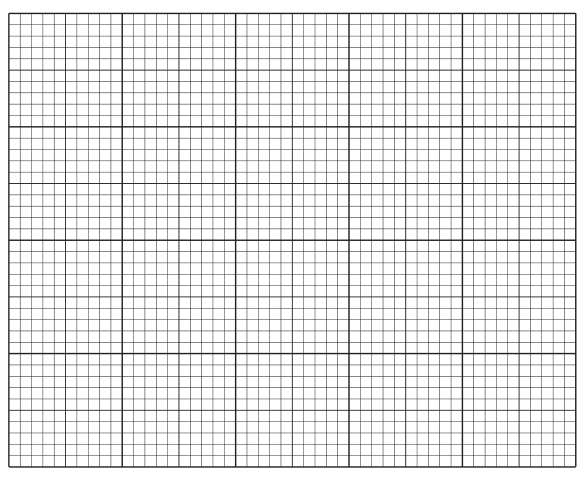
Approach
For the Smarts team, calculate the lower quartile (LQ), median (M), and upper quartile (UQ) from the sorted data. The Teasers' values are already given. Plot both box-and-whisker plots on a single diagram using a linear scale, ensuring all five key values are plotted accurately and labelled.
Working
Smarts data (sorted):
Number of values, .
- Lowest value:
- Lower quartile (LQ): position rd value
- Median (M): position th value
- Upper quartile (UQ): position th value
- Highest value:
Teasers data:
- Lowest value:
- Lower quartile (LQ): (given)
- Median (M): (given)
- Upper quartile (UQ): (given)
- Highest value:
Plot the box-and-whisker plots on a linear scale from to minutes.
Answer
Box-and-whisker plots drawn with Smarts: lowest , LQ , median , UQ , highest . Teasers: lowest , LQ , median , UQ , highest .
Smarts: lowest 9, Q1 13, median 22, Q3 30, highest 41; Teasers: lowest 12, Q1 18, median 25, Q3 37, highest 39.
Walkthrough
First, identify the five key values (lowest, lower quartile, median, upper quartile, highest) for both teams. For Teasers, these are given as . For Smarts, use the sorted data: . With , the quartile positions are calculated using and . This gives LQ at the 3rd value (), median at the 6th value (), and UQ at the 9th value ().
Next, draw a horizontal axis labelled 'time in minutes' on a linear scale, for example from to . Plot the two box-and-whisker plots on this axis. For each plot, draw a box from the lower quartile to the upper quartile, with a vertical line at the median. Extend whiskers from the box to the lowest and highest values. Label all five key values and the team names.
Key Takeaways
- Box-and-whisker plots summarise data using five key values: minimum, lower quartile, median, upper quartile, and maximum.
- When comparing two distributions, they should be plotted on the same scale to allow direct visual comparison.
- Quartiles can be found using position formulas based on the number of data points.
Common Mistakes
- Calculating quartiles incorrectly (e.g., using instead of ).
- Drawing whiskers through the box or at the corners instead of at the ends of the box.
- Using different scales for each plot or forgetting to label the axis and values.
Things to Be Careful About
- Ensure the scale is linear and clearly labelled with at least three values.
- Whiskers must not go through the box; they start at the ends of the box and go to the minimum/maximum values.
- Both plots must be on the same diagram with a single linear scale.
Approach
Compare the two box-and-whisker plots in terms of central tendency (median) and spread (interquartile range or range). State the comparisons in the context of the problem (times taken to complete the puzzle).
Working
Central tendency:
The median time for Smarts is minutes, while the median time for Teasers is minutes. Since , the Smarts team is quicker on average.
Spread:
The interquartile range (IQR) for Smarts is minutes. The IQR for Teasers is minutes. Since , the Smarts team's times are more consistent (less variable).
Alternatively, the range for Smarts is minutes, and for Teasers is minutes. However, the IQR is a better measure of spread as it is not affected by outliers.
Answer
- Smarts are quicker (lower median time).
- Smarts' times are more consistent (smaller interquartile range).
Smarts are quicker (lower median) and their times are more consistent (smaller IQR).
Walkthrough
To make comparisons between the two teams, look at the box-and-whisker plots for measures of central tendency and spread.
For central tendency, compare the medians. The median time for Smarts is minutes and for Teasers is minutes. Since the Smarts have a lower median time, they are quicker at completing the puzzle.
For spread, compare the interquartile ranges (IQR), which measure the spread of the middle of the data. The IQR for Smarts is minutes. The IQR for Teasers is minutes. Since the Smarts have a smaller IQR, their times are more consistent (less variable) than the Teasers.
Key Takeaways
- Box-and-whisker plots allow for easy comparison of central tendency (median) and spread (IQR or range).
- Always make comparisons in the context of the problem (e.g., 'quicker' or 'more consistent').
- The IQR is often a better measure of spread than the range because it is not affected by extreme values.
Common Mistakes
- Making comparisons without using the correct statistical terms (e.g., saying 'Smarts are faster' without referencing the median).
- Comparing the range instead of the IQR when outliers might be present (though here both can be used, IQR is preferred).
- Forgetting to state the comparison in context.
Things to Be Careful About
- Ensure both comparisons are valid and supported by the data.
- One comparison should be about central tendency and the other about spread.
- Use context-appropriate language (e.g., 'quicker' for time, 'consistent' for spread).
A darts club has 12 members made up of 7 men and 5 women.
Every Monday, a team of 4 is chosen at random to represent the club in a competition.
Find the probability that, on a particular Monday, the team consists of 1 man and 3 women.
Approach
Count the number of possible teams that contain exactly 1 man and 3 women, count the total number of 4-person teams, then divide the favourable number by the total number.
Working
Number of ways to choose 1 man from 7 and 3 women from 5:
Total number of possible teams of 4 from 12 members:
Therefore the required probability is
Answer
14/99 (approx 0.1414)
Walkthrough
A team is chosen at random, so all possible teams are equally likely. We therefore count favourable teams and divide by the total number of teams.
For a favourable team, we need 1 of the 7 men and 3 of the 5 women. These choices are independent, so multiply: . This counts each team once because order within the team does not matter.
Then find the total number of possible teams: choose any 4 members from the 12, giving .
The probability is therefore , which simplifies to , or about .
Key Takeaways
- Random selection with equally likely outcomes uses probability .
- Unordered selections are counted with combinations.
- Simplifying the final fraction is part of presenting the answer clearly.
Common Mistakes
- Using permutations instead of combinations, which double-counts because team order is irrelevant.
- Forgetting to choose the 3 women, or not using the 5 women in the numerator.
- Leaving the probability as without simplifying to or giving .
- Giving an unsupported final answer; a correct answer without method may not earn method marks.
Things to Be Careful About
- The total number of teams is , not , because the order of members in a team does not matter.
- The answer can be given as a fraction or a decimal; both forms are acceptable, but the fraction is exact.
Every Tuesday, the darts club chooses 3 teams of 4. Each team enters a competition in a different town.
In how many different ways can the teams be chosen if there are no restrictions?
Approach
Because the three teams play in different towns, label the teams as Town 1, Town 2 and Town 3. Choose 4 members for Town 1, then choose 4 of the remaining members for Town 2; the last 4 members form Town 3. Multiply the numbers of choices.
Working
Choose the first team:
After the first team is chosen, 8 members remain, so the second team can be chosen in
The remaining 4 members form the third team:
Thus the total number of ways is
Answer
34650
Walkthrough
The differences between the towns make the three teams distinguishable. Name the teams A, B and C. First choose the 4 members for team A from all 12; this leaves 8 members. Then choose team B from those 8; the remaining 4 automatically form team C. Every choice for team A can be paired with every choice for team B, so the numbers of choices are multiplied.
This is why we use rather than dividing by .
Key Takeaways
- Sequential selection from a decreasing pool uses a product of combinations.
- When the teams are distinguishable, such as by town, different assignments are counted separately.
Common Mistakes
- Dividing by : this would be correct only if the three teams were interchangeable, but here they enter competitions in different towns.
- Omitting ; it is harmless but should be shown for a complete method.
Things to Be Careful About
- The question says with no restrictions, so the full product applies.
- If the teams were unlabelled sets, the answer would be , but that is not the situation in this part.
In how many different ways can the teams be chosen if each team must contain at least 1 man and at least 1 woman?
Approach
Every team must contain both men and women, so each team is one of , or . Let , and be the numbers of these three types among the 3 teams. Solve for the possible distributions, count each distribution, and add the results.
Working
Subtracting the first equation from the second gives . The only non-negative integer solutions are:
- , , : one team and two teams;
- , , : two teams and one team.
For the first distribution:
For the second distribution:
These cases are disjoint, so the required total is
Answer
27300
Walkthrough
A valid team of four using both genders can only be , or . Let their counts be , and . There are three teams, so . The total number of men is 7, so . Subtracting the first equation from the second gives . The valid non-negative solutions are and .
For , there is one team with 3 men and 1 woman and two identical teams with 2 men and 2 women. Choose the team first: . From the remaining 4 men and 4 women, choose one of the teams: . The remaining members form the other team. Since the two teams have identical composition, assigning the three team types to the three towns gives choices.
For , there are two identical teams and one team. Choose the first team, then choose the second from the remaining 4 men and 4 women; the leftover members form the team. Again multiply by for the two identical compositions.
The two distributions cannot overlap, so add the counts.
Key Takeaways
- When several compositions are possible, enumerate all valid distributions first.
- For repeated identical team compositions, account for the repetitions when assigning teams to towns.
- Disjoint cases should be added.
Common Mistakes
- Missing one of the two possible distributions.
- Treating the two identical teams as distinct, which overcounts by a factor of 2.
- Not reducing the pool after choosing the first team, causing repeated selections of the same people.
- Dividing the final total by : that would give 4550, the answer for unlabelled teams, not for teams entering different towns.
Things to Be Careful About
- The teams are in different towns, so they are labelled; the order of the four members within a team does not matter.
- Check that each distribution uses exactly 7 men and 5 women in total.
- The direct enumeration method avoids the inclusion-exclusion pitfalls of subtracting invalid cases.
The 7 men stand in a line for a photograph. Two of them are brothers, George and Harry.
How many different arrangements are there of the 7 men in which there are exactly 2 men between George and Harry?
Approach
Use a block method. George and Harry must be the two ends of a 4-person block with exactly two men between them. Choose and order the two men between them, arrange the brothers at the two ends, then treat the block as one item along with the remaining 3 men.
Working
Choose and order two men from the other 5 men to stand between George and Harry:
George and Harry can be arranged at the two ends of the block in ways. Now treat the block as one object; together with the remaining 3 men there are 4 objects to arrange:
Therefore the total number of arrangements is
Answer
960
Walkthrough
The condition exactly two men between George and Harry means George and Harry occupy the two ends of a group of four men. The two men between them can be chosen and ordered from the five men other than George and Harry; use because their order matters.
George could be on the left and Harry on the right, or vice versa, giving choices. The four men George, X, Y, Harry form one fixed block. Combine this block with the remaining 3 men, giving 4 objects to arrange in a line, which can be done in ways.
Multiplying these independent choices gives the total number of valid arrangements.
Key Takeaways
- The block method is useful when certain people must appear together with a fixed number of people between them.
- Permutations count both selection and order, so is appropriate for the two men between the brothers.
- Arrangements inside the block and arrangements of the block with other people are independent and are multiplied.
Common Mistakes
- Using combinations for the two men between George and Harry, which ignores their order; the two possible orders are different arrangements.
- Forgetting that George and Harry can be swapped.
- Treating George and Harry as if they are included among the 5 people from whom the two middle men are chosen; actually there are only 5 other men available.
Things to Be Careful About
- The block contains 4 people: George, two other men, and Harry.
- There are 3 remaining men outside the block, so the block and the remaining men form 4 objects.
- The phrase exactly 2 men between excludes adjacent arrangements and arrangements with 1, 3 or 4 men between the brothers.