9709/65 Oct/Nov 2025 — Mathematics Solved Past Paper

Q1Medium-EasySampling and Estimation

A student notes the length, $t$ minutes, of certain lectures. The results for a random sample of 80 lectures are summarised as follows.

n = 80 \qquad \Sigma t = 6430 \qquad \Sigma t^2 = 519\,740

(a)

Calculate a 96% confidence interval for the population mean length of the lectures.

6M Similar

DifficultyMedium-Easy

Worked solution

Approach

Since $n=80$ is large, the Central Limit Theorem ensures the sample mean $\bar t$ is approximately normally distributed. We estimate the population mean and variance from the sample, then form a two-sided 96% confidence interval using the critical value $z = 2.054$ .

Working

The sample mean is

\bar t = \frac{\sum t}{n} = \frac{6430}{80} = 80.375

The unbiased estimate of the population variance is

s^2 = \frac{n}{n-1}\left(\frac{\sum t^2}{n} - \bar t^2\right) = \frac{80}{79}\left(\frac{519740}{80} - 80.375^2\right) = 37.073

The standard error of the sample mean is

\sqrt{\frac{s^2}{n}} = \sqrt{\frac{37.073}{80}} = 0.6807

For a 96% confidence interval, the total tail probability is 4%, so each tail is 2%, giving $z = 2.054$ .

The confidence interval is

80.375 \pm 2.054 \times 0.6807

= 80.375 \pm 1.398

= (78.977, 81.773)

Answer

The 96% confidence interval for the mean lecture length is $79.0$ to $81.8$ minutes (3 s.f.).

Final answer

79.0 to 81.8 minutes (3 s.f.)

Detailed explanation

Walkthrough

First, calculate the sample mean $\bar t = \frac{6430}{80} = 80.375$ ; this is the point estimate of the population mean.

Next, calculate the unbiased estimate of the population variance. Because the sample variance with denominator $n$ is biased, multiply by $\frac{n}{n-1}$ , i.e. use

s^2 = \frac{n}{n-1}\left(\frac{\sum t^2}{n} - \bar t^2\right)

This gives $37.073$ for the variance estimate.

Then identify the critical value for a 96% confidence interval. Since the total tail probability is 4%, and there are two tails, each tail is 2%, so the required $z$ -value is $2.054$ .

Finally, substitute into the confidence interval formula

\bar t \pm z \sqrt{\frac{s^2}{n}}

using $n=80$ , giving the interval $79.0$ to $81.8$ minutes. Each of these steps corresponds to a mark: the estimate of the mean (B1), the unbiased variance calculation (M1 A1), the correct $z$ (B1), the interval formula (M1), and the final interval (A1).

Key Takeaways

This question tests the large-sample confidence interval for a population mean. The key ideas are the Central Limit Theorem, the use of an unbiased variance estimate $s^2$ , and the correct critical value for the confidence level.

Common Mistakes

Using the biased variance $\frac{\sum t^2}{n} - \bar t^2$ instead of multiplying by $\frac{n}{n-1}$ . The mark scheme awards M0 A0 if a biased variance is used.
Using $z = 1.96$ for a 96% interval; the correct value is about $2.054$ .
Forgetting to divide the variance by $n$ before taking the square root.
Quoting a point instead of an interval for the final answer.

Things to Be Careful About

Keep enough decimal places in intermediate steps; rounding $80.375^2$ too early can change the final interval.
The mark scheme accepts $z = 2.054$ or $2.055$ .
Give the final interval to 3 significant figures: $79.0$ to $81.8$ .

Techniques used

Calculate sample meanCalculate unbiased estimate of population varianceFind critical z-value for a specified confidence levelConstruct confidence interval for population mean

(b)

The method used in part (a) is valid because the sample size was large. Explain why the method would not be valid if the sample size were small.

1M Similar

Q2Medium-EasyHypothesis Tests

A researcher is investigating whether the proportion of families who do not own a car in his town is different from the proportion of the population in the whole country, which is 10.1%. He takes a large random sample of families in his town and finds the proportion of families that do not own a car.

(a)

Explain why a two-tailed test is appropriate in this context.

1M Similar

DifficultyEasy

Worked solution

Approach

A two-tailed test is used when the alternative hypothesis does not specify a direction. Here the researcher is only investigating whether the town proportion is different from the national proportion, not whether it is greater or less.

Working

The claim under investigation is that the proportion in the town is different from the national proportion. This could mean the town proportion is greater than 10.1% or less than 10.1%. Therefore the rejection region must be split between the two tails of the distribution.

Answer

A two-tailed test is appropriate because the researcher is looking for evidence that the proportion is different from 10.1%, not specifically greater than or less than 10.1%.

Final answer

A two-tailed test is appropriate because the researcher is looking for evidence that the proportion is different from 10.1%, not specifically greater or less.

Detailed explanation

Walkthrough

The key word is "different from". It has no direction. If the researcher suspected "greater than", a one-tailed test would be appropriate; if the researcher suspected "less than", a one-tailed test in the other direction would be appropriate. Since the researcher is only asking whether there is a difference, both directions must be considered, so the test is two-tailed.

Key Takeaways

A two-tailed test is used when the alternative hypothesis is of the form "not equal to". The significance level is split between the two tails of the distribution.

Common Mistakes

Using a one-tailed test when the question says "different from".
Thinking that "different" implies greater, or less, rather than either.

Things to Be Careful About

The explanation should make it clear that the choice is based on the absence of a direction in the research question, not on the size of the sample or the value of the test statistic.

Techniques used

recognise that the research question has no directional claimdecide that both tails of the distribution must be considered

(b)

State suitable null and alternative hypotheses for the test.

1M Similar

(c)

The researcher calculates the value of the test statistic $z$ and finds that $z = 1.82$ . He carries out the test at the 5% significance level.

State the conclusion of the test, explaining your answer.

2M Similar

DifficultyMedium-Easy

Worked solution

Approach

For a two-tailed test at the 5% significance level, the critical value is $z = 1.96$ . Compare the observed value $z = 1.82$ with this critical value, then state the conclusion in context.

Working

1.82 < 1.96

The test statistic is not in the critical region. Equivalently, the one-tail probability is $0.0344 > 0.025$ .

Answer

Do not reject $H_0$ . There is insufficient evidence that the proportion of families in the town who do not own a car is different from 10.1%.

Final answer

Do not reject H0; insufficient evidence that the town proportion differs from 10.1%.

Detailed explanation

Walkthrough

At the 5% significance level, a two-tailed test has critical values $z = \pm 1.96$ . The test statistic is $z = 1.82$ . Since $1.82 < 1.96$ , the test statistic lies inside the acceptance region, so the result is not significant.

Equivalently, the probability in one tail beyond $z = 1.82$ is approximately $0.0344$ . For a two-tailed 5% test, each tail has area $0.025$ . Since $0.0344 > 0.025$ , the result is not significant.

Therefore we do not reject $H_0$ . This means there is not enough evidence to say that the town proportion is different from the national proportion of 10.1%.

Key Takeaways

For a two-tailed 5% test, the critical value is $z = 1.96$ .
Compare the test statistic with the critical value to decide whether it lies in the critical region.
The conclusion must be stated in context and should say "insufficient evidence", not "the proportion is equal to 10.1%" as a proven fact.

Common Mistakes

Using 1.645, which is the critical value for a one-tailed 5% test.
Comparing 0.0344 with 0.05 instead of 0.025 in a two-tailed test.
Saying "accept $H_0$ " instead of "do not reject $H_0$ ".
Giving a conclusion without context.

Things to Be Careful About

At the 5% two-tailed level, the critical value is 1.96, not 1.645. The conclusion should not overstate the result: there is insufficient evidence of a difference, not proof that the proportion is exactly 10.1%.

Techniques used

identify the critical value for a two-tailed 5% testcompare the test statistic with the critical valuestate the conclusion in context without overstating the evidence

Q3MediumHypothesis TestsThe Poisson Distribution

A certain website receives an average of $\mu$ hits per hour. In the past the value of $\mu$ was 14.4. After making some improvements, the owner of the website wishes to test whether the value of $\mu$ has increased. He chooses a 10-minute period at random and finds that there were 6 hits during this period. You may assume that the number of hits the website receives in any given time period follows a Poisson distribution.

(a)

Carry out the test at the 2.5% significance level.

6M Similar

DifficultyMedium

Worked solution

Approach

Set up the null and alternative hypotheses for the Poisson mean. Convert the hourly mean to the 10-minute test period, compute the p-value $P(X \geq 6)$ using the Poisson distribution, compare it with the 2.5% significance level, and draw a conclusion in context.

Working

The mean rate is 14.4 hits per hour. Since the test period is 10 minutes, which is $\frac{1}{6}$ of an hour, the mean number of hits in the test period is:

\lambda = \frac{14.4}{6} = 2.4

State the hypotheses:

H_0: \lambda = 2.4 \quad (\text{i.e. } \mu = 14.4)

H_1: \lambda > 2.4 \quad (\text{i.e. } \mu > 14.4)

This is a one-tailed test at the 2.5% significance level. The observed value is 6 hits, so the p-value is:

P(X \geq 6) = 1 - P(X \leq 5)

Using the Poisson distribution with $\lambda = 2.4$ :

P(X \leq 5) = e^{-2.4}\left(1 + 2.4 + \frac{2.4^2}{2!} + \frac{2.4^3}{3!} + \frac{2.4^4}{4!} + \frac{2.4^5}{5!}\right)

= e^{-2.4}(1 + 2.4 + 2.88 + 2.304 + 1.3824 + 0.6636)

= 0.09072 + 0.2177 + 0.2613 + 0.2090 + 0.1254 + 0.060196

= 0.9643

Therefore:

P(X \geq 6) = 1 - 0.9643 = 0.0357 \quad (3 \text{ sf})

Compare with the significance level:

0.0357 > 0.025

Since the p-value is greater than the significance level, we do not reject $H_0$ .

Answer

There is insufficient evidence that the mean number of hits per hour has increased.

Final answer

Do not reject the null hypothesis. There is insufficient evidence that the mean number of hits per hour has increased.

Detailed explanation

Walkthrough

The first step is to recognise that the mean is given per hour (14.4 hits per hour) but the observation is over a 10-minute period. Since 10 minutes is one-sixth of an hour, the expected number of hits in the test period is $14.4 \div 6 = 2.4$ . This conversion is essential — using 14.4 directly would give a completely wrong p-value.

Next, set up the hypotheses. The null hypothesis $H_0$ states that the mean has not changed: $\lambda = 2.4$ (equivalently $\mu = 14.4$ per hour). The alternative hypothesis $H_1$ states that the mean has increased: $\lambda > 2.4$ . This is a one-tailed test because the owner only wants to detect an increase, not a decrease.

The observed value is 6 hits. Since the alternative is $\lambda > 2.4$ , the p-value is the probability of observing 6 or more hits: $P(X \geq 6)$ . We compute this as $1 - P(X \leq 5)$ because it is easier to sum the probabilities from 0 to 5.

The Poisson probability formula gives $P(X = x) = e^{-\lambda}\lambda^x / x!$ . Summing from $x = 0$ to 5 and subtracting from 1 gives the p-value $0.0357$ .

Finally, compare the p-value with the significance level 0.025. Since $0.0357 > 0.025$ , the result is not statistically significant, so we do not reject $H_0$ . The conclusion must be stated in context: there is insufficient evidence that the mean number of hits per hour has increased.

Key Takeaways

When the mean is given for one time period but the observation is over a different period, convert the mean proportionally.
For a one-tailed test with $H_1: \lambda > \lambda_0$ , the p-value is $P(X \geq \text{observed value})$ .
The p-value is compared with the significance level: reject $H_0$ if the p-value is less than the significance level.
The conclusion must be phrased in the context of the problem.

Common Mistakes

Using $\lambda = 14.4$ instead of $\lambda = 2.4$ for the 10-minute period.
Computing $P(X \leq 6)$ instead of $P(X \geq 6)$ — the wrong tail.
Not showing the full Poisson expression; the mark scheme requires the expression $1 - e^{-2.4}(1 + 2.4 + \frac{2.4^2}{2!} + \cdots)$ to be seen for the method mark. An unjustified answer of 0.0357 scores only B1M0B1.
Stating the conclusion without context (e.g., just "do not reject $H_0$ " without mentioning the mean/hits).

Things to Be Careful About

The significance level is 2.5%, which is 0.025.
The comparison must be valid: $0.0357 > 0.025$ , so we do not reject $H_0$ .
The final answer should be given to 3 significant figures (0.0357).

Techniques used

convert the mean rate to the observation periodset up null and alternative hypothesescompute the Poisson tail probabilitycompare the p-value with the significance level

(b)

Explain whether it is possible that a Type I error or a Type II error or both may have been made in carrying out the test.

2M Similar

DifficultyMedium-Easy

Worked solution

Approach

Since $H_0$ was not rejected in part (a), determine which of the two types of error could possibly have been made.

Working

In part (a) we did not reject $H_0$ .

A Type I error is rejecting $H_0$ when it is actually true. Since we did not reject $H_0$ , a Type I error cannot have been made.

A Type II error is failing to reject $H_0$ when it is actually false. Since we did not reject $H_0$ , and it is possible that $H_0$ is false (the mean may have increased without us detecting it), a Type II error may have been made.

Since a Type I error requires rejecting $H_0$ and a Type II error requires not rejecting $H_0$ , both cannot have been made in this single test.

Answer

A Type II error may have been made, but a Type I error cannot have been made. Both cannot have been made.

Final answer

A Type II error may have been made; a Type I error cannot have been made. Both cannot have been made.

Detailed explanation

Walkthrough

In part (a) we did not reject $H_0$ . Now we need to think about which errors are possible given this decision.

A Type I error is defined as rejecting $H_0$ when it is actually true. Since we did not reject $H_0$ , a Type I error cannot have been made — we never made the decision that would constitute a Type I error.

A Type II error is defined as failing to reject $H_0$ when it is actually false. Since we did not reject $H_0$ , and it is entirely possible that $H_0$ is false (the mean may have genuinely increased, but the evidence was not strong enough to detect it), a Type II error may have been made.

Because a Type I error requires the decision "reject $H_0$ " and a Type II error requires the decision "do not reject $H_0$ ", the two errors are mutually exclusive in a single test — both cannot have been made.

Key Takeaways

Type I error: rejecting a true null hypothesis.
Type II error: failing to reject a false null hypothesis.
The two errors are mutually exclusive in a single test outcome.

Common Mistakes

Confusing the two error types.
Claiming both errors may have been made — impossible since they require opposite decisions.
Not linking the reasoning to the fact that $H_0$ was not rejected.

Things to Be Careful About

The mark scheme requires stating that $H_0$ was not rejected (at least once) to justify the reasoning.
The answer must be in context — mention the mean/hits where appropriate.

Techniques used

distinguish Type I and Type II errorsreason about error possibility given the test decision

Q4MediumThe Poisson Distribution

A sports fan produces a magazine each month.

(a)

On average 1 in 540 characters in the magazine is incorrect.

4M

(i)

Use an appropriate approximating distribution to find the probability that, in a magazine containing 2430 characters, there are at least 4 incorrect characters.

3M Similar

DifficultyMedium-Easy

Worked solution

Approach

The number of incorrect characters follows a binomial distribution $X \sim B\left(2430, \frac{1}{540}\right)$ . Since $n$ is large and $p$ is small, we use the Poisson approximation with $\lambda = np$ .

Working

\lambda = np = 2430 \times \frac{1}{540} = 4.5

So $X \sim \text{Po}(4.5)$ . We require $P(X \geq 4)$ :

P(X \geq 4) = 1 - P(X \leq 3)

P(X \leq 3) = e^{-4.5}\left(1 + 4.5 + \frac{4.5^2}{2!} + \frac{4.5^3}{3!}\right)

\frac{4.5^2}{2!} = 10.125, \qquad \frac{4.5^3}{3!} = 15.1875

P(X \leq 3) = e^{-4.5}(1 + 4.5 + 10.125 + 15.1875) = e^{-4.5}(30.8125)

P(X \leq 3) = 0.3423

P(X \geq 4) = 1 - 0.3423 = 0.6577

Answer

P(X \geq 4) = 0.658 \quad (3 \text{ s.f.})

Final answer

0.658

Detailed explanation

Walkthrough

The number of incorrect characters is a binomial random variable, since each of the 2430 characters is independently either correct or incorrect, with probability $p = \frac{1}{540}$ of being incorrect. Computing $P(X \geq 4)$ directly from the binomial formula would be extremely tedious, so we use the Poisson approximation, which is valid because $n$ is large and $p$ is small. The parameter is $\lambda = np = 4.5$ , so we model $X \sim \text{Po}(4.5)$ .

To find $P(X \geq 4)$ , we avoid summing infinitely many terms by using the complement: $P(X \geq 4) = 1 - P(X \leq 3)$ . Each term $P(X = r) = e^{-4.5}\frac{4.5^r}{r!}$ is computed for $r = 0, 1, 2, 3$ and summed. Finally we subtract this sum from 1, giving $0.658$ to 3 significant figures.

Key Takeaways

This question tests the Poisson approximation to the binomial: $B(n, p) \approx \text{Po}(np)$ when $n$ is large and $p$ is small. It also tests computing cumulative Poisson probabilities and using the complement rule for "at least" probabilities.

Common Mistakes

Computing $P(X \leq 3)$ but forgetting to subtract from $1$ to obtain $P(X \geq 4)$ .
Misplacing the factorials: $2! = 2$ and $3! = 6$ .
Trying to sum infinitely many Poisson terms instead of using the complement.
The mark scheme warns that an unjustified answer of $0.658$ scores only B1M0B1 — the full probability expression must be shown.

Things to Be Careful About

Use exactly $\lambda = 4.5$ , obtained from $\frac{2430}{540}$ .
Show the full expression $e^{-4.5}\left(1 + 4.5 + \frac{4.5^2}{2!} + \frac{4.5^3}{3!}\right)$ to earn the M1 mark.
Using $B\left(2430, \frac{1}{540}\right)$ directly with the same answer scores B2, but the Poisson route is the intended one.
Round to 3 significant figures.

Techniques used

apply Poisson approximation to the binomial distributioncompute the parameter as npuse the complement rule for an upper-tail probabilitysum Poisson probability terms

(ii)

Justify your approximating distribution.

1M Similar

(b)

On average the number of copies, $X$ , of the magazine sold per month is 123.4.

6M

(i)

State one condition for $X$ to have a Poisson distribution.

1M Similar

(ii)

You are now given that $X$ has a Poisson distribution.

Use an appropriate approximating distribution to find the probability that in a randomly chosen month, more than 130 copies of the magazine are sold.

5M Similar

DifficultyMedium

Worked solution

Approach

Since $X \sim \text{Po}(123.4)$ has $\lambda = 123.4 > 10$ , we approximate by a normal distribution with $\text{E}(X) = \text{Var}(X) = 123.4$ . We then apply a continuity correction for the strict inequality $X > 130$ and standardise.

Working

X \sim N(123.4,\ 123.4)

"More than 130 copies" means $X \geq 131$ , so with the continuity correction we standardise $130.5$ :

z = \frac{130.5 - 123.4}{\sqrt{123.4}} = \frac{7.1}{11.1086} \approx 0.639

P(X > 130) = P(Z > 0.639) = 1 - \Phi(0.639)

From normal tables, $\Phi(0.639) \approx 0.7386$ , so

P(X > 130) = 1 - 0.7386 = 0.2614

Answer

P(X > 130) = 0.261 \quad (3 \text{ s.f.})

Final answer

0.261

Detailed explanation

Walkthrough

We are told $X$ is Poisson with mean 123.4. When $\lambda$ is large (here $> 10$ ), the Poisson distribution is closely approximated by a normal distribution having the same mean and variance, so $X \sim N(123.4, 123.4)$ . Because $X$ is discrete, the event "more than 130 copies" means $X \geq 131$ ; the continuity correction moves the boundary by 0.5 to 130.5 to bridge the discrete and continuous scales. We then standardise: $z = \frac{130.5 - 123.4}{\sqrt{123.4}} \approx 0.639$ . Since we need the upper tail $P(Z > 0.639) = 1 - \Phi(0.639)$ , we read $\Phi(0.639) \approx 0.7386$ from tables and subtract from 1, giving $0.261$ .

Key Takeaways

The normal approximation to the Poisson, valid when $\lambda$ is large: $\text{Po}(\lambda) \approx N(\lambda, \lambda)$ since mean = variance = $\lambda$ . The continuity correction for a discrete-to-continuous approximation. Standardising: $z = \frac{x - \mu}{\sigma}$ and reading upper-tail probabilities from normal tables.

Common Mistakes

Forgetting the continuity correction and using 130 instead of 130.5. The mark scheme condones wrong or missing cc for M1 only, but you then lose the A1.
Using the wrong variance: for a Poisson variable the variance equals $\lambda = 123.4$ .
Reporting $\Phi(0.639)$ directly instead of $1 - \Phi(0.639)$ for the "more than" tail.

Things to Be Careful About

State $N(123.4, 123.4)$ explicitly — both B1 marks in the mark scheme depend on it (one for the mean, one for the variance).
Use 130.5, not 130, for $P(X > 130)$ .
Make sure your standardising uses the same values you quoted: $\frac{130.5 - 123.4}{\sqrt{123.4}}$ .
Round the final answer to 3 significant figures: 0.261.

Techniques used

approximate a Poisson variable by a normal distributionapply a continuity correction for a discrete-to-continuous approximationstandardise a normal random variablefind an upper-tail probability from normal tables

Q5MediumLinear Combinations of Random Variables

The masses, in kg, of large and small bags of tomatoes have the distributions $L \sim \mathrm{N}(2.10, 0.12)$ and $S \sim \mathrm{N}(1.51, 0.09)$ respectively.

(a)

Find $\mathrm{P}(L > S + 0.5)$ .

5M Similar

DifficultyMedium

Worked solution

Approach

Define the difference $D = L - S$ . Since $L$ and $S$ are independent normal variables, $D$ is also normal. Combine the means by subtraction and the variances by addition, then standardise and use the symmetry of the normal distribution.

Working

Given

L \sim \mathrm{N}(2.10, 0.12), \quad S \sim \mathrm{N}(1.51, 0.09)

Let $D = L - S$ . Then

D \sim \mathrm{N}(2.10 - 1.51, \, 0.12 + 0.09) = \mathrm{N}(0.59, 0.21)

The required probability is

\mathrm{P}(L > S + 0.5) = \mathrm{P}(L - S > 0.5) = \mathrm{P}(D > 0.5)

Standardise:

z = \frac{0.5 - 0.59}{\sqrt{0.21}} = \frac{-0.09}{\sqrt{0.21}} = -0.196

Using symmetry,

\mathrm{P}(Z > -0.196) = 1 - \Phi(-0.196) = \Phi(0.196)

From normal tables,

\Phi(0.196) = 0.578

Answer

\mathrm{P}(L > S + 0.5) = 0.578

Final answer

0.578

Detailed explanation

Walkthrough

We are asked for the probability that a randomly chosen large bag is more than 0.5 kg heavier than a randomly chosen small bag. Because both masses are normally distributed and the bags are chosen independently, the difference $D = L - S$ is also normal.

The mean of a difference is the difference of the means:

\mathrm{E}(D) = 2.10 - 1.51 = 0.59

A common trap is to subtract variances, but for independent variables the variance of a difference is the sum of the variances:

\mathrm{Var}(D) = 0.12 + 0.09 = 0.21

The event $L > S + 0.5$ is the same as $D > 0.5$ . We standardise $D$ by subtracting its mean and dividing by its standard deviation, giving a negative $z$ -score. Because the normal distribution is symmetric, $\mathrm{P}(Z > -0.196) = \mathrm{P}(Z < 0.196)$ , which we read directly from the normal table.

Key Takeaways

A linear combination of independent normal variables is normal.
For a difference of independent variables, means subtract but variances add.
Standardising converts any normal probability into a standard normal probability.
Symmetry lets us handle negative $z$ -scores.

Common Mistakes

Subtracting variances instead of adding them.
Using $\mathrm{P}(D < 0.5)$ instead of $\mathrm{P}(D > 0.5)$ .
Forgetting to divide by the standard deviation when standardising.
Looking up $\Phi(-0.196)$ directly and giving the wrong tail.

Things to Be Careful About

The inequality $L > S + 0.5$ must be rearranged to $L - S > 0.5$ before standardising.
Use the unrounded mean and variance when calculating $z$ .
Give the final probability to 3 significant figures as required.

Techniques used

define difference of independent normal variablescombine means and variances for a differencestandardise a normal variableuse symmetry of the normal distribution

(b)

The price of tomatoes is $4.30 per kg.

A large bag of tomatoes and a small bag of tomatoes are chosen at random. Find the probability that the total price of the tomatoes in the two bags is less than $16.

5M Similar

DifficultyMedium

Worked solution

Approach

Let $W = L + S$ be the total mass. Since $L$ and $S$ are independent normal variables, $W$ is normal. The total price is $T = 4.3W$ , which is also normal. Find the mean and variance of $T$ , then standardise to find $\mathrm{P}(T < 16)$ .

Working

Given

L \sim \mathrm{N}(2.10, 0.12), \quad S \sim \mathrm{N}(1.51, 0.09)

The total mass is

W \sim \mathrm{N}(2.10 + 1.51, \, 0.12 + 0.09) = \mathrm{N}(3.61, 0.21)

The total price is $T = 4.3W$ , so

\mathrm{E}(T) = 4.3 \times 3.61 = 15.523

and

\mathrm{Var}(T) = 4.3^2 \times 0.21 = 18.49 \times 0.21 = 3.8829

Therefore

T \sim \mathrm{N}(15.523, 3.8829)

Standardise:

z = \frac{16 - 15.523}{\sqrt{3.8829}} = \frac{0.477}{\sqrt{3.8829}} = 0.242

So

\mathrm{P}(T < 16) = \Phi(0.242) = 0.596

Answer

The probability that the total price is less than $16 is

0.596

Final answer

0.596

Detailed explanation

Walkthrough

The total price is found by multiplying the total mass by $4.30 per kg. First combine the two masses into a total mass $W = L + S$ . Since $L$ and $S$ are independent normal variables, $W$ is normal with

\mathrm{E}(W) = 2.10 + 1.51 = 3.61, \quad \mathrm{Var}(W) = 0.12 + 0.09 = 0.21

Multiplying a normal variable by a constant keeps it normal. The mean is multiplied by the constant, but the variance is multiplied by the square of the constant:

\mathrm{E}(T) = 4.3 \times 3.61 = 15.523, \quad \mathrm{Var}(T) = 4.3^2 \times 0.21 = 3.8829

So $T \sim \mathrm{N}(15.523, 3.8829)$ . We need $\mathrm{P}(T < 16)$ . Standardise:

z = \frac{16 - 15.523}{\sqrt{3.8829}} = 0.242

Then $\mathrm{P}(T < 16) = \Phi(0.242) = 0.596$ .

An equivalent method is to convert the price limit into a mass limit: the total price is less than $16 exactly when $W < 16/4.3 = 3.7209$ . Standardising this with $W \sim \mathrm{N}(3.61, 0.21)$ gives the same $z = 0.242$ .

Key Takeaways

The sum of independent normal variables is normal.
Scaling a normal variable by a constant preserves normality.
$\mathrm{Var}(aX) = a^2\mathrm{Var}(X)$ , not $a\mathrm{Var}(X)$ .
Probability questions can often be solved in original units or scaled units.

Common Mistakes

Using $4.3 \times 0.21$ instead of $4.3^2 \times 0.21$ for the variance.
Using $4.3(L - S)$ instead of $4.3(L + S)$ .
Forgetting that the total price includes both bags.
Using the wrong tail: the question asks for less than $16.
Rounding the mean or variance before standardising.

Things to Be Careful About

The price per kg is $4.30, so the total price is $4.3$ times the total mass in kg.
If using the alternative method, divide $16 by $4.30 to get the critical mass, not multiply.
Strict inequality does not matter for a continuous normal distribution.
Give the final answer to 3 significant figures.

Techniques used

form total price as a linear combinationcombine means and variances with scalingstandardise a normal variableevaluate normal CDF

Q6MediumContinuous Random Variables

Fig. 1

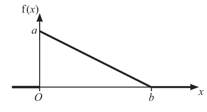
The diagram shows the graph of the probability density function, $\mathrm{f}$ , of a random variable $X$ . The graph is a straight line from $(0, a)$ to $(b, 0)$ where $a$ and $b$ are constants. Elsewhere $\mathrm{f}(x) = 0$ .

(a)

Find an expression for $b$ in terms of $a$ .

2M Similar

DifficultyMedium-Easy

Worked solution

Approach

The probability density function $f(x)$ forms a right-angled triangle with the coordinate axes. Since $f(x)$ is a valid PDF, the total area under the curve must equal 1. Use the formula for the area of a triangle to find $b$ in terms of $a$ .

Working

The graph of $f(x)$ is a straight line from $(0, a)$ to $(b, 0)$ , forming a right-angled triangle with vertices at $(0, 0)$ , $(0, a)$ , and $(b, 0)$ .

The area of this triangle is:

\frac{1}{2} \times \text{base} \times \text{height} = \frac{1}{2} \times b \times a

Since $f(x)$ is a probability density function, the total area must equal 1:

\frac{1}{2} ab = 1

Solving for $b$ :

ab = 2 \implies b = \frac{2}{a}

Answer

b = \frac{2}{a}

Final answer

b = 2/a

Detailed explanation

Walkthrough

A probability density function must satisfy the property that the total area under the curve equals 1. The graph shows $f(x)$ as a straight line from $(0, a)$ on the y-axis to $(b, 0)$ on the x-axis, with $f(x) = 0$ elsewhere. This forms a right-angled triangle with the axes, having base $b$ and height $a$ . The area of this triangle is $\frac{1}{2}ab$ . Setting this equal to 1 gives $\frac{1}{2}ab = 1$ , which rearranges to $b = \frac{2}{a}$ .

Key Takeaways

The total area under any valid PDF equals 1.
For simple geometric shapes (triangles, rectangles), the area can be found using basic geometry rather than integration.
This property is used to find unknown constants in a PDF definition.

Common Mistakes

Forgetting the $\frac{1}{2}$ factor in the triangle area formula.
Using the wrong base or height for the triangle.
Not recognising that $f(x) = 0$ outside $[0, b]$ , so only the triangular region contributes to the area.

Things to Be Careful About

Ensure the area calculation covers only the region where $f(x) > 0$ , which is $0 \leq x \leq b$ .
The constants $a$ and $b$ must both be positive for a valid PDF.

Techniques used

use the area under a PDF equal to 1recognise triangular region under the curve

(b)

Given that $\mathrm{E}(X) = \frac{4}{9}$ find the value of $a$ .

5M Similar

DifficultyMedium

Worked solution

Approach

First, find the equation of the straight line forming the PDF. Substitute $b = \frac{2}{a}$ from part (a) to express $f(x)$ purely in terms of $a$ . Then use the definition $E(X) = \int_0^b x f(x) \, dx$ to set up an equation in $a$ , and solve it using the given value $E(X) = \frac{4}{9}$ .

Working

The straight line passes through $(0, a)$ and $(b, 0)$ . Its equation is:

f(x) = a - \frac{a}{b}x

Substituting $b = \frac{2}{a}$ :

f(x) = a - \frac{a}{2/a}x = a - \frac{a^2}{2}x

The expected value is:

E(X) = \int_0^b x f(x) \, dx = \int_0^{2/a} x\left(a - \frac{a^2}{2}x\right) dx = \int_0^{2/a} \left(ax - \frac{a^2}{2}x^2\right) dx

Integrating:

\left[ \frac{ax^2}{2} - \frac{a^2 x^3}{6} \right]_0^{2/a}

Evaluating at the upper limit $x = \frac{2}{a}$ :

\frac{a}{2} \cdot \left(\frac{2}{a}\right)^2 - \frac{a^2}{6} \cdot \left(\frac{2}{a}\right)^3 = \frac{a}{2} \cdot \frac{4}{a^2} - \frac{a^2}{6} \cdot \frac{8}{a^3} = \frac{2}{a} - \frac{4}{3a}

Simplifying:

\frac{2}{a} - \frac{4}{3a} = \frac{6 - 4}{3a} = \frac{2}{3a}

Given $E(X) = \frac{4}{9}$ :

\frac{2}{3a} = \frac{4}{9}

Cross-multiplying:

18 = 12a \implies a = \frac{18}{12} = \frac{3}{2}

Answer

a = \frac{3}{2}

Final answer

a = 3/2

Detailed explanation

Walkthrough

To find $E(X)$ , we first need the explicit form of $f(x)$ . The line from $(0, a)$ to $(b, 0)$ has gradient $\frac{0 - a}{b - 0} = -\frac{a}{b}$ , so the equation is $f(x) = a - \frac{a}{b}x$ . From part (a), $b = \frac{2}{a}$ , so $\frac{a}{b} = \frac{a}{2/a} = \frac{a^2}{2}$ . Thus $f(x) = a - \frac{a^2}{2}x$ for $0 \leq x \leq \frac{2}{a}$ .

The expected value formula is $E(X) = \int_0^b x f(x) \, dx$ . Substituting $f(x)$ and the upper limit $b = \frac{2}{a}$ :

$E(X) = \int_0^{2/a} \left(ax - \frac{a^2}{2}x^2\right) dx = \left[\frac{ax^2}{2} - \frac{a^2 x^3}{6}\right]_0^{2/a}$

At $x = \frac{2}{a}$ : $\frac{a}{2} \cdot \frac{4}{a^2} = \frac{2}{a}$ and $\frac{a^2}{6} \cdot \frac{8}{a^3} = \frac{4}{3a}$ . The difference is $\frac{2}{a} - \frac{4}{3a} = \frac{2}{3a}$ .

Setting $\frac{2}{3a} = \frac{4}{9}$ and solving gives $a = \frac{3}{2}$ .

Key Takeaways

The expected value of a continuous random variable is $E(X) = \int x f(x) \, dx$ .
When the PDF contains unknown parameters, you may need to use multiple properties (area = 1, given mean) to solve for them.
Substitution of results from earlier parts is essential.

Common Mistakes

Forgetting to multiply by $x$ when computing $E(X)$ — integrating $f(x)$ instead of $x f(x)$ gives $P(X \leq b) = 1$ , not the mean.
Algebra errors when substituting $b = \frac{2}{a}$ into $\frac{a}{b}$ .
Incorrect integration of $x^2$ terms.

Things to Be Careful About

The upper limit of integration is $b = \frac{2}{a}$ , not a fixed number.
Ensure all terms are simplified correctly when combining fractions with $a$ in the denominator.

Techniques used

find equation of straight line from two pointssubstitute b in terms of a into f(x)evaluate integral of xf(x) for expected valuesolve equation involving parameter a

(c)

Using the value of $a$ found in part (b) find the value of $k$ such that $\mathrm{P}(X < k) = \frac{3}{4}$ .

4M Similar

DifficultyMedium

Worked solution

Approach

With $a = \frac{3}{2}$ found in part (b), determine the full PDF and compute $b = \frac{4}{3}$ . Set up the equation $P(X < k) = \int_0^k f(x) \, dx = \frac{3}{4}$ , solve the resulting quadratic for $k$ , and reject any value outside the domain $0 \leq x \leq b$ .

Working

From part (b), $a = \frac{3}{2}$ and $b = \frac{2}{a} = \frac{2}{3/2} = \frac{4}{3}$ .

The PDF is:

f(x) = \frac{3}{2} - \frac{9}{8}x, \quad 0 \leq x \leq \frac{4}{3}

We need $P(X < k) = \frac{3}{4}$ :

\int_0^k \left(\frac{3}{2} - \frac{9}{8}x\right) dx = \frac{3}{4}

Integrating:

\left[ \frac{3}{2}x - \frac{9}{16}x^2 \right]_0^k = \frac{3}{2}k - \frac{9}{16}k^2

Setting equal to $\frac{3}{4}$ :

\frac{3}{2}k - \frac{9}{16}k^2 = \frac{3}{4}

Multiplying through by 16:

24k - 9k^2 = 12

Rearranging:

9k^2 - 24k + 12 = 0

Dividing by 3:

3k^2 - 8k + 4 = 0

Factoring:

(3k - 2)(k - 2) = 0

So $k = \frac{2}{3}$ or $k = 2$ .

Since $k$ must lie within the domain of the PDF, $0 \leq k \leq b = \frac{4}{3}$ . The value $k = 2$ exceeds $\frac{4}{3}$ and is therefore rejected.

Thus $k = \frac{2}{3}$ .

Answer

k = \frac{2}{3}

Final answer

k = 2/3

Detailed explanation

Walkthrough

With $a = \frac{3}{2}$ and $b = \frac{4}{3}$ , the PDF is fully determined: $f(x) = \frac{3}{2} - \frac{9}{8}x$ for $0 \leq x \leq \frac{4}{3}$ .

The probability $P(X < k)$ is the area under the PDF from 0 to $k$ . Setting up the integral:

$P(X < k) = \int_0^k \left(\frac{3}{2} - \frac{9}{8}x\right) dx = \left[\frac{3}{2}x - \frac{9}{16}x^2\right]_0^k = \frac{3}{2}k - \frac{9}{16}k^2$

Setting this equal to $\frac{3}{4}$ and multiplying by 16 to clear denominators:

$24k - 9k^2 = 12 \implies 3k^2 - 8k + 4 = 0$

Factoring gives $(3k - 2)(k - 2) = 0$ , so $k = \frac{2}{3}$ or $k = 2$ .

Since the PDF is only defined for $0 \leq x \leq \frac{4}{3}$ , we must have $k \leq \frac{4}{3}$ . The value $k = 2$ is outside this range, so we reject it. The answer is $k = \frac{2}{3}$ .

Key Takeaways

$P(X < k) = \int_0^k f(x) \, dx$ for a PDF defined on $[0, b]$ .
When solving for a probability boundary, always check that the solution lies within the valid domain of the PDF.
Quadratic equations from probability problems often have two roots, but only one may be physically meaningful.

Common Mistakes

Forgetting to check whether the solutions for $k$ lie within the domain $[0, b]$ .
Accepting $k = 2$ without verification, even though $f(x) = 0$ for $x > \frac{4}{3}$ .
Algebra errors when clearing denominators or factoring the quadratic.

Things to Be Careful About

The domain restriction $k \leq b = \frac{4}{3}$ is crucial. Without it, both roots would appear valid.
Ensure the integral limits are correct: from 0 to $k$ , not from $k$ to $b$ .
The value $k = \frac{2}{3}$ is indeed less than $\frac{4}{3}$ , confirming it is valid.

Techniques used

substitute known values into PDF equationset up integral equation for cumulative probabilityform and solve quadratic equationcheck solution against domain of PDF

Mathematics 9709/65 — October/November 2025

Approach

Working

Answer

Walkthrough

Key Takeaways

Common Mistakes

Things to Be Careful About

Approach

Working

Answer

Walkthrough

Key Takeaways

Common Mistakes

Things to Be Careful About

Approach

Working

Answer

Walkthrough

Key Takeaways

Common Mistakes

Things to Be Careful About

Approach

Working

Answer

Walkthrough

Key Takeaways

Common Mistakes

Things to Be Careful About

Approach

Working

Answer

Walkthrough

Key Takeaways

Common Mistakes

Things to Be Careful About

Approach

Working

Answer

Walkthrough

Key Takeaways

Common Mistakes

Things to Be Careful About

Approach

Working

Answer

Walkthrough

Key Takeaways

Common Mistakes

Things to Be Careful About

Approach

Working

Answer

Walkthrough

Key Takeaways

Common Mistakes

Things to Be Careful About

Approach

Working

Answer

Walkthrough

Key Takeaways

Common Mistakes

Things to Be Careful About

Approach

Working

Answer

Walkthrough

Key Takeaways

Common Mistakes

Things to Be Careful About

Approach

Working

Answer

Walkthrough

Key Takeaways

Common Mistakes

Things to Be Careful About

Approach

Working