9709/65 May/June 2025 — Mathematics Solved Past Paper

Q1MediumThe Poisson DistributionLinear Combinations of Random Variables

The random variable $X$ has the distribution $\text{Po}(1.5)$ . The sum of three independent values of $X$ is denoted by $S$ .

(a)

Find $P(S \le 3)$ .

3M Similar

DifficultyMedium-Easy

Worked solution

Approach

Since $S$ is the sum of three independent values of $X$ , and $X \sim \mathrm{Po}(1.5)$ , we have $S \sim \mathrm{Po}(4.5)$ . To find $\mathrm{P}(S \le 3)$ , add the probabilities for $S = 0, 1, 2, 3$ .

Working

S \sim \mathrm{Po}(4.5)

\begin{aligned} \mathrm{P}(S \le 3) &= \mathrm{e}^{-4.5}\left(1 + 4.5 + \frac{4.5^2}{2!} + \frac{4.5^3}{3!}\right) \\ &= \mathrm{e}^{-4.5}(1 + 4.5 + 10.125 + 15.1875) \\ &= 0.01111 + 0.04999 + 0.11248 + 0.16872 \\ &= 0.342 \quad (3\text{ sf}) \end{aligned}

Answer

\mathrm{P}(S \le 3) = 0.342 \quad (3\text{ sf})

Final answer

0.342 (3 sf)

Detailed explanation

Walkthrough

First, identify the distribution of $S$ . Since $X \sim \mathrm{Po}(1.5)$ and $S$ is the sum of three independent values of $X$ , $S \sim \mathrm{Po}(4.5)$ . This is because the sum of independent Poisson variables is Poisson with mean equal to the sum of the means.

To find $\mathrm{P}(S \le 3)$ , we need $\mathrm{P}(S=0)+\mathrm{P}(S=1)+\mathrm{P}(S=2)+\mathrm{P}(S=3)$ . Using the Poisson formula $\mathrm{P}(S=r)=\mathrm{e}^{-4.5}\frac{4.5^r}{r!}$ , each term contributes:

\mathrm{e}^{-4.5}\left(1 + 4.5 + \frac{4.5^2}{2!} + \frac{4.5^3}{3!}\right)

Evaluate the fractions: $\frac{4.5^2}{2!}=10.125$ and $\frac{4.5^3}{3!}=15.1875$ . Then multiply each term by $\mathrm{e}^{-4.5}$ and add to get $0.342$ to 3 significant figures.

Key Takeaways

The sum of independent Poisson random variables is Poisson, with parameter equal to the sum of the individual parameters. A cumulative Poisson probability is found by summing individual probabilities from $0$ up to the required value.

Common Mistakes

Using $\mathrm{Po}(1.5)$ instead of $\mathrm{Po}(4.5)$ for $S$ . Missing the $S=0$ term in the cumulative sum. Rounding intermediate values too early. In the mark scheme, an unsupported answer of $0.342$ only scores one mark, so the expression must be shown.

Things to Be Careful About

The mean of $S$ is $3 \times 1.5 = 4.5$ , not $1.5$ . Include all terms $S=0,1,2,3$ . Give the final answer to 3 significant figures. Show the Poisson expression to earn full marks.

Techniques used

recognise that the sum of independent Poisson variables is Poissoncompute a cumulative Poisson probability by summing individual terms

(b)

Show that the exact value of $\frac{P(S \le 2)}{P(S \le 1)}$ is $\frac{125}{44}$ .

3M Similar

DifficultyMedium

Worked solution

Approach

Write down the cumulative probabilities up to 1 and up to 2 for $\mathrm{Po}(4.5)$ , then divide the two expressions exactly.

Working

\mathrm{P}(S \le 1) = \mathrm{e}^{-4.5}(1 + 4.5) = 5.5\mathrm{e}^{-4.5}

\mathrm{P}(S \le 2) = \mathrm{e}^{-4.5}\left(1 + 4.5 + \frac{4.5^2}{2}\right) = \mathrm{e}^{-4.5}(1 + 4.5 + 10.125) = \frac{125}{8}\mathrm{e}^{-4.5}

Divide:

\frac{\mathrm{P}(S \le 2)}{\mathrm{P}(S \le 1)} = \frac{\frac{125}{8}\mathrm{e}^{-4.5}}{5.5\mathrm{e}^{-4.5}} = \frac{125}{8} \div \frac{11}{2} = \frac{125}{8} \times \frac{2}{11} = \frac{125}{44}

Answer

\frac{\mathrm{P}(S \le 2)}{\mathrm{P}(S \le 1)} = \frac{125}{44}

Final answer

125/44

Detailed explanation

Walkthrough

We need the exact ratio $\frac{\mathrm{P}(S \le 2)}{\mathrm{P}(S \le 1)}$ . First write both cumulative probabilities using $\lambda = 4.5$ .

For $\mathrm{P}(S \le 1)$ :

\mathrm{P}(S \le 1) = \mathrm{e}^{-4.5}(1 + 4.5) = 5.5\mathrm{e}^{-4.5}

For $\mathrm{P}(S \le 2)$ :

\mathrm{P}(S \le 2) = \mathrm{e}^{-4.5}\left(1 + 4.5 + \frac{4.5^2}{2}\right) = \mathrm{e}^{-4.5}(1 + 4.5 + 10.125) = \frac{125}{8}\mathrm{e}^{-4.5}

The factor $\mathrm{e}^{-4.5}$ cancels when we divide. Since $5.5 = \frac{11}{2}$ , dividing by $\frac{11}{2}$ is the same as multiplying by $\frac{2}{11}$ :

\frac{\frac{125}{8}}{\frac{11}{2}} = \frac{125}{8} \times \frac{2}{11} = \frac{125}{44}

This is the exact value required.

Key Takeaways

When taking ratios of Poisson probabilities, the common exponential factor cancels, so exact fractions can be used. The sum of independent Poisson variables is Poisson, so $S \sim \mathrm{Po}(4.5)$ .

Common Mistakes

Using the wrong parameter for $S$ . Omitting the $S=0$ term in either cumulative probability. Using decimals too early and failing to obtain the exact fraction $\frac{125}{44}$ . Not showing both cumulative expressions and the division, which are required by the mark scheme.

Things to Be Careful About

This is a "show that" question, so the final answer must be exact and convincingly obtained. The mark scheme requires both $\mathrm{P}(S \le 1)$ and $\mathrm{P}(S \le 2)$ expressions, with no end error and $\lambda = 4.5$ , before the division is attempted. Avoid decimal approximations in the working.

Techniques used

recognise that the sum of independent Poisson variables is Poissonform cumulative Poisson probability expressionssimplify an exact ratio by cancelling the common exponential factor

Q2MediumSampling and Estimation

A random sample of 200 values of a random variable $X$ gives the following results.

n = 200 \quad \sum(x - 2) = 60 \quad \sum(x - 2)^2 = 20

(a)

Find a 95% confidence interval for the population mean of $X$ .

6M Similar

DifficultyMedium

Worked solution

Approach

Let $Y = X - 2$ . The coded sums are $\sum y = 60$ and $\sum y^2 = 20$ . Estimate the mean and unbiased variance of $X$ , then form a 95% confidence interval using $z = 1.96$ .

Working

Estimate the mean:

\bar{x} = 2 + \frac{60}{200} = 2.3

Estimate the unbiased variance of $Y$ (and hence of $X$ ):

s^2 = \frac{1}{199}\left(20 - \frac{60^2}{200}\right) = \frac{1}{199}(20 - 18) = \frac{2}{199} = 0.01005\ldots

The 95% confidence interval is:

\bar{x} \pm 1.96 \sqrt{\frac{s^2}{n}} = 2.3 \pm 1.96 \sqrt{\frac{0.01005}{200}}

Compute the margin:

1.96 \sqrt{\frac{0.01005}{200}} = 1.96(0.007089\ldots) = 0.01389\ldots

So the interval is:

2.3 - 0.0139 = 2.2861, \qquad 2.3 + 0.0139 = 2.3139

Answer

2.29 < \mu < 2.31 \quad (3\text{ s.f.})

Final answer

2.29 to 2.31 (3 s.f.)

Detailed explanation

Walkthrough

The data are given in coded form: instead of listing the $x$ -values, we are told $\sum(x-2)$ and $\sum(x-2)^2$ . This is a common way to simplify calculations. Define $Y = X - 2$ . Then $\bar{Y} = 60/200 = 0.3$ , so the estimate of the mean of $X$ is $2 + 0.3 = 2.3$ .

Next, estimate the variance. The sample variance formula uses $\sum y^2 - n\bar{y}^2$ . Since we need an unbiased estimate, divide by $n-1 = 199$ . This gives

s^2 = \frac{1}{199}(20 - 200(0.3)^2) = \frac{2}{199} = 0.01005\ldots

Adding a constant to a variable does not change its variance, so this is also the unbiased estimate of the variance of $X$ .

For a 95% confidence interval, use $\bar{x} \pm z \sqrt{s^2/n}$ with $z = 1.96$ . The sample size is large, so the sample mean is approximately normal by the Central Limit Theorem. Substituting gives

2.3 \pm 1.96\sqrt{0.01005/200} = 2.3 \pm 0.0139

so the interval is $(2.2861, 2.3139)$ , which rounds to $(2.29, 2.31)$ .

Key Takeaways

Coded data $\sum(x-a)$ and $\sum(x-a)^2$ can be used to find the sample mean and variance.
The unbiased variance estimate uses divisor $n-1$ .
A confidence interval for the mean has the form $\bar{x} \pm z\sqrt{s^2/n}$ .
For large samples, the CLT justifies using the normal $z$ -value even when the population distribution is unknown.

Common Mistakes

Using the biased variance (dividing by $n$ instead of $n-1$ ); the mark scheme gives M0 for a biased estimate.
Forgetting to add 2 back when converting $\bar{Y}$ to $\bar{X}$ .
Using a $t$ -value or the wrong $z$ -value instead of $1.96$ for 95% confidence.
Giving only one endpoint of the interval instead of the full interval.

Things to Be Careful About

The variance estimate must be unbiased: use $\frac{1}{n-1}\left(\sum y^2 - \frac{(\sum y)^2}{n}\right)$ .
The expression $\frac{60^2}{200}$ is $n\bar{y}^2$ ; do not forget the division by $n$ .
The final answer must be an interval, not just a point estimate.
Rounding to 3 significant figures gives $2.29$ to $2.31$ ; keep more decimal places in intermediate working.
If the biased variance $0.01$ is used, the mark scheme allows at most 4 of the 6 marks.

Techniques used

estimate the mean from coded datacompute the unbiased sample varianceapply the normal confidence interval formulause the 95% z-value

(b)

State which part of your solution to part (a) makes use of the Central Limit Theorem.

1M Similar

Q3Medium-EasySampling and Estimation

Maroulla’s calculator can generate random numbers between 0.000 and 0.999 inclusive, correct to 3 significant figures. She plans to use her calculator to choose a sample of members from the 851 members in her health club. She numbers the members from 1 to 851. Then she uses her calculator to generate some random numbers. She multiplies each random number by 851 and rounds up to the next whole number to give the number of a member in the sample. This is called a ‘member number’.

(a)

Maroulla’s first random number is 0.401.

Find the member number that is produced by this random number.

1M Similar

(b)

Find all possible random numbers, correct to 3 decimal places, that would produce the following member numbers.

2M

(i)

A member number of 680.

1M Similar

DifficultyMedium-Easy

Worked solution

Approach

Work backwards from the member number. A member number of 680 is obtained when the scaled value $851x$ is greater than 679 and not more than 680, because rounding up sends every value in $(679, 680]$ to 680. Solve this inequality for $x$ , then list the possible values that can be written correct to 3 decimal places.

Working

For member number 680:

679 < 851x \le 680

Dividing by 851:

\frac{679}{851} < x \le \frac{680}{851}

So:

0.79788\ldots < x \le 0.79906\ldots

The random numbers correct to 3 decimal places in this interval are:

0.798 \text{ and } 0.799

Answer

0.798 \text{ and } 0.799

Final answer

0.798, 0.799

Detailed explanation

Walkthrough

We need the values of the random number $x$ such that rounding $851x$ up gives 680. If $851x = 679.1$ , then rounding up gives 680; if $851x = 680$ , rounding up also gives 680. However, if $851x = 679$ exactly, rounding up gives 679. So the condition is $679 < 851x \le 680$ .

Dividing each part by 851 gives the interval $0.79788\ldots < x \le 0.79906\ldots$ . The calculator can produce numbers correct to 3 decimal places, so we list the three-decimal values inside this interval. $0.797$ is too small because $851 \times 0.797$ is below 679 and would round up to 679. $0.798$ and $0.799$ both lie in the interval. $0.800$ is too large because it would round up to 681. Thus only those two values work.

Key Takeaways

This part shows how to invert a ‘round up’ mapping: for a member number $n$ , use the strict interval $(n-1, n]$ for the scaled value.

Common Mistakes

Using $679 \le 851x < 680$ instead of $679 < 851x \le 680$ ; this reverses which endpoint is included and gives incorrect values.
Listing $0.797$ because it is close to the lower bound, without checking that $851 \times 0.797 < 679$ .
Including $0.800$ ; it is greater than the upper bound and would round up to 681.

Things to Be Careful About

Because the calculator gives numbers to 3 decimal places, list only three-decimal numbers. Also include the upper endpoint, since a scaled value of exactly 680 is allowed. The mark scheme accepts only $0.798$ and $0.799$ .

Techniques used

reverse the rounding-up transformationsolve a compound inequalitylist discrete three-decimal values in an interval

(ii)

A member number of 850.

1M Similar

DifficultyMedium-Easy

Worked solution

Approach

Use the same reverse mapping as in part (b)(i). Member number 850 corresponds to $849 < 851x \le 850$ , because rounding up sends every value in $(849, 850]$ to 850.

Working

849 < 851x \le 850

\frac{849}{851} < x \le \frac{850}{851}

So:

0.99765\ldots < x \le 0.99882\ldots

The only random number correct to 3 decimal places in this interval is:

0.998

Answer

0.998

Final answer

0.998

Detailed explanation

Walkthrough

For member number 850, rounding up produces 850 only when the scaled value $851x$ is above 849 and not more than 850. Hence $849 < 851x \le 850$ . Dividing by 851 gives $0.99765\ldots < x \le 0.99882\ldots$ . The three-decimal values in this interval are checked: $0.997$ is too small, since $851 \times 0.997 = 848.447$ and rounding up gives 849. $0.998$ lies in the interval. $0.999$ is too large, since $851 \times 0.999 = 850.149$ and rounding up gives 851. So only $0.998$ is possible.

Key Takeaways

The same interval argument applies for any member number: a member $n$ comes from the scaled interval $(n-1, n]$ . Here the interval is narrow enough to contain only one three-decimal random number.

Common Mistakes

Including $0.999$ , forgetting that $851 \times 0.999$ is already greater than 850.
Missing that $0.997$ is below the lower bound even though it looks close to 0.998.
Using $<$ instead of $\le$ at the upper end, which would incorrectly exclude $0.998$ .

Things to Be Careful About

The upper endpoint is included: a scaled value of exactly 850 is allowed because rounding 850 up gives 850. The lower endpoint is excluded: a scaled value of exactly 849 would round up to 849, not 850.

Techniques used

reverse the rounding-up transformationsolve a compound inequalityidentify the discrete three-decimal value in an interval

(c)

Explain briefly how your answers to part (b) show that Maroulla’s method does not produce a random sample.

1M Similar

DifficultyMedium-Easy

Worked solution

Approach

A random sample requires every member to be equally likely to be selected. Compare the number of random numbers that produce member 680 with the number that produce member 850.

Working

From part (b)(i), member 680 can be selected by:

0.798 \text{ and } 0.799

From part (b)(ii), member 850 can be selected by only:

0.998

Since every random number is equally likely, member 680 is twice as likely to be selected as member 850.

Answer

Member 680 and member 850 are not equally likely to be chosen, so the selection method does not produce a random sample.

Final answer

680 and 850 are not equally likely to be chosen.

Detailed explanation

Walkthrough

A random sample should give every member of the population the same chance of being chosen. In part (b), the two member numbers have different numbers of random numbers that produce them: 680 can be produced by 0.798 and 0.799, while 850 can be produced only by 0.998. If each random number is equally likely, then member 680 is twice as likely to be selected as member 850. Therefore the members are not equally likely to be chosen, so the method is not a random sample.

Key Takeaways

The crucial idea is that random inputs do not automatically give a random sample; the mapping from inputs to members must also give equal chances to every member. A method is flawed if some members correspond to more input values than others.

Common Mistakes

Saying the calculator is not truly random; this is not the reason and would not gain the mark.
Giving a vague answer such as “rounding makes it unfair” without referring to part (b). The mark scheme requires the answer to relate to part (b), for example by noting the different numbers of possible random numbers.

Things to Be Careful About

The mark scheme allows follow-through if the numbers of solutions in part (b)(i) and part (b)(ii) are different. The explanation must compare those counts and conclude that the member numbers are not equally likely to be chosen.

Techniques used

compare counts of random numbers producing different member numbersinterpret unequal selection probabilities as a sampling flaw

Q4MediumThe Poisson DistributionLinear Combinations of Random Variables

The numbers of cars and trucks arriving per minute at a fuel station are modelled by independent variables with distributions $\text{Po}(0.8)$ and $\text{Po}(0.5)$ respectively.

(a)

Find the probability that at least 4 cars and at least 2 trucks arrive at the fuel station during a randomly chosen 5-minute period.

4M Similar

DifficultyMedium-Easy

Worked solution

Approach

For a 5-minute period, the numbers of cars and trucks are Poisson with means $0.8 \times 5 = 4$ and $0.5 \times 5 = 2.5$ . Compute each at least probability by taking the complement of the cumulative Poisson, then multiply by the variables are independent.

Working

Let $X$ be the number of cars in 5 minutes, so $X \sim \text{Po}(4)$ .

P(X \geq 4) = 1 - P(X \leq 3)

= 1 - e^{-4}\left(1 + 4 + \frac{4^2}{2!} + \frac{4^3}{3!}\right)

= 1 - e^{-4}\left(1 + 4 + 8 + \frac{32}{3}\right)

= 1 - (0.018316 + 0.073263 + 0.14653 + 0.19537) = 0.56653

Let $Y$ be the number of trucks in 5 minutes, so $Y \sim \text{Po}(2.5)$ .

P(Y \geq 2) = 1 - P(Y \leq 1)

= 1 - e^{-2.5}(1 + 2.5)

= 1 - (0.08208 + 0.20521) = 0.71270

Since the arrivals are independent,

P(X \geq 4 \text{ and } Y \geq 2) = 0.56653 \times 0.71270 = 0.404

Answer

$0.404$

Final answer

0.404

Detailed explanation

Walkthrough

For the 5-minute period, multiply each per-minute rate by 5: the cars have mean $0.8 \times 5 = 4$ , and the trucks have mean $0.5 \times 5 = 2.5$ . To find $P(X \geq 4)$ , use the complement $1 - P(X \leq 3)$ because Poisson tables give cumulative probabilities from 0 up to a value. Write the cumulative sum as $e^{-\lambda}(1 + \lambda + \lambda^2/2! + \lambda^3/3!)$ for $\lambda = 4$ . Similarly, $P(Y \geq 2) = 1 - P(Y \leq 1)$ with $\lambda = 2.5$ . Since the two arrival processes are independent, the joint probability is the product of the two separate probabilities.

Key Takeaways

The Poisson mean scales with the time interval. At least probabilities are easiest as complements. For independent events, $P(A \text{ and } B) = P(A) \times P(B)$ .

Common Mistakes

Using the per-minute rate instead of the 5-minute rate. Forgetting to include all terms in the cumulative sum. Calculating only $P(X = 4)$ instead of $P(X \geq 4)$ . Adding probabilities instead of multiplying them. Omitting the full cumulative expression, which is needed for the method mark.

Things to Be Careful About

Be sure to include all terms up to $x = 3$ for cars and up to $x = 1$ for trucks. Keep enough decimal places in intermediate steps so the final answer is correct to 3 significant figures. At least 4 means $X \geq 4$ , so the complement is $X \leq 3$ .

Techniques used

scale Poisson rates for a longer time intervalcompute Poisson tail probabilities using the complementmultiply independent probabilities

(b)

Use a suitable approximating distribution to find the probability that a total of fewer than 145 cars and trucks arrive at the fuel station during a randomly chosen 2-hour period.

5M Similar

DifficultyMedium

Worked solution

Approach

The total number of arrivals per minute is the sum of two independent Poisson variables, so it is Poisson with rate $0.8 + 0.5 = 1.3$ per minute. Over a 2-hour period (120 minutes), the mean is $1.3 \times 120 = 156$ . Because $\lambda$ is large, approximate the Poisson distribution by a normal distribution with mean 156 and variance 156. Use a continuity correction because the Poisson variable is discrete, then standardise and use the normal distribution table.

Working

Total arrivals per minute: $T \sim \text{Po}(1.3)$ .

Over 120 minutes, $S \sim \text{Po}(156)$ .

Approximation: $S \sim N(156, 156)$ .

We need $S < 145$ . Since $S$ is discrete, fewer than 145 means $S \leq 144$ . Applying the continuity correction:

z = \frac{144.5 - 156}{\sqrt{156}} = \frac{-11.5}{\sqrt{156}} = -0.921

Then

P(S < 145) \approx \Phi(-0.921) = 1 - \Phi(0.921)

From standard normal tables, $\Phi(0.921) \approx 0.8212$ , so

P(S < 145) \approx 1 - 0.8212 = 0.1788 \approx 0.179

Answer

$0.179$

(Alternatively, $0.178$ depending on interpolation.)

Final answer

0.179 (or 0.178)

Detailed explanation

Walkthrough

First, combine the two rates: the total number of arrivals per minute is Poisson with parameter $0.8 + 0.5 = 1.3$ . Over 120 minutes, the mean becomes $1.3 \times 120 = 156$ . Because $\lambda = 156$ is large, the normal approximation $N(156, 156)$ is suitable. The Poisson variable is discrete, so fewer than 145 means $S \leq 144$ ; the continuity correction moves the upper boundary to 144.5. Standardise using $z = (144.5 - 156)/\sqrt{156} \approx -0.921$ . The normal table gives left-tail probabilities, so $\Phi(-0.921) = 1 - \Phi(0.921)$ , and the result is approximately 0.179.

Key Takeaways

The sum of independent Poisson variables is Poisson with parameter equal to the sum of the parameters. For large $\lambda$ , a Poisson distribution can be approximated by a normal distribution with the same mean and variance. A continuity correction is required when approximating a discrete distribution by a continuous one.

Common Mistakes

Forgetting to scale the per-minute rate by 120, leaving $\lambda = 1.3$ . Using 145 instead of 144.5 in the continuity correction. Using the wrong standard deviation, for example $\sigma = 156$ instead of $\sqrt{156}$ . Looking up $\Phi(0.921)$ and forgetting to subtract it from 1.

Things to Be Careful About

Fewer than 145 means $S \leq 144$ , so the continuity-corrected boundary is 144.5, not 145.5. The normal approximation is valid because $\lambda = 156$ is large. Remember that $\Phi(-z) = 1 - \Phi(z)$ . The final answer is acceptable as 0.179 or 0.178 depending on interpolation.

Techniques used

combine rates of independent Poisson variablesscale the combined rate to the full time periodapply the normal approximation with continuity correctionstandardise and use normal tables

Q55MMediumLinear Combinations of Random VariablesSampling and Estimation

Candidates for a certain diploma take two tests. Their marks for the first test and the second test are modelled by the independent variables with distributions $N(38.1, 3.8^2)$ and $N(64.0, 6.1^2)$ respectively. The final mark, $F$ , for each candidate is found by doubling the mark in the first test and adding the result to the mark in the second test.

Find the probability that the mean, $\bar{F}$ , of the final marks of a random sample of 25 candidates is greater than 143.

DifficultyMedium

Worked solution

Approach

Let $X$ be the first-test mark and $Y$ the second-test mark. Since $X$ and $Y$ are independent normal variables and $F = 2X + Y$ , $F$ is also normal. Find $\mathrm{E}(F)$ and $\mathrm{Var}(F)$ , then use the sampling distribution of the sample mean $\bar F$ for a sample of 25. Standardise and find the upper-tail probability.

Working

\mathrm{E}(F) = 2(38.1) + 64.0 = 140.2

\mathrm{Var}(F) = 2^2(3.8^2) + 6.1^2 = 4(14.44) + 37.21 = 94.97

So $F \sim N(140.2,\, 94.97)$ .

For a random sample of 25 candidates, the sample mean $\bar F$ has

\mathrm{E}(\bar F) = 140.2, \qquad \mathrm{Var}(\bar F) = \frac{94.97}{25}

Standardise the value 143:

z = \frac{143 - 140.2}{\sqrt{94.97/25}} = \frac{2.8}{1.9488\ldots} = 1.437

Therefore

P(\bar F > 143) = 1 - \Phi(1.437) = 0.0754

Answer

0.0754

Final answer

0.0754

Detailed explanation

Walkthrough

We are told the two test marks are independent normal variables. The final mark is $F = 2X + Y$ , where $X$ is the first-test mark and $Y$ is the second-test mark. Because a linear combination of independent normal variables is normal, $F$ itself is normal. We only need its mean and variance.

The mean is found by taking the linear combination of the means: $\mathrm{E}(F) = 2\mathrm{E}(X) + \mathrm{E}(Y) = 2(38.1) + 64.0 = 140.2$ .

For the variance, the coefficient 2 must be squared: $\mathrm{Var}(F) = 2^2\mathrm{Var}(X) + \mathrm{Var}(Y) = 4(3.8^2) + 6.1^2 = 94.97$ . The independence of $X$ and $Y$ is what allows us to add the variances with no covariance term.

Now we consider the mean of a random sample of 25 final marks. The sample mean $\bar F$ has the same mean as an individual final mark, $\mathrm{E}(\bar F) = 140.2$ , but its variance is divided by the sample size: $\mathrm{Var}(\bar F) = 94.97/25$ . Since the population distribution of $F$ is normal, $\bar F$ is exactly normal.

To find $P(\bar F > 143)$ , standardise 143 by subtracting the mean and dividing by the standard deviation of $\bar F$ :

z = \frac{143 - 140.2}{\sqrt{94.97/25}} \approx 1.437

The required probability is the area to the right of this $z$ -value:

P(\bar F > 143) = 1 - \Phi(1.437) \approx 0.0754

No continuity correction is needed because $\bar F$ is a continuous normal variable.

Key Takeaways

This question combines two ideas: linear combinations of independent normal variables and the sampling distribution of the sample mean. When a variable is a linear combination of independent normals, it remains normal, and its mean and variance are obtained by linear combination rules. For a sample mean, the mean is unchanged but the variance is divided by $n$ . Finally, probabilities about the sample mean are found by standardising and using the standard normal table.

Common Mistakes

A common mistake is to forget to square the coefficient 2 when finding the variance, writing $2(3.8^2) + 6.1^2$ instead of $2^2(3.8^2) + 6.1^2$ . Another is to forget to divide the variance by 25 when moving from an individual final mark to the sample mean. Some candidates standardise incorrectly by using the individual variance $94.97$ instead of $94.97/25$ . Also, ensure the correct tail is used: the question asks for greater than 143, so the probability is $1 - \Phi(z)$ , not $\Phi(z)$ .

Things to Be Careful About

The distribution of $F$ is normal because it is a linear combination of independent normal variables. The sample mean $\bar F$ is also exactly normal because the population is normal, so no Central Limit Theorem approximation is required. The mark scheme requires $\sqrt{25}$ in the standardisation. A continuity correction is not required for a continuous normal variable, although the mark scheme allows an attempted one. Give the final probability to 3 significant figures, so 0.0754.

Techniques used

combine independent normal variables to find the mean and variance of a linear combinationuse the normality of a linear combination of normal variablesapply the sampling distribution of the sample meanstandardise the sample mean and find a normal tail probability

Approach

Set up the hypotheses for a one-tailed lower-tail test. Let $X$ be the number of supporters in the sample. Under $\mathrm{H}_0$ , $X \sim \mathrm{B}(30, 0.28)$ . Compute $\mathrm{P}(X \leq 4)$ and compare it with the 10% significance level.

Working

Let $p$ be the true proportion of voters supporting Forward Now.

\mathrm{H}_0: p = 0.28, \quad \mathrm{H}_1: p < 0.28

Let $X$ be the number of voters in the sample of 30 who support Forward Now. Under $\mathrm{H}_0$ , $X \sim \mathrm{B}(30, 0.28)$ .

The observed value is $X = 4$ . For a lower-tail test:

\mathrm{P}(X \leq 4) = \mathrm{P}(X=0) + \mathrm{P}(X=1) + \mathrm{P}(X=2) + \mathrm{P}(X=3) + \mathrm{P}(X=4)

= 0.72^{30} + 30 \times 0.72^{29} \times 0.28 + {}^{30}\mathrm{C}_2 \times 0.72^{28} \times 0.28^2 + {}^{30}\mathrm{C}_3 \times 0.72^{27} \times 0.28^3 + {}^{30}\mathrm{C}_4 \times 0.72^{26} \times 0.28^4

= 0.0000525 + 0.0006122 + 0.0034524 + 0.012531 + 0.0329

= 0.0495 \quad (3 \text{ s.f.})

Since $0.0495 < 0.10$ , the result is significant at the 10% level. We reject $\mathrm{H}_0$ .

Answer

Reject $\mathrm{H}_0$ . There is sufficient evidence at the 10% significance level to suggest that the percentage of voters supporting Forward Now is less than 28%.

Final answer

Reject H₀. There is sufficient evidence at the 10% significance level to suggest that the percentage of voters supporting Forward Now is less than 28%.

Detailed explanation

Walkthrough

This is a hypothesis test about a population proportion, using the binomial distribution.

Step 1: State the hypotheses. The claim is that 28% of voters support Forward Now, so the null hypothesis is $\mathrm{H}_0: p = 0.28$ . The researcher suspects the true figure is less, so the alternative hypothesis is $\mathrm{H}_1: p < 0.28$ . This is a one-tailed test because the alternative is directional.

Step 2: Identify the test statistic and its distribution. Let $X$ be the number of voters in the sample who support Forward Now. Under $\mathrm{H}_0$ , each voter independently has probability 0.28 of supporting the party, so $X \sim \mathrm{B}(30, 0.28)$ .

Step 3: Compute the tail probability. Since $\mathrm{H}_1$ is $p < 0.28$ , we look at the lower tail. The observed value is $X = 4$ , so we compute $\mathrm{P}(X \leq 4)$ . This is the sum of $\mathrm{P}(X = 0)$ through $\mathrm{P}(X = 4)$ , each found using the binomial probability formula $\mathrm{P}(X = r) = {}^{30}\mathrm{C}_r \times 0.28^r \times 0.72^{30-r}$ .

Step 4: Compare with the significance level. The tail probability is 0.0495, which is less than 0.10. This means the observed result is unlikely (less than 10% likely) if $\mathrm{H}_0$ is true, so the result is significant.

Step 5: Draw a conclusion. Since the result is significant, we reject $\mathrm{H}_0$ and conclude that there is sufficient evidence to suggest the true percentage is less than 28%. The conclusion must be stated in context.

Key Takeaways

Setting up hypotheses correctly: $\mathrm{H}_0$ is the claim being tested, $\mathrm{H}_1$ is the suspicion.
Using the binomial distribution for a hypothesis test about a proportion.
Computing a tail probability as a sum of individual binomial probabilities.
Comparing the tail probability with the significance level to decide whether to reject $\mathrm{H}_0$ .
Stating the conclusion in context, without being definitive.

Common Mistakes

Using a two-tailed test when the alternative is clearly one-tailed ( $p < 0.28$ ).
Computing $\mathrm{P}(X = 4)$ instead of $\mathrm{P}(X \leq 4)$ .
Forgetting to compare the probability with 0.10.
Stating the conclusion without context (e.g., just "reject H₀" without mentioning the percentage of voters).
Saying the percentage "is" less than 28% rather than "there is sufficient evidence to suggest" it is less.

Things to Be Careful About

The significance level is 10%, so the comparison is with 0.10.
The probability must be a tail probability ( $\mathrm{P}(X \leq 4)$ ), not a single point probability.
The conclusion should not be over-stated: we have evidence, not proof.
The mark scheme requires the expression or terms to be seen for the method mark — don't just write the final answer.

Techniques used

state null and alternative hypothesescompute binomial tail probabilitycompare tail probability with significance leveldraw conclusion in context

(b)

State, with a reason, whether it is possible that a Type I error was made in carrying out the test.

1M Similar

(c)

Later the researcher carries out a similar test at the 10% significance level, using a new random sample of 30 voters from the town.

Find the probability of a Type I error.

2M Similar

DifficultyMedium-Easy

Worked solution

Approach

Determine the critical region for the test at the 10% significance level, then find the probability of falling in the critical region under $\mathrm{H}_0$ .

Working

The critical region is the set of values of $X$ for which $\mathrm{P}(X \leq c) \leq 0.10$ .

\mathrm{P}(X \leq 4) = 0.0495 \leq 0.10

\mathrm{P}(X \leq 5) = 0.116 > 0.10

So the critical region is $X \leq 4$ .

\mathrm{P}(\text{Type I error}) = \mathrm{P}(X \leq 4 \mid \mathrm{H}_0 \text{ true}) = 0.0495

Answer

\mathrm{P}(\text{Type I error}) = 0.0495

Final answer

0.0495

Detailed explanation

Walkthrough

The probability of a Type I error is the probability of rejecting $\mathrm{H}_0$ when $\mathrm{H}_0$ is true. To find this, we need to know the critical region — the set of values of the test statistic that lead to rejection.

For a lower-tail test at the 10% significance level, the critical region is $\{0, 1, \ldots, c\}$ , where $c$ is the largest value such that $\mathrm{P}(X \leq c) \leq 0.10$ .

From part (a), we know $\mathrm{P}(X \leq 4) = 0.0495$ , which is less than 0.10. But we must also check whether 5 belongs in the critical region. Computing $\mathrm{P}(X \leq 5) = 0.116$ , which is greater than 0.10, tells us that 5 is not in the critical region.

Therefore the critical region is $X \leq 4$ , and the probability of a Type I error is $\mathrm{P}(X \leq 4) = 0.0495$ .

Key Takeaways

The actual probability of a Type I error (the size of the test) may be less than the nominal significance level.
To find the critical region, you must check the cumulative probabilities until they exceed the significance level.

Common Mistakes

Just stating 0.0495 without showing that $\mathrm{P}(X \leq 5) > 0.10$ — the mark scheme requires this for full credit.
Confusing the significance level (0.10) with the actual probability of a Type I error (0.0495).

Things to Be Careful About

The probability of a Type I error is the probability under $\mathrm{H}_0$ of falling in the critical region.
You must show that $\mathrm{P}(X \leq 5) = 0.116$ to justify that the critical region is $X \leq 4$ .

Techniques used

determine the critical regioncompute the probability of a Type I error

Q7Medium-EasyHypothesis Tests

A firm makes a certain type of battery-powered toy. The battery life is denoted by $X$ hours and the population mean of $X$ is supposed to be 12. The Quality Control department wished to test whether the population mean of $X$ is actually less than 12. They tested a random sample of 50 of these toys and found that the sample mean, $\bar{X}$ , was 11.4.

(a)

State suitable null and alternative hypotheses for the test.

1M Similar

(b)

You may assume that the standard deviation of the battery life is 2.3 hours.

Show that the value $\bar{X} = 11.4$ leads to rejection of the null hypothesis at the 5% significance level.

2M Similar

DifficultyMedium-Easy

Worked solution

Approach

Since the sample size is large ( $n = 50$ ), the sample mean is approximately normally distributed. Standardise the observed sample mean using the assumed population mean and the known standard deviation, then compare the test statistic with the lower 5% critical value.

Working

With $\mu = 12$ , $\sigma = 2.3$ , $n = 50$ and $\bar{X} = 11.4$ :

z = \frac{11.4 - 12}{2.3 / \sqrt{50}} = \frac{-0.6}{0.3253} = -1.845

For a one-tailed test at the 5% significance level, the critical value is:

z = -1.645

Since $-1.845 < -1.645$ , the observed value lies in the critical region. Equivalently, the $p$ -value is $0.0325 < 0.05$ .

Answer

$\bar{X} = 11.4$ leads to rejection of $\mathrm{H}_0$ at the 5% significance level.

Final answer

Reject H0 at the 5% significance level

Detailed explanation

Walkthrough

We are testing $\mathrm{H}_0: \mu = 12$ against $\mathrm{H}_1: \mu < 12$ . The sample mean $\bar{X}$ is approximately normal with mean $12$ and standard deviation $\sigma/\sqrt{n} = 2.3/\sqrt{50}$ , because the sample size is large. We convert the observed $\bar{X} = 11.4$ to a $z$ -score: $z = (11.4 - 12)/(2.3/\sqrt{50}) = -1.845$ . For a lower-tail test at 5%, the critical value is $-1.645$ . Since $-1.845$ is further from 0 than $-1.645$ , it falls in the rejection region, so we reject $\mathrm{H}_0$ .

Key Takeaways

For a test about a population mean with known standard deviation and a large sample, use $z = (\bar{X} - \mu)/(\sigma/\sqrt{n})$ . Compare the test statistic with the critical value from the standard normal distribution, or compare the $p$ -value with the significance level.

Common Mistakes

Forgetting to divide by $\sqrt{50}$ when standardising. Using $2.3$ as the standard deviation of $\bar{X}$ instead of $2.3/\sqrt{50}$ . Using the wrong tail: the alternative $\mu < 12$ requires the lower tail.

Things to Be Careful About

The mark scheme requires the $\sqrt{50}$ in the denominator. The comparison must be correct and consistent: $-1.845 < -1.645$ (or $1.845 > 1.645$ , or $0.0325 < 0.05$ ). Do not compare absolute values inconsistently.

Techniques used

standardise the sample meancompare test statistic with lower-tail critical valuedraw conclusion about null hypothesis

(c)

It is given that the value $\bar{X} = 11.4$ leads to rejection of the null hypothesis at the $\alpha$ % significance level.

Find the set of possible values of $\alpha$ .

2M Similar

DifficultyMedium-Easy

Worked solution

Approach

Find the probability of obtaining a sample mean as low as 11.4 under $\mathrm{H}_0$ , i.e. the $p$ -value. Rejection at the $\alpha\%$ significance level occurs when this $p$ -value is smaller than $\alpha/100$ .

Working

Using the test statistic from part (b), $z = -1.845$ :

p = \mathrm{P}(Z < -1.845) = 1 - \Phi(1.845) = 0.0325

As a percentage:

0.0325 = 3.25\%

Rejection at the $\alpha\%$ level requires:

\frac{\alpha}{100} > 0.0325

\alpha > 3.25

Answer

$\alpha > 3.25$ (or $\alpha \geq 3.25$ ).

Final answer

α > 3.25 (or α ≥ 3.25)

Detailed explanation

Walkthrough

The $p$ -value is the probability, assuming $\mathrm{H}_0$ is true, of observing a sample mean as extreme as 11.4 or more in the direction of the alternative. Since the test is lower-tailed, $p = \mathrm{P}(Z < -1.845)$ . Using the standard normal table, $\Phi(1.845) \approx 0.9675$ , so $p \approx 0.0325 = 3.25\%$ . We reject $\mathrm{H}_0$ whenever the significance level is larger than the $p$ -value. In percentage terms, this means $\alpha > 3.25$ . If the significance level is exactly 3.25%, the result is borderline; the mark scheme accepts $\alpha \geq 3.25$ as well.

Key Takeaways

Rejection occurs when the $p$ -value is less than the significance level. The significance level can be written as a decimal or a percentage, but the comparison must be consistent. The threshold significance level is exactly the $p$ -value.

Common Mistakes

Confusing the $p$ -value with the significance level. Writing $\alpha < 3.25$ instead of $\alpha > 3.25$ . Forgetting to convert $0.0325$ to $3.25\%$ before comparing with $\alpha\%$ .

Things to Be Careful About

The mark scheme accepts $\alpha > 3.25$ or $\alpha \geq 3.25$ . The $p$ -value should be given to 3 significant figures as $0.0325$ or $3.25\%$ . If you only write $0.0325$ without converting, make sure the inequality is still correct.

Techniques used

compute p-value from test statisticrelate rejection to significance levelsolve inequality for alpha

Q8MediumContinuous Random Variables

Fig. 1

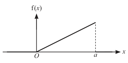
The diagram shows the graph of the probability density function $f$ of a random variable $X$ . Between $x = 0$ and $x = a$ the graph consists of a straight line through $O$ with gradient $k$ , where $k$ and $a$ are positive constants. Elsewhere $f(x) = 0$ .

It is given that the median of $X$ is $\sqrt{2}$ .

(a)

Find the value of $k$ .

2M Similar

DifficultyMedium-Easy

Worked solution

Approach

The median of a continuous random variable $X$ is the value $m$ such that the probability $P(X \le m) = 0.5$ . This corresponds to the area under the probability density function (PDF) from the lower bound to $m$ being equal to $0.5$ . Here, the lower bound is $x=0$ and the median is given as $\sqrt{2}$ . We can use the area of the triangle formed by the graph or integrate the function $f(x) = kx$ from $0$ to $\sqrt{2}$ .

Working

The function is $f(x) = kx$ for $0 \le x \le a$ . At $x = \sqrt{2}$ , the value of the function is $f(\sqrt{2}) = k\sqrt{2}$ .

Using the area of the triangle under the graph from $x=0$ to $x=\sqrt{2}$ :

\text{Area} = \frac{1}{2} \times \text{base} \times \text{height} = \frac{1}{2} \times \sqrt{2} \times k\sqrt{2} = k

Since the median is $\sqrt{2}$ , this area must be equal to $0.5$ :

k = 0.5 = \frac{1}{2}

Alternatively, using integration:

\int_0^{\sqrt{2}} kx \, \mathrm{d}x = \left[ \frac{kx^2}{2} \right]_0^{\sqrt{2}} = \frac{k(2)}{2} - 0 = k

Setting this equal to $0.5$ gives $k = \frac{1}{2}$ .

Answer

k = \frac{1}{2}

Final answer

k = 1/2

Detailed explanation

Walkthrough

The median of a continuous random variable is the value that splits the total probability (area under the PDF) into two equal halves. Since the PDF is defined for $x \ge 0$ , the area from $x=0$ to the median $x=\sqrt{2}$ must be exactly $0.5$ .

The graph from $x=0$ to $x=\sqrt{2}$ is a right-angled triangle with base $\sqrt{2}$ and height $f(\sqrt{2}) = k\sqrt{2}$ . The area of this triangle is $\frac{1}{2} \times \text{base} \times \text{height} = \frac{1}{2} \times \sqrt{2} \times k\sqrt{2} = k$ . Setting this area equal to $0.5$ immediately gives $k = 0.5$ .

Alternatively, you can integrate the function $f(x) = kx$ from $0$ to $\sqrt{2}$ :

\int_0^{\sqrt{2}} kx \, \mathrm{d}x = \left[ \frac{kx^2}{2} \right]_0^{\sqrt{2}} = \frac{k(\sqrt{2})^2}{2} = k

Equating this to $0.5$ yields the same result: $k = \frac{1}{2}$ .

Key Takeaways

The median $m$ of a continuous random variable satisfies $\int_{-\infty}^{m} f(x) \, \mathrm{d}x = 0.5$ .
The area under a PDF can be calculated using geometric formulas (like the area of a triangle) or definite integration.

Common Mistakes

Assuming the total area is calculated up to $a$ before finding $k$ . The median condition only involves the area up to $\sqrt{2}$ .
Forgetting that the area under the entire PDF must be $1$ , which is needed in part (b).

Things to Be Careful About

Ensure the limits of integration match the region for the median (from $0$ to $\sqrt{2}$ , not $0$ to $a$ ).
The gradient $k$ must be positive, and the area must be positive.

Techniques used

apply the definition of median for a continuous random variablecalculate area under a PDF using geometry or integrationsolve for unknown gradient

(b)

Find the value of $E(X)$ .

4M Similar

DifficultyMedium

Worked solution

Approach

First, we find the value of $a$ using the property that the total area under the PDF is $1$ . Once $a$ is known, we can calculate the expected value $E(X)$ using the formula $E(X) = \int_0^a x f(x) \, \mathrm{d}x$ .

Working

The total area under the PDF from $x=0$ to $x=a$ is $1$ . The shape is a triangle with base $a$ and height $f(a) = ka = \frac{1}{2}a$ (using $k=\frac{1}{2}$ from part (a)).

Using the area of the triangle:

\frac{1}{2} \times a \times \frac{1}{2}a = 1

\frac{a^2}{4} = 1 \implies a^2 = 4

Since $a$ is positive, $a = 2$ .

Alternatively, using integration:

\int_0^a \frac{1}{2}x \, \mathrm{d}x = \left[ \frac{x^2}{4} \right]_0^a = \frac{a^2}{4} = 1 \implies a = 2

Now, calculate the expected value $E(X)$ :

E(X) = \int_0^2 x \cdot f(x) \, \mathrm{d}x = \int_0^2 x \cdot \left(\frac{1}{2}x\right) \, \mathrm{d}x = \int_0^2 \frac{1}{2}x^2 \, \mathrm{d}x

Evaluate the integral:

\int_0^2 \frac{1}{2}x^2 \, \mathrm{d}x = \left[ \frac{x^3}{6} \right]_0^2 = \frac{2^3}{6} - 0 = \frac{8}{6} = \frac{4}{3}

Answer

E(X) = \frac{4}{3}

Final answer

E(X) = 4/3

Detailed explanation

Walkthrough

The total probability for any valid PDF must sum to $1$ . This means the total area under the graph from $x=0$ to $x=a$ is $1$ .

The graph is a triangle with base $a$ and height $f(a)$ . Since $f(x) = kx$ and we found $k = \frac{1}{2}$ , the height is $f(a) = \frac{1}{2}a$ .

Area = $\frac{1}{2} \times \text{base} \times \text{height} = \frac{1}{2} \times a \times \frac{1}{2}a = \frac{a^2}{4}$ .

Setting this equal to $1$ : $\frac{a^2}{4} = 1 \implies a^2 = 4 \implies a = 2$ (since $a > 0$ ).

Now we find the expected value $E(X)$ . The formula for the mean of a continuous random variable is:

E(X) = \int_{-\infty}^{\infty} x f(x) \, \mathrm{d}x

Since $f(x) = 0$ outside $[0, 2]$ , the limits are $0$ to $2$ :

E(X) = \int_0^2 x \left(\frac{1}{2}x\right) \, \mathrm{d}x = \int_0^2 \frac{1}{2}x^2 \, \mathrm{d}x

Integrating:

\left[ \frac{1}{2} \cdot \frac{x^3}{3} \right]_0^2 = \left[ \frac{x^3}{6} \right]_0^2 = \frac{8}{6} = \frac{4}{3}

Key Takeaways

The total area under a PDF is always $1$ . This is used to find unknown constants like the upper bound $a$ .
The expected value (mean) is calculated as $E(X) = \int x f(x) \, \mathrm{d}x$ .
Always multiply $x$ by the PDF $f(x)$ inside the integral for expected value.

Common Mistakes

Forgetting to multiply by $x$ when calculating $E(X)$ . The integral $\int f(x) \, \mathrm{d}x$ gives probability (which is $1$ ), not the mean.
Using the wrong limits of integration. The PDF is only non-zero between $0$ and $a=2$ .
Arithmetic errors in integrating $x^2$ (remember $\int x^2 \, \mathrm{d}x = \frac{x^3}{3}$ , not $\frac{x^2}{2}$ ).

Things to Be Careful About

Ensure you use the value of $k$ found in part (a) correctly.
The variable $a$ must be positive.
Check that the final answer for $E(X)$ is within the possible range of $X$ (i.e., $0 \le E(X) \le 2$ ). Here $\frac{4}{3} \approx 1.33$ , which is valid.

Techniques used

use total area under PDF = 1 to find upper boundset up integral for expected value E(X) = integral x f(x) dxevaluate definite integral

Mathematics 9709/65 — May/June 2025

Approach

Working

Answer

Walkthrough

Key Takeaways

Common Mistakes

Things to Be Careful About

Approach

Working

Answer

Walkthrough

Key Takeaways

Common Mistakes

Things to Be Careful About

Approach

Working

Answer

Walkthrough

Key Takeaways

Common Mistakes

Things to Be Careful About

Approach

Working

Answer

Walkthrough

Key Takeaways

Common Mistakes

Things to Be Careful About

Approach

Working

Answer

Walkthrough

Key Takeaways

Common Mistakes

Things to Be Careful About

Approach

Working

Answer

Walkthrough

Key Takeaways

Common Mistakes

Things to Be Careful About

Approach

Working

Answer

Walkthrough

Key Takeaways

Common Mistakes

Things to Be Careful About

Approach

Working

Answer

Walkthrough

Key Takeaways

Common Mistakes

Things to Be Careful About

Approach

Working

Answer

Walkthrough

Key Takeaways

Common Mistakes

Things to Be Careful About

Approach

Working

Answer

Walkthrough

Key Takeaways

Common Mistakes

Things to Be Careful About

Approach

Working

Answer

Walkthrough

Key Takeaways

Common Mistakes

Things to Be Careful About

Approach

Working