The random variable $X$ has the distribution $Po(1.5)$. (a) Find $P(X \geq 3)$. (b) Find the probability that the sum of three independent values of $X$ is between 3 and 5 inclusive. (c) The sum of a large number, $n$, of values of $X$ is denoted by $T$. Using a suitable approximation, it was found that $P(T > 330) = 0.0391$, correct to 3 significant figures. Find the value of $n$.

(a) 0.191 · (b) 0.529 · (c) n = 200

(a) The diagram shows the graph of the probability density function, $f$, of a random variable $X$. The graph is a straight line from $(0, a)$ to $(2, b)$, where $a$ and $b$ are positive constants. Elsewhere, $f(x) = 0$. (i) Show that $b = 1 - a$. (ii) Given that $E(X) = 1.2$, find the value of $a$. (b) A random variable $T$ has probability density function given by $$ g(t) = \begin{cases} \frac{1}{2}\cos t & -\frac{1}{2}\pi \leq t \leq \frac{1}{2}\pi, \\ 0 &…

(a)(i) b = 1 - a · (a)(ii) a = 0.2 · (b) c = π/6

9709/62 Feb/Mar 2025 — Mathematics Solved Past Paper

Q15MMedium-EasyLinear Combinations of Random Variables

The random variables $X$ and $Y$ have the independent distributions $N(44, 16)$ and $N(30, 9)$ respectively.

Find $P(X - Y < 15)$ .

DifficultyMedium-Easy

Worked solution

Approach

Since $X$ and $Y$ are independent normal random variables, their difference $X - Y$ is also normal. Let $W = X - Y$ . Find the mean and variance of $W$ , standardise the value $15$ , and then use the standard normal distribution table.

Working

Let $W = X - Y$ . Because $X$ and $Y$ are independent and normal, $W$ is normal.

E(W) = E(X) - E(Y) = 44 - 30 = 14

\operatorname{Var}(W) = \operatorname{Var}(X) + \operatorname{Var}(Y) = 16 + 9 = 25

So $W \sim N(14, 25)$ , and the standard deviation is $\sqrt{25} = 5$ .

Standardise:

P(X - Y < 15) = P\left(Z < \frac{15 - 14}{5}\right) = P(Z < 0.2)

From the standard normal table:

P(Z < 0.2) = \Phi(0.2) = 0.5793

Answer

P(X - Y < 15) = 0.579 \quad (3 \text{ sf})

Final answer

0.579

Detailed explanation

Walkthrough

We are given two independent normal random variables: $X \sim N(44, 16)$ and $Y \sim N(30, 9)$ . The first number in each is the mean and the second is the variance. We need $P(X - Y < 15)$ .

Because $X$ and $Y$ are independent and normal, the linear combination $W = X - Y$ is also normal. For a difference of two variables, the mean is the difference of the means, and the variance is the sum of the variances:

E(W) = 44 - 30 = 14, \quad \operatorname{Var}(W) = 16 + 9 = 25

Thus $W \sim N(14, 25)$ , so its standard deviation is $\sqrt{25} = 5$ .

To find $P(W < 15)$ , standardise:

z = \frac{15 - 14}{5} = 0.2

Then $P(W < 15) = P(Z < 0.2) = \Phi(0.2) = 0.5793$ , which is $0.579$ to 3 significant figures.

Key Takeaways

A linear combination of independent normal random variables is normal.
For $E(X - Y)$ , the mean is $E(X) - E(Y)$ .
For independent variables, variances add: $\operatorname{Var}(X - Y) = \operatorname{Var}(X) + \operatorname{Var}(Y)$ .
To find a probability, standardise using $z = \frac{x - \mu}{\sigma}$ and then use the standard normal table.

Common Mistakes

Subtracting the variances instead of adding them. Even though we are subtracting $Y$ , independence means the variances add.
Using the variance $25$ as the standard deviation. The standard deviation is $\sqrt{25} = 5$ .
Forgetting to standardise before using the normal table.
Using the wrong tail: since the inequality is $<$ , we need the lower-tail probability $\Phi(0.2)$ .
Rounding too early: keep $0.5793$ and round to $0.579$ at the end.

Things to Be Careful About

The variance of $X - Y$ is $16 + 9 = 25$ , not $16 - 9$ .
The standard deviation is $5$ , so the standardised value is $\frac{15 - 14}{5} = 0.2$ .
No continuity correction is needed because the normal distribution is continuous.
The mark scheme allows standardisation with the student's own mean and variance values, but the final probability must be consistent with those values.

Techniques used

form a linear combination of independent normal variablescompute the mean and variance of the differencestandardise a normal variableread a cumulative probability from the standard normal table

Approach

Use the sample summaries to estimate the population mean with $\hat{\mu} = \frac{\sum t}{n}$ . For the variance, use the unbiased estimator

s^2 = \frac{1}{n-1}\left(\sum t^2 - \frac{(\sum t)^2}{n}\right)

Working

Calculate the estimate of $E(T)$ :

\hat{\mu} = \frac{3678}{60} = 61.3

Now calculate the unbiased estimate of the variance:

s^2 = \frac{1}{59}\left(226313.36 - \frac{3678^2}{60}\right)

First,

\frac{3678^2}{60} = \frac{13527684}{60} = 225461.4

So

s^2 = \frac{1}{59}(226313.36 - 225461.4) = \frac{851.96}{59}

s^2 = 14.44

Answer

$\hat{\mu} = 61.3$ and $s^2 = 14.44$ , so the unbiased estimate of $\mathrm{Var}(T)$ is $14.44$ as required.

Final answer

hat(mu) = 61.3; s^2 = 14.44

Detailed explanation

Walkthrough

The question gives summary data from a random sample: $n = 60$ , $\sum t = 3678$ and $\sum t^2 = 226313.36$ .

We first estimate the population mean time $E(T)$ by the sample mean:

\hat{\mu} = \bar t = \frac{\sum t}{n}

For the variance, the sample variance with divisor $n-1$ is an unbiased estimator of the population variance. A convenient computational form is

s^2 = \frac{1}{n-1}\left(\sum t^2 - \frac{(\sum t)^2}{n}\right)

Substitute $\sum t^2 = 226313.36$ , $\sum t = 3678$ and $n = 60$ .

The bracket simplifies as

226313.36 - \frac{3678^2}{60} = 226313.36 - 225461.4 = 851.96

Then

s^2 = \frac{851.96}{59} = 14.44

This matches the stated value, so the computation is consistent.

Key Takeaways

An unbiased estimate of the population mean is the sample mean.
To estimate population variance from a sample, use divisor $n-1$ .
The identity $\sum (t - \bar t)^2 = \sum t^2 - \frac{(\sum t)^2}{n}$ is useful.

Common Mistakes

Using $n$ instead of $n-1$ in the denominator.
Arithmetic errors when dividing $3678^2$ by $60$ .
Treating $\hat{\mu}$ as the population mean rather than an estimate.

Things to Be Careful About

Keep enough decimal places while calculating; the final value should be exactly $14.44$ .
Since the value $14.44$ is given in the question, the working must show the correct expression and clearly lead to that value.

Techniques used

calculate the sample meanapply the unbiased variance formula with divisor n-1substitute sample summary statistics

(b)

In the past, the population mean time was 62.4 seconds.

Test at the 2% significance level whether the population mean time for this year is less than 62.4 seconds.

5M Similar

DifficultyMedium

Worked solution

Approach

This is a one-tailed hypothesis test for a population mean, using a large sample so the sample mean is approximately normal. State the null and alternative hypotheses, standardise the sample mean, then compare with the 2% critical value.

Working

Let $\mu$ be the population mean time this year.

H_0: \mu = 62.4 \qquad H_1: \mu < 62.4

Use the test statistic

z = \frac{\bar t - 62.4}{\sqrt{\frac{s^2}{n}}}

with $\bar t = 61.3$ , $s^2 = 14.44$ and $n = 60$ :

z = \frac{61.3 - 62.4}{\sqrt{\frac{14.44}{60}}}

z = \frac{-1.1}{\sqrt{0.240666\ldots}} = -2.242

The critical value for a 2% one-tailed test in the lower tail is

z^* = -2.054

Compare:

-2.242 < -2.054

Equivalently, the $p$ -value is $P(Z < -2.242) = 0.0124 < 0.02$ , so the result is significant.

Reject $H_0$ .

Answer

There is sufficient evidence at the 2% significance level to suggest that the population mean time this year is less than 62.4 seconds, so the mean time has decreased.

Final answer

Reject H0; there is sufficient evidence that the population mean time is less than 62.4 seconds.

Detailed explanation

Walkthrough

This is a hypothesis test about a population mean. The historical value is 62.4 seconds, and we want to know whether this year's mean is lower. Because the sample size is 60, we use the normal distribution for the sample mean.

Start by writing the hypotheses. Use the population mean $\mu$ and choose the alternative according to the claim:

H_0: \mu = 62.4, \quad H_1: \mu < 62.4

The significance level is 2% and the alternative is one-sided (less than), so the critical region is the lower 2% tail of the standard normal distribution.

Use the sample mean $\bar t = 61.3$ and the unbiased variance estimate $s^2 = 14.44$ from part (a). The standard error of the sample mean is $\sqrt{s^2/n}$ , so the test statistic is

z = \frac{61.3 - 62.4}{\sqrt{14.44/60}} = -2.242

Compare this with the critical value for a 2% one-tail test, $-2.054$ . Since $-2.242$ is further into the tail than $-2.054$ , the result is significant.

Equivalently, the $p$ -value is $0.0124$ , which is less than 0.02.

Thus we reject $H_0$ and conclude in context that there is sufficient evidence that the population mean time this year is less than 62.4 seconds.

Key Takeaways

Always state hypotheses in terms of the population mean $\mu$ .
For a one-tailed test, use the one-tailed critical value (here the 2% tail on the lower side).
Standardise the sample mean using the sample variance divided by the sample size.
Reject or do not reject $H_0$ based on whether the test statistic falls in the critical region, or equivalently whether the $p$ -value is less than the significance level.

Common Mistakes

Using a two-tailed test and comparing with 2.326 instead of 2.054.
Writing that the mean time has decreased as a definite statement; the correct conclusion is that there is evidence that it has decreased.
Forgetting the $\sqrt{60}$ in the standard error.
Not giving the conclusion in context.

Things to Be Careful About

The test statistic is negative here because the sample mean is below the hypothesised mean; compare it with the negative critical value.
The variance used is the estimate from part (a), not a known population variance.
No continuity correction is needed for this test.
Use at least 3 significant figures when stating the test statistic.

Techniques used

state null and alternative hypothesesstandardise the sample meancompare the test statistic with the critical valuedraw a conclusion in context

(c)

State, with a reason, whether it was necessary to use the Central Limit Theorem in your answer to part (b).

1M Similar

Q3Medium-HardThe Poisson DistributionLinear Combinations of Random Variables

The random variable $X$ has the distribution $Po(1.5)$ .

(a)

Find $P(X \geq 3)$ .

2M Similar

DifficultyMedium-Easy

Worked solution

Approach

Since $X \sim Po(1.5)$ , we use the complement rule:

P(X \geq 3) = 1 - P(X \leq 2)

Then calculate $P(X \leq 2)$ using the Poisson formula.

Working

For $X \sim Po(\lambda)$ ,

P(X = x) = e^{-\lambda} \frac{\lambda^x}{x!}

With $\lambda = 1.5$ :

P(X \leq 2) = e^{-1.5}\left(1 + 1.5 + \frac{1.5^2}{2}\right)

= e^{-1.5}(1 + 1.5 + 1.125)

= 0.22313 + 0.334695 + 0.25102 = 0.808845

Therefore

P(X \geq 3) = 1 - 0.808845 = 0.191155

Answer

P(X \geq 3) = 0.191

Final answer

0.191

Detailed explanation

Walkthrough

We want the probability that a Poisson random variable with mean 1.5 takes a value of 3 or more. Because the Poisson distribution has no upper limit, it is easier to calculate the complement: the probability that $X$ is 0, 1 or 2, and subtract this from 1.

For each value $x$ , the Poisson formula gives $P(X=x)=e^{-1.5}\frac{1.5^x}{x!}$ . Adding the three probabilities gives $P(X \leq 2)$ . The mark scheme awards the method mark for setting up this sum and the accuracy mark for the final numerical value.

Key Takeaways

This question tests the ability to use the Poisson probability formula and to choose the complement when calculating an upper-tail probability. It also shows the importance of including all terms from 0 up to the boundary value.

Common Mistakes

Forgetting to include $P(X=0)$ when calculating $P(X \leq 2)$ .
Using $P(X \geq 3) = 1 - P(X = 2)$ instead of $1 - P(X \leq 2)$ .
Rounding intermediate values too early, which can change the final 3-significant-figure answer.

Things to Be Careful About

The mark scheme allows one end error, but an unsupported correct answer scores only B1 rather than full marks, so all working should be shown. Use $\lambda = 1.5$ and keep enough decimal places until the final subtraction.

Techniques used

use the complement rulecalculate Poisson probabilities for x = 0, 1, 2subtract the cumulative probability from 1

(b)

Find the probability that the sum of three independent values of $X$ is between 3 and 5 inclusive.

3M Similar

DifficultyMedium

Worked solution

Approach

The sum of independent Poisson random variables is also Poisson, with parameter equal to the sum of the parameters. Let $S = X_1 + X_2 + X_3$ . Then $S \sim Po(4.5)$ . We need $P(3 \leq S \leq 5)$ , so we add $P(S=3)$ , $P(S=4)$ and $P(S=5)$ .

Working

Since $X_i \sim Po(1.5)$ independently,

S = X_1 + X_2 + X_3 \sim Po(4.5)

Using $P(S=s)=e^{-4.5}\frac{4.5^s}{s!}$ :

P(3 \leq S \leq 5) = e^{-4.5}\left(\frac{4.5^3}{3!} + \frac{4.5^4}{4!} + \frac{4.5^5}{5!}\right)

= e^{-4.5}(15.1875 + 17.0859 + 15.3773)

= 0.1687 + 0.1898 + 0.1708

= 0.5293

Answer

P(3 \leq S \leq 5) = 0.529

Final answer

0.529

Detailed explanation

Walkthrough

The sum of independent Poisson random variables is again Poisson, with parameter equal to the sum of the individual parameters. Here we have three independent values of $X$ , each with parameter 1.5, so their sum $S$ has parameter $4.5$ .

Because the question asks for the probability that the sum is between 3 and 5 inclusive, we need $P(S=3)+P(S=4)+P(S=5)$ . Each probability is found from the Poisson formula with $\lambda = 4.5$ . The method mark is awarded for setting up this sum, and the accuracy mark for evaluating it correctly.

Key Takeaways

This question combines the Poisson sum property with the calculation of a range probability. It is important to recognise when a sum of independent Poisson variables can be treated as a single Poisson variable.

Common Mistakes

Using $\lambda = 1.5$ instead of $\lambda = 4.5$ for the sum.
Forgetting that "between 3 and 5 inclusive" includes 3, 4 and 5.
Omitting one of the three probabilities or using the wrong factorial in the denominator.

Things to Be Careful About

The mark scheme notes that an unsupported correct answer scores only B1 B1, so show the full summation. It also allows one end error, but the final answer must be correct to 3 significant figures.

Techniques used

add the parameters of independent Poisson variableswrite the Poisson probability for a range of valuesevaluate and sum the required probabilities

(c)

The sum of a large number, $n$ , of values of $X$ is denoted by $T$ . Using a suitable approximation, it was found that $P(T > 330) = 0.0391$ , correct to 3 significant figures.

Find the value of $n$ .

5M Similar

DifficultyMedium-Hard

Worked solution

Approach

Each value of $X$ has mean and variance $1.5$ . For $n$ independent values, $T \sim Po(1.5n)$ , so for large $n$ we approximate $T$ by a normal distribution with mean $1.5n$ and variance $1.5n$ . Apply a continuity correction to the boundary $330$ , standardise, and use the given upper-tail probability to find the corresponding $z$ -value. Then solve the resulting equation for $n$ .

Working

Since $T$ is the sum of $n$ independent $Po(1.5)$ variables,

T \sim Po(1.5n)

For large $n$ , use the normal approximation:

T \approx N(1.5n,\, 1.5n)

With continuity correction, $P(T > 330)$ becomes $P(T \geq 331)$ , so standardise using $330.5$ :

P\left(Z > \frac{330.5 - 1.5n}{\sqrt{1.5n}}\right) = 0.0391

The upper-tail probability $0.0391$ corresponds to

z = \Phi^{-1}(1 - 0.0391) = \Phi^{-1}(0.9609) = 1.761

Therefore

\frac{330.5 - 1.5n}{\sqrt{1.5n}} = 1.761

Let $u = \sqrt{n}$ . Then $\sqrt{1.5n} = \sqrt{1.5}\,u$ and $1.5n = 1.5u^2$ , so

330.5 - 1.5u^2 = 1.761\sqrt{1.5}\,u

1.5u^2 + 2.1568u - 330.5 = 0

Solving the quadratic in $u$ :

u = \frac{-2.1568 + \sqrt{2.1568^2 + 4(1.5)(330.5)}}{2(1.5)}

u = 14.14 \quad (\text{reject the negative root})

Thus

\sqrt{n} = 14.14 \Rightarrow n = 200

Answer

n = 200

Final answer

n = 200

Detailed explanation

Walkthrough

We are told that $T$ is the sum of a large number $n$ of independent values of $X$ , where $X \sim Po(1.5)$ . Since the sum of independent Poisson variables is Poisson, $T \sim Po(1.5n)$ . For large $n$ , the Poisson distribution can be approximated by a normal distribution with the same mean and variance, so $T \approx N(1.5n, 1.5n)$ .

The event $T > 330$ is discrete. With the continuity correction, we treat it as $T \geq 331$ , so the boundary used for standardising is $330.5$ . The given probability $0.0391$ is the upper tail, so we find the corresponding $z$ -value from the inverse normal distribution: $\Phi^{-1}(0.9609) = 1.761$ .

We then standardise $330.5$ using the mean $1.5n$ and standard deviation $\sqrt{1.5n}$ , set the result equal to $1.761$ , and solve for $n$ . Substituting $u = \sqrt{n}$ turns the equation into a quadratic in $u$ . The positive root gives $\sqrt{n} = 14.14$ , so $n = 200$ .

Key Takeaways

This question tests the normal approximation to the Poisson distribution, the continuity correction, and the use of inverse normal values. It also requires forming and solving a quadratic equation in a transformed variable such as $\sqrt{n}$ .

Common Mistakes

Omitting the continuity correction and using 330 instead of 330.5.
Using the variance $1.5n$ as the standard deviation instead of $\sqrt{1.5n}$ .
Forgetting to reject the negative root when solving the quadratic.
Rounding the $z$ -value or intermediate values too early.

Things to Be Careful About

The mark scheme accepts the normal approximation even if the continuity correction is omitted for the method marks, but the final accuracy mark depends on using $330.5$ . Keep enough precision in $z = 1.761$ and in the quadratic coefficients to obtain $n = 200$ .

Techniques used

approximate a Poisson distribution by a normal distributionapply a continuity correctionuse the inverse normal distribution to find the standardised valueform and solve a quadratic equation in sqrt(n)

Q4MediumContinuous Random Variables

(a)

Fig. 4.1

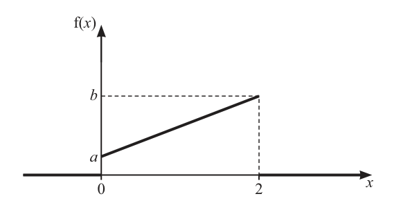
The diagram shows the graph of the probability density function, $f$ , of a random variable $X$ . The graph is a straight line from $(0, a)$ to $(2, b)$ , where $a$ and $b$ are positive constants. Elsewhere, $f(x) = 0$ .

7M

(i)

Show that $b = 1 - a$ .

2M Similar

(ii)

Given that $E(X) = 1.2$ , find the value of $a$ .

5M Similar

DifficultyMedium

Worked solution

Approach

Find the equation of the line in terms of $a$ (using $b = 1 - a$ from the previous part), then evaluate $E(X) = \int_0^2 x\,f(x)\,dx$ and solve the resulting equation for $a$ .

Working

The line passes through $(0, a)$ and $(2, 1 - a)$ , so its slope is

\frac{(1 - a) - a}{2} = \frac{1 - 2a}{2}.

Hence

f(x) = a + \frac{1 - 2a}{2}\,x.

The expectation is

E(X) = \int_0^2 x\,f(x)\,dx = \int_0^2 \left(ax + \frac{1-2a}{2}\,x^2\right)dx.

Integrating:

= \left[\frac{ax^2}{2} + \frac{(1 - 2a)x^3}{6}\right]_0^2.

Substituting the limits:

= 2a + \frac{4(1 - 2a)}{3} = \frac{6a + 4 - 8a}{3} = \frac{4 - 2a}{3}.

Setting $E(X) = 1.2$ :

\frac{4 - 2a}{3} = 1.2

4 - 2a = 3.6

2a = 0.4 \quad \Rightarrow \quad a = 0.2.

Answer

a = 0.2

Final answer

a = 0.2

Detailed explanation

Walkthrough

With $b = 1 - a$ established, the line joining $(0,a)$ to $(2, 1-a)$ has gradient $\frac{(1-a) - a}{2} = \frac{1-2a}{2}$ , giving the linear PDF $f(x) = a + \frac{1-2a}{2}x$ . The expectation of a continuous random variable is $E(X) = \int x\,f(x)\,dx$ , so we need to compute $\int_0^2 x\left(a + \frac{1-2a}{2}x\right)dx$ . Expanding gives $ax + \frac{1-2a}{2}x^2$ , and integrating term-by-term yields $\frac{ax^2}{2} + \frac{(1-2a)x^3}{6}$ . Substituting the limits $0$ and $2$ produces $2a + \frac{4(1-2a)}{3} = \frac{4 - 2a}{3}$ . Setting this equal to the given $E(X) = 1.2$ gives a simple linear equation in $a$ whose solution is $a = 0.2$ .

Key Takeaways

For a linear PDF, $E(X) = \int x \cdot f(x)\,dx$ , which is the first moment of the density.
The gradient of a line through two known points gives the linear function directly.
After integration, expectations in such problems reduce to straightforward linear equations.

Common Mistakes

Forgetting to multiply by $x$ inside the integral — computing $\int f(x)\,dx$ instead of $\int x\,f(x)\,dx$ .
Sign errors when computing the gradient (subtracting in the wrong order).
Mis-substituting the upper limit; the cube of $2$ is $8$ , not $4$ .

Things to Be Careful About

The mark scheme's B1 step allows this line equation to have been seen in part (a)(i) — keep the form consistent.
Equate to $1.2$ exactly; $1.2 = \frac{6}{5}$ if you prefer working in fractions.

Techniques used

write equation of line in terms of aset up integral for E(X)integrate x times the PDFsubstitute limits and solve linear equation

(b)

A random variable $T$ has probability density function given by

g(t) = \begin{cases} \frac{1}{2}\cos t & -\frac{1}{2}\pi \leq t \leq \frac{1}{2}\pi, \\ 0 & \text{otherwise.} \end{cases}

Find the value of $c$ such that $P(-c < t < c) = \frac{1}{2}$ .

4M Similar

DifficultyMedium-Easy

Worked solution

Approach

Express $P(-c < t < c)$ as a definite integral of the given PDF, evaluate it using the fact that $\cos t$ is even, and solve the resulting trigonometric equation for $c$ .

Working

P(-c < t < c) = \int_{-c}^{c} \frac{1}{2}\cos t\,dt = \frac{1}{2}\bigl[\sin t\bigr]_{-c}^{c} = \frac{1}{2}(\sin c - \sin(-c)) = \frac{1}{2}(2\sin c) = \sin c.

Setting this equal to $\frac{1}{2}$ :

\sin c = \frac{1}{2}.

Since $0 \leq c \leq \frac{\pi}{2}$ (from the support of the PDF):

c = \frac{\pi}{6}.

Answer

c = \frac{\pi}{6}

Final answer

c = π/6

Detailed explanation

Walkthrough

For a continuous random variable, a probability is the integral of the PDF over the relevant interval. The PDF here is $\frac{1}{2}\cos t$ on $\left[-\frac{\pi}{2}, \frac{\pi}{2}\right]$ , so $P(-c < t < c) = \int_{-c}^{c} \frac{1}{2}\cos t\,dt$ . Because $\cos t$ is an even function, we can write $\int_{-c}^{c}\cos t\,dt = 2\int_0^c \cos t\,dt = 2\sin c$ , or more directly $\frac{1}{2}[\sin c - \sin(-c)] = \frac{1}{2}(2\sin c) = \sin c$ . Setting $\sin c = \frac{1}{2}$ and taking $c$ in $[0, \pi/2]$ (the only relevant range from the PDF's support) gives $c = \pi/6$ .

Key Takeaways

A probability for a continuous random variable is the area under the PDF between two limits.
$\cos t$ is even, so integrals symmetric about $0$ can be written as twice the integral from $0$ .
When inverting $\sin c = k$ , choose the principal value within the support of the PDF.

Common Mistakes

Forgetting the factor of $\frac{1}{2}$ in the PDF and solving $\sin c = 1$ instead.
Choosing the wrong branch of the inverse sine, e.g. $c = \frac{5\pi}{6}$ , which is outside the support of $T$ .
Using degrees instead of radians (the PDF is defined in radians).

Things to Be Careful About

The support of the PDF is $\left[-\frac{\pi}{2}, \frac{\pi}{2}\right]$ , so the valid range for $c$ is $\left[0, \frac{\pi}{2}\right]$ .

Techniques used

set up definite integral for probabilityintegrate cosineapply odd-function symmetryinvert sine function

Q5Medium-EasyHypothesis Tests

Amir believes that 20% of the students at his college are left-handed. His friend believes that the true proportion, $p$ , is less than 20%. Amir plans to use the binomial distribution to test the null hypothesis, $H_0: p = 0.2$ , against the alternative hypothesis, $H_1: p < 0.2$ .

He decides to choose 35 students at random. If 3 or fewer of these students are left-handed, Amir will reject his belief.

(a)

Find the significance level of the test.

3M Similar

DifficultyMedium-Easy

Worked solution

Approach

Under $H_0$ , the number of left-handed students in the sample is $X \sim B(35, 0.2)$ . Amir rejects $H_0$ when $X \le 3$ . The significance level is the probability of rejecting $H_0$ when $H_0$ is true:

P(X \le 3)

Working

Using the binomial distribution with $n = 35$ and $p = 0.2$ :

\begin{aligned} P(X \le 3) &= 0.8^{35} + \binom{35}{1}(0.2)(0.8^{34}) + \binom{35}{2}(0.2)^2(0.8^{33}) + \binom{35}{3}(0.2)^3(0.8^{32}) \\ &= 0.0004056 + 0.0035494 + 0.015085 + 0.0414838 \\ &= 0.0605 \end{aligned}

The four terms are the probabilities that exactly 0, 1, 2 and 3 students are left-handed.

Answer

The significance level is $0.0605$ , or 6.05%.

Final answer

0.0605 (6.05%)

Detailed explanation

Walkthrough

Under the null hypothesis $H_0: p = 0.2$ , the number $X$ of left-handed students among the 35 chosen has a binomial distribution $B(35, 0.2)$ . Amir's decision rule is to reject $H_0$ if $X \le 3$ . The significance level of the test is the probability of rejecting $H_0$ when $H_0$ is actually true, so we need $P(X \le 3)$ using $p = 0.2$ . This is the sum of the probabilities of exactly 0, 1, 2 and 3 left-handed students. Each term has the form $\binom{35}{r}(0.2)^r(0.8)^{35-r}$ . Adding the four calculated probabilities gives $0.0605$ , so the test has significance level 6.05%.

Key Takeaways

A significance level is the probability of rejecting a true null hypothesis. For a binomial test with rejection region $X \le 3$ , it is the lower-tail binomial probability under $H_0$ . The calculation requires summing all probabilities in the rejection region.

Common Mistakes

Omitting the $X = 0$ term and starting from $X = 1$ ; the rejection region is $X \le 3$ , so $X = 0$ must be included.
Using $p = 0.3$ or the complement tail $P(X > 3)$ instead of $P(X \le 3)$ .
Giving an unsupported answer of 6.05% without showing the binomial calculation; the method mark may not be awarded.
Rounding each term to too few decimal places before adding, which can change the final answer.

Things to Be Careful About

The significance level must be calculated under $H_0: p = 0.2$ , not under the sample result. The final value $0.0605$ corresponds to 6.05%. The mark scheme accepts 6.05%, 6.1% or 6%, and also accepts values in the range 6.05% to 14.3% if a different valid method is used, but the standard binomial calculation gives 0.0605.

Techniques used

identify the binomial model under the null hypothesiswrite the cumulative binomial probability for the rejection regionevaluate the four binomial probability terms to obtain the significance level

(b)

State the probability of a Type I error.

1M Similar

(c)

It is now given that the true value of $p$ is 0.05.

Find the probability of a Type II error.

3M Similar

DifficultyMedium-Easy

Worked solution

Approach

A Type II error occurs when $H_0$ is not rejected even though $H_1$ is true. Now the true proportion is $p = 0.05$ , so $X \sim B(35, 0.05)$ . Since Amir rejects when $X \le 3$ , failing to reject means $X > 3$ . Therefore:

P(\text{Type II error}) = P(X > 3) = 1 - P(X \le 3)

Working

Under $p = 0.05$ :

\begin{aligned} P(X \le 3) &= 0.95^{35} + \binom{35}{1}(0.05)(0.95^{34}) + \binom{35}{2}(0.05)^2(0.95^{33}) + \binom{35}{3}(0.05)^3(0.95^{32}) \\ &= 0.1661 + 0.3059 + 0.2737 + 0.1585 \\ &= 0.9042 \end{aligned}

Therefore:

P(X > 3) = 1 - 0.9042 = 0.0958

Answer

The probability of a Type II error is $0.0958$ .

Final answer

0.0958

Detailed explanation

Walkthrough

Now we use the true value $p = 0.05$ , so $X$ has distribution $B(35, 0.05)$ . A Type II error occurs when the null hypothesis is false but Amir fails to reject it. Amir rejects when $X \le 3$ , so failing to reject means $X > 3$ . We first compute $P(X \le 3)$ by adding the probabilities of exactly 0, 1, 2 and 3 left-handed students, using $p = 0.05$ . The sum is $0.9042$ . The probability of the complementary event, $X > 3$ , is $1 - 0.9042 = 0.0958$ .

Key Takeaways

The probability of a Type II error is calculated under the true alternative proportion, not under the null hypothesis. It is the probability that the sample result falls outside the rejection region when $H_1$ is true. Here the rejection region is $X \le 3$ , so the fail-to-reject region is $X \ge 4$ .

Common Mistakes

Using $p = 0.2$ again; a Type II error must be calculated under the true value $p = 0.05$ .
Computing $P(X \le 3)$ and giving 0.9042 directly instead of taking the complement $1 - 0.9042$ .
Forgetting to include all terms $X = 0$ to $X = 3$ .
Giving an unsupported final answer of 0.0958; the working method should be shown to earn the method mark.

Things to Be Careful About

The mark scheme awards a mark for using $B(35, 0.05)$ , a method mark for the correct cumulative sum and complement, and the final accuracy mark for $0.0958$ . Depending on rounding, 0.0957 is also accepted. Give the final probability to 3 significant figures.

Techniques used

identify the binomial model under the true alternative proportioncalculate the cumulative binomial probability P(X <= 3) for B(35, 0.05)take the complement to find the probability of failing to reject a false null hypothesis

Q6MediumSampling and Estimation

Nikki is investigating the views of students at her school about the school sports facilities. She plans to give a survey to a sample of students.

Nikki's friend says, "This survey is about sports facilities, so you should choose a sample of students from the school sports teams."

(a)

State, with a reason, whether you agree with Nikki's friend.

1M Similar

(b)

Nikki chooses an appropriate random sample of 60 students. She finds that 45 of these students think that the sports facilities are good.

Calculate an approximate 95% confidence interval for the proportion of students who think that the sports facilities are good.

3M Similar

DifficultyMedium-Easy

Worked solution

Approach

Use the normal approximation for a confidence interval for a population proportion, $\hat{p} \pm z\sqrt{\frac{\hat{p}(1-\hat{p})}{n}}$ , with $z = 1.96$ for a 95% confidence level.

Working

The sample proportion is

\hat{p} = \frac{45}{60} = 0.75

The standard error is

\sqrt{\frac{\hat{p}(1-\hat{p})}{n}} = \sqrt{\frac{0.75 \times 0.25}{60}} = \sqrt{0.003125} = 0.0559

The margin of error is

1.96 \times 0.0559 = 0.1096

So the confidence interval is

0.75 \pm 0.1096 = (0.6404, 0.8596)

Answer

0.640 \text{ to } 0.860 \text{ (3 sf)}

Final answer

0.640 to 0.860 (or 0.64 to 0.86)

Detailed explanation

Walkthrough

We are given a sample of 60 students and 45 of them think the facilities are good. The sample proportion is $\hat{p} = 45/60 = 0.75$ . For a 95% confidence interval we use $z = 1.96$ . The standard error of the proportion is $\sqrt{\hat{p}(1-\hat{p})/n}$ . After calculating the standard error, we multiply by $z$ to get the margin of error and then add and subtract it from $\hat{p}$ to obtain the interval.

Key Takeaways

The confidence interval for a proportion is $\hat{p} \pm z\sqrt{\frac{\hat{p}(1-\hat{p})}{n}}$ .
For a 95% confidence level, $z = 1.96$ .
The interval must be given as a range, not a single value.

Common Mistakes

Using $\hat{p}$ but forgetting $1-\hat{p}$ .
Using the wrong $z$ -value, such as 1.645 or 2.576.
Not rounding to 3 significant figures.
Giving only one endpoint instead of the full interval.

Things to Be Careful About

The mark scheme awards the first mark for the formula, the second for $z = 1.96$ , and the third for the correct interval.
The correct interval is $0.640$ to $0.860$ (3 sf).
Write the answer as an interval, not as a single number.

Techniques used

compute the sample proportioncompute the standard error of a proportionconstruct a confidence interval using the normal approximation

(c)

For a different investigation, Nikki uses another large random sample to calculate a 99% confidence interval and an $x$ % confidence interval.

The width of the 99% confidence interval is double the width of the $x$ % confidence interval.

Calculate the value of $x$ .

4M Similar

DifficultyMedium

Worked solution

Approach

For a confidence interval, the width is proportional to the $z$ -value. Find the $z$ -value for a 99% interval, halve it for the $x\%$ interval, then convert that $z$ -value back to the central probability.

Working

For a 99% confidence interval, the upper tail probability is $0.005$ , so

z_{99} = \Phi^{-1}(0.995) = 2.576

Since the width of the 99% interval is double the width of the $x\%$ interval,

z_x = \frac{z_{99}}{2} = \frac{2.576}{2} = 1.288

Now

\Phi(1.288) = 0.9012

The central probability for the $x\%$ interval is

2\Phi(z_x) - 1 = 2(0.9012) - 1 = 0.8024

Therefore

x = 100 \times 0.8024 = 80.24

So $x \approx 80.2$ (or $80$ ).

Answer

x = 80.2\% \text{ (or } 80\%)

Final answer

x = 80.2% (or 80%)

Detailed explanation

Walkthrough

The width of a confidence interval is proportional to the $z$ -value because the margin of error is $z \times$ standard error. For a 99% confidence interval, the upper tail probability is $0.005$ , so $z_{99} = \Phi^{-1}(0.995) = 2.576$ . Since the 99% interval is twice as wide as the $x\%$ interval, the $z$ -value for the $x\%$ interval is half of $2.576$ , which is $1.288$ . Then $\Phi(1.288) = 0.9012$ . The central probability for a confidence level is $2\Phi(z) - 1$ , so it is $2(0.9012) - 1 = 0.8024$ . Multiplying by 100 gives $x = 80.24$ , so $x \approx 80.2$ .

Key Takeaways

Width is proportional to the $z$ -value, not to the confidence level directly.
To find the $z$ -value for a confidence level, use the inverse normal function.
To convert a $z$ -value back to a confidence level, use $2\Phi(z) - 1$ .

Common Mistakes

Using $\Phi(0.995)$ instead of $\Phi^{-1}(0.995)$ .
Not halving the $z$ -value.
Forgetting to convert the central probability to a percentage.
Using $z = 1.96$ for a 99% confidence level.

Things to Be Careful About

The mark scheme allows $\Phi^{-1}(0.99)$ as a possible starting point.
The final value can be $80.2$ to $80.3$ or $80$ .
The answer must be expressed as a percentage.

Techniques used

relate confidence interval width to the z-valueuse the inverse normal function to find a z-valuehalve the z-valueconvert a z-value back to a central probability

Mathematics 9709/62 — February/March 2025

Approach

Working

Answer

Walkthrough

Key Takeaways

Common Mistakes

Things to Be Careful About

Approach

Working

Answer

Walkthrough

Key Takeaways

Common Mistakes

Things to Be Careful About

Approach

Working

Answer

Walkthrough

Key Takeaways

Common Mistakes

Things to Be Careful About

Approach

Working

Answer

Walkthrough

Key Takeaways

Common Mistakes

Things to Be Careful About

Approach

Working

Answer

Walkthrough

Key Takeaways

Common Mistakes

Things to Be Careful About

Approach

Working

Answer

Walkthrough

Key Takeaways

Common Mistakes

Things to Be Careful About

Approach

Working

Answer

Walkthrough

Key Takeaways

Common Mistakes

Things to Be Careful About

Approach

Working

Answer

Walkthrough

Key Takeaways

Common Mistakes

Things to Be Careful About

Approach

Working

Answer

Walkthrough

Key Takeaways

Common Mistakes

Things to Be Careful About

Approach

Working

Answer

Walkthrough

Key Takeaways

Common Mistakes

Things to Be Careful About

Approach

Working

Answer

Walkthrough

Key Takeaways

Common Mistakes

Things to Be Careful About

Approach

Working