Sales of cell phones at a certain shop occur singly, randomly and independently. (a) State one further condition that must be satisfied for the number of sales in a certain time period to be well modelled by a Poisson distribution. (b) The average number of sales per hour is 1.2. Assume now that a Poisson distribution is a suitable model. Find the probability that the number of sales during a randomly chosen 12-hour period will be more than 12 and less than 16. (c) Use a…

(a) The average rate of sales must be constant over the time period. · (b) 0.309 · (c) 0.0768

9709/61 May/June 2024 — Mathematics Solved Past Paper

Q13MMedium-EasyLinear Combinations of Random VariablesThe Poisson Distribution

A bus station has exactly four entrances. In the morning the numbers of passengers arriving at these entrances during a 10-second period have the independent distributions $Po(0.4)$ , $Po(0.1)$ , $Po(0.2)$ and $Po(0.5)$ .

Find the probability that the total number of passengers arriving at the four entrances to the bus station during a randomly chosen 1-minute period in the morning is more than 3.

DifficultyMedium-Easy

Worked solution

Approach

The rates are given for a 10-second period, but the question asks for a 1-minute period. First, scale each rate by multiplying by 6. Then, since the four distributions are independent, the sum of independent Poisson variables is Poisson, so we add the scaled rates to get a single $\lambda$ . Finally, use the complement rule to find the probability that the total is more than 3.

Working

The rates are given for a 10-second period. To convert to a 1-minute period, multiply each by 6:

\begin{aligned} \lambda_1 &= 0.4 \times 6 = 2.4 \\ \lambda_2 &= 0.1 \times 6 = 0.6 \\ \lambda_3 &= 0.2 \times 6 = 1.2 \\ \lambda_4 &= 0.5 \times 6 = 3.0 \end{aligned}

Since the four distributions are independent, the total number of passengers $X$ in a 1-minute period follows a Poisson distribution with rate:

\begin{aligned} \lambda &= \lambda_1 + \lambda_2 + \lambda_3 + \lambda_4 \\ &= 2.4 + 0.6 + 1.2 + 3.0 = 7.2 \end{aligned}

We require $P(X > 3)$ . Using the complement rule:

P(X > 3) = 1 - P(X \leq 3)

For $X \sim Po(7.2)$ :

\begin{aligned} P(X \leq 3) &= e^{-7.2} \left(1 + 7.2 + \frac{7.2^2}{2!} + \frac{7.2^3}{3!}\right) \\ &= e^{-7.2} (1 + 7.2 + 25.92 + 62.21) \\ &= 0.0007466 \times 96.33 \\ &= 0.0719 \end{aligned}

Therefore:

P(X > 3) = 1 - 0.0719 = 0.928

Answer

0.928

Final answer

0.928

Detailed explanation

Walkthrough

This question tests the property that the sum of independent Poisson random variables is itself a Poisson random variable. The first step is to ensure the time periods match. The rates are given for a 10-second period, but the question asks for a 1-minute period. Since 1 minute equals 6 ten-second intervals, we multiply each rate by 6 to get the expected number of passengers per minute at each entrance: $2.4$ , $0.6$ , $1.2$ , and $3.0$ .

Next, we use the key property: if $X_1, X_2, X_3, X_4$ are independent Poisson variables with rates $\lambda_1, \lambda_2, \lambda_3, \lambda_4$ , then their sum $X$ is Poisson with rate $\lambda = \lambda_1 + \lambda_2 + \lambda_3 + \lambda_4$ . Adding these gives $\lambda = 7.2$ .

Now we need to find $P(X > 3)$ . Since the Poisson distribution has no upper bound, we calculate the complement $P(X \leq 3)$ . This is the sum of probabilities for $X = 0, 1, 2, 3$ , which is $e^{-7.2}(1 + 7.2 + \frac{7.2^2}{2!} + \frac{7.2^3}{3!})$ . Evaluating the factorial terms gives $1 + 7.2 + 25.92 + 62.21 = 96.33$ . Multiplying by $e^{-7.2} \approx 0.0007466$ gives $0.0719$ . Finally, $P(X > 3) = 1 - 0.0719 = 0.928$ .

Key Takeaways

The key concept here is that the sum of independent Poisson random variables is also a Poisson random variable, with its rate being the sum of the individual rates. This allows us to combine multiple independent Poisson processes into a single one. Also, we must scale rates to match the required time period. Finally, the complement rule is essential when calculating the probability of exceeding a value, as direct calculation of $P(X > 3)$ would require summing an infinite number of terms.

Common Mistakes

A common mistake is forgetting to scale the rates from 10 seconds to 1 minute, leading to an incorrect $\lambda = 0.4 + 0.1 + 0.2 + 0.5 = 1.2$ instead of $7.2$ . Another mistake is misapplying the complement rule, such as calculating $P(X < 3)$ instead of $P(X \leq 3)$ . Also, students may miscompute the factorial terms, especially $\frac{7.2^3}{3!}$ , so careful arithmetic is essential.

Things to Be Careful About

Ensure the time periods are consistent. The problem gives rates for 10 seconds but asks for 1 minute, so we must multiply by 6. When using the complement, note that $P(X > 3)$ excludes $X = 3$ , so we must subtract $P(X \leq 3)$ , not $P(X < 3)$ . Also, be careful with the order of operations when calculating $e^{-7.2}(1 + 7.2 + 25.92 + 62.21)$ ; the sum inside the brackets is multiplied by $e^{-7.2}$ .

Techniques used

scale Poisson rates to a different time periodsum independent Poisson ratesapply the complement rule to find a tail probabilityevaluate the Poisson probability expression

Approach

Let $Y = X_1 - 3X_2$ . Since $X_1$ and $X_2$ are independent normal random variables, $Y$ is also normal. Compute its mean and variance using the linear combination rules, then standardise to find the required probability.

Working

For $Y = X_1 - 3X_2$ :

E(Y) = E(X_1) - 3E(X_2) = 31.2 - 3(31.2) = -62.4

Since $X_1$ and $X_2$ are independent,

\text{Var}(Y) = \text{Var}(X_1) + (-3)^2\text{Var}(X_2) = 10.4^2 + 9(10.4^2) = 1081.6

Therefore

Y \sim N(-62.4, 1081.6)

We need $P(X_1 > 3X_2) = P(X_1 - 3X_2 > 0) = P(Y > 0)$ . Standardising:

P(Y > 0) = P\left(Z > \frac{0 - (-62.4)}{\sqrt{1081.6}}\right) = P(Z > 1.897)

Using the normal distribution table,

P(Z > 1.897) = 1 - \Phi(1.897) = 0.0289

Answer

P(X_1 > 3X_2) = 0.0289 \quad (3 \text{ sf})

Final answer

0.0289

Detailed explanation

Walkthrough

We want the probability that one normal observation is more than three times another. The key is to convert this condition into an inequality involving a single normal random variable. Since both $X_1$ and $X_2$ are normally distributed and independent, the combination $Y = X_1 - 3X_2$ is also normal. Once we know the mean and variance of $Y$ , we can standardise and read off the probability from the normal distribution table.

First find the mean of $Y$ . For any constants $a$ and $b$ ,

E(aX_1 + bX_2) = aE(X_1) + bE(X_2)

Here $a = 1$ , $b = -3$ , and each expectation is $31.2$ , so

E(Y) = 31.2 - 3(31.2) = -62.4

Next find the variance. Because $X_1$ and $X_2$ are independent, no covariance term is needed, and the coefficient of $X_2$ is squared:

\text{Var}(Y) = 1^2\text{Var}(X_1) + (-3)^2\text{Var}(X_2) = 10.4^2 + 9(10.4^2) = 1081.6

So $Y \sim N(-62.4, 1081.6)$ .

The event $X_1 > 3X_2$ is exactly $Y > 0$ . Standardise $Y$ :

Z = \frac{Y - E(Y)}{\sqrt{\text{Var}(Y)}}

At the boundary $Y = 0$ ,

z = \frac{0 - (-62.4)}{\sqrt{1081.6}} \approx 1.897

Thus

P(Y > 0) = P(Z > 1.897) = 1 - \Phi(1.897) \approx 0.0289

Key Takeaways

Linear combinations of independent normal random variables are themselves normal, so probability questions involving $X_1$ and $X_2$ can be reduced to one normal variable.
For $Y = aX_1 + bX_2$ , $E(Y) = aE(X_1) + bE(X_2)$ and, when independent, $\text{Var}(Y) = a^2\text{Var}(X_1) + b^2\text{Var}(X_2)$ .
To find a normal probability, standardise using $Z = (Y - \mu)/\sigma$ and use the normal distribution table, remembering the complement rule for upper-tail probabilities.

Common Mistakes

Forgetting to square the coefficient $3$ when calculating the variance; using $3\text{Var}(X_2)$ instead of $9\text{Var}(X_2)$ .
Using $E(X_1) - 3E(X_2)$ but then not combining the variances, or treating $X$ 's original $N(31.2, 10.4^2)$ as the distribution of the difference.
Getting the sign of the mean wrong: $E(Y) = -62.4$ because $3E(X_2) = 93.6$ .
Confusing the direction of the inequality after standardising. Since we need $P(Y > 0)$ , we use the upper tail $1 - \Phi(1.897)$ .
Not showing the standardisation step; the mark scheme requires an attempt using the calculated mean and variance of the linear combination.

Things to Be Careful About

Independence of $X_1$ and $X_2$ is essential to add variances without a covariance term.
Use the variance of $Y$ , $1081.6$ , not the variance of $X$ , when standardising.
Give the final probability to 3 significant figures as requested: $0.0289$ .
This is a normal probability, not binomial or Poisson, so no continuity correction is needed.
If you use $Y = 3X_2 - X_1$ instead, the mean is $+62.4$ and the required probability becomes $P(Y < 0)$ ; the numerical answer is the same.

Techniques used

form a linear combination of independent normal variablescompute the mean and variance of a linear combinationstandardise a normal random variableevaluate an upper-tail normal probability

Approach

For a normal population with known standard deviation, the confidence interval for the population mean is $\bar{x} \pm z \times \frac{\sigma}{\sqrt{n}}$ . For a 98% confidence interval, the two-tailed $z$ -value leaves 1% in each tail, so $z = 2.326$ .

Working

Given $\bar{x} = 81.5$ , $\sigma = 5.8$ and $n = 20$ .

The 98% confidence interval is:

81.5 \pm 2.326 \times \frac{5.8}{\sqrt{20}}

Compute the standard error:

\frac{5.8}{\sqrt{20}} = \frac{5.8}{4.4721} = 1.2969

Multiply by the $z$ -value to obtain the margin of error:

2.326 \times 1.2969 = 3.0167

So the interval is from:

81.5 - 3.0167 \quad \text{to} \quad 81.5 + 3.0167

i.e.

78.48 \quad \text{to} \quad 84.52

Answer

The 98% confidence interval for the population mean journey time is:

78.5 \text{ to } 84.5

(3 significant figures).

Final answer

78.5 to 84.5 minutes

Detailed explanation

Walkthrough

We are told the journey times follow a normal distribution with standard deviation $\sigma = 5.8$ minutes. From a random sample of $n = 20$ days, the sample mean is $\bar{x} = 81.5$ minutes. Because the population is normal and the standard deviation is known, the sample mean is normally distributed, so we use the $z$ -based confidence interval formula $\bar{x} \pm z\frac{\sigma}{\sqrt{n}}$ .

For a 98% confidence interval, we want the $z$ -value that leaves 2% of the probability in total, split equally between the two tails, i.e. 1% in each tail. The corresponding value is $z = 2.326$ .

The standard error is $\frac{\sigma}{\sqrt{n}} = \frac{5.8}{\sqrt{20}} \approx 1.297$ . Multiplying by $z = 2.326$ gives a margin of error of approximately $3.017$ . Subtracting and adding this margin to the sample mean gives the interval $(78.5, \, 84.5)$ to 3 significant figures.

Key Takeaways

The confidence interval for a population mean with known $\sigma$ is $\bar{x} \pm z\frac{\sigma}{\sqrt{n}}$ .
The correct $z$ -value depends on the confidence level: $z = 2.326$ for 98%.
The sample mean forms the centre of the interval, and the margin depends on $\sigma$ , $n$ and $z$ .

Common Mistakes

Using $z = 1.96$ (for 95% confidence) instead of $z = 2.326$ for a 98% interval.
Forgetting to divide the standard deviation by $\sqrt{n}$ (using $z\sigma$ instead of $z\sigma/\sqrt{n}$ ).
Quoting only one endpoint instead of giving the full interval.

Things to Be Careful About

The population is normal and $\sigma$ is known, so the $z$ -distribution (not a $t$ -distribution) is appropriate.
The mark scheme accepts the expression with either side of the interval, but the final answer must be given as an interval with values correct to 3 significant figures.
Keep enough significant figures in intermediate working before rounding the final interval.

Techniques used

compute a confidence interval for a population meanselect the z-value for the required confidence levelcalculate the standard error and margin of error

(b)

A student was asked for the meaning of this confidence interval. The student replied as follows.

'The times for 98% of these journeys are likely to be within the confidence interval.'

Explain briefly whether this statement is true or not.

1M Similar

DifficultyEasy

Worked solution

Approach

A confidence interval gives a range of plausible values for the population mean. It is not a statement about where individual journey times fall.

Working

The student's statement claims that the times for 98% of journeys are likely to lie within the confidence interval. This is not true. A 98% confidence interval for the population mean journey time means that, in repeated sampling, 98% of such intervals would contain the true population mean. It says nothing about the proportion of individual journey times that lie within the interval.

Answer

The statement is not true. The confidence interval is for the population mean journey time, not for the individual journey times.

Final answer

Not true — the confidence interval is for the population mean, not for individual journey times.

Detailed explanation

Walkthrough

The student's statement confuses a confidence interval for the population mean with a statement about individual observations. A 98% confidence interval for the mean journey time means that, if the sampling were repeated many times, about 98% of the intervals constructed this way would contain the true population mean journey time. It is not a statement that 98% of individual journey times lie within the interval. Therefore the statement is not true.

Key Takeaways

A confidence interval gives an interval estimate for a population parameter, here the mean.
The confidence level refers to the reliability of the estimation procedure, not to the proportion of data values inside the interval.

Common Mistakes

Stating that 98% of journey times lie within the interval — this is exactly the misconception the question targets.
Giving only 'not true' without explaining that the interval is for the mean, not for individual times.

Things to Be Careful About

The mark scheme awards the mark only if both points are made: the statement is false, AND the confidence interval is about the population mean, not individual journey times.
Use precise wording: '98% confidence' concerns whether the interval contains the population mean.

Techniques used

interpret a confidence interval in contextdistinguish between the population mean and individual observations

(c)

Two independent 98% confidence intervals are found.

Given that at least one of these intervals contains the population mean, find the probability that both intervals contain the population mean.

2M Similar

DifficultyMedium

Worked solution

Approach

Let $A$ and $B$ be the events that the first and second confidence intervals contain the population mean $\mu$ . Since the intervals are independent, the probability that both contain $\mu$ is $0.98^2$ , and the probability that at least one contains $\mu$ is $1 - 0.02^2$ . We then apply the conditional probability formula.

Working

The probability that both intervals contain $\mu$ is:

P(\text{both}) = 0.98^2 = 0.9604

The probability that at least one contains $\mu$ is:

P(\text{at least one}) = 1 - P(\text{neither}) = 1 - 0.02^2 = 1 - 0.0004 = 0.9996

Given that at least one interval contains $\mu$ , the conditional probability that both contain $\mu$ is:

P(\text{both} \mid \text{at least one}) = \frac{P(\text{both})}{P(\text{at least one})} = \frac{0.9604}{0.9996} = 0.9608

Answer

0.961 \text{ (3 significant figures)}

Final answer

0.961

Detailed explanation

Walkthrough

We treat each 98% confidence interval as an independent event with probability 0.98 of containing the population mean $\mu$ .

Let $A$ be the event that the first interval contains $\mu$ , and $B$ the event that the second interval contains $\mu$ . Since the intervals are independent, the probability that both contain $\mu$ is $P(A \cap B) = 0.98 \times 0.98 = 0.9604$ .

The event 'at least one contains $\mu$ ' is the complement of 'neither contains $\mu$ '. Since each interval fails with probability $1 - 0.98 = 0.02$ and the failures are independent, $P(\text{neither}) = 0.02^2 = 0.0004$ , so $P(\text{at least one}) = 1 - 0.0004 = 0.9996$ .

The required conditional probability is:

P(\text{both} \mid \text{at least one}) = \frac{0.9604}{0.9996} = 0.9608 \approx 0.961

Key Takeaways

Conditional probability formula: $P(A \mid B) = \frac{P(A \cap B)}{P(B)}$ .
For independent events, $P(A \cap B) = P(A)P(B)$ .
'At least one' is the complement of 'none': $P(\text{at least one}) = 1 - P(\text{neither})$ .

Common Mistakes

Quoting $0.98^2 = 0.9604$ directly without dividing by the probability of the conditioning event 'at least one'. The mark scheme explicitly states this scores M0 A0.
Computing the denominator incorrectly, e.g. using $1 - 0.02 = 0.98$ instead of $1 - 0.02^2 = 0.9996$ .

Things to Be Careful About

The problem conditions on 'at least one interval contains the mean', so the denominator must be $P(\text{at least one}) = 1 - 0.02^2$ .
Round the final answer to 3 significant figures: 0.961.

Techniques used

apply the conditional probability formulacompute probabilities of independent eventsfind the probability of 'at least one' as a complement

Q4MediumSampling and EstimationHypothesis Tests

(a)

A random sample of 8 boxes of cereal from a certain supplier was taken. Each box was weighed and the masses in grams were as follows.

261 \quad 249 \quad 259 \quad 252 \quad 255 \quad 256 \quad 258 \quad 254

Find unbiased estimates of the population mean and variance.

3M Similar

DifficultyMedium-Easy

Worked solution

Approach

The sample mean is an unbiased estimate of the population mean. The unbiased estimate of the population variance uses denominator $n-1$ :

s^2 = \frac{1}{n-1}\left(\sum x^2 - \frac{(\sum x)^2}{n}\right)

Working

First find the sum of the masses:

\sum x = 261 + 249 + 259 + 252 + 255 + 256 + 258 + 254 = 2044

So the unbiased estimate of the population mean is

\bar{x} = \frac{2044}{8} = 255.5

Next find the sum of the squares of the masses:

\sum x^2 = 68121 + 62001 + 67081 + 63504 + 65025 + 65536 + 66564 + 64516 = 522348

Therefore the unbiased estimate of the population variance is

\begin{aligned} s^2 &= \frac{1}{7}\left(522348 - \frac{2044^2}{8}\right) \\ &= \frac{1}{7}(522348 - 522242) \\ &= \frac{106}{7} \\ &= 15.1 \quad (3 \text{ s.f.}) \end{aligned}

Answer

Unbiased estimate of population mean: $255.5$ g.

Unbiased estimate of population variance: $\frac{106}{7} \approx 15.1$ g $^2$ .

Final answer

Mean = 255.5 g; unbiased variance = 106/7 ≈ 15.1 g^2

Detailed explanation

Walkthrough

We need unbiased estimates of the population mean and variance from a sample. The sample mean is an unbiased estimate of the population mean, so we add all 8 masses and divide by 8.

For the variance, the sample variance with denominator $n-1$ is unbiased for the population variance. The formula is

s^2 = \frac{1}{n-1}\left(\sum x^2 - \frac{(\sum x)^2}{n}\right)

We first compute $\sum x = 2044$ , so $\bar{x} = 255.5$ . Then we compute $\sum x^2 = 522348$ . Substituting gives $\frac{1}{7}(522348 - 522242) = \frac{106}{7} = 15.1$ . The $n-1$ denominator corrects for using the sample mean rather than the true population mean.

Key Takeaways

The sample mean is an unbiased estimator of the population mean.
The unbiased estimate of the population variance uses denominator $n-1$ .
Always calculate $\sum x$ and $\sum x^2$ carefully before substituting.

Common Mistakes

Using denominator $n$ instead of $n-1$ gives the biased variance $13.25$ , which is not an unbiased estimate and would lose the method mark.
Arithmetic errors when summing the squares of the data.
Omitting the correction term $\frac{(\sum x)^2}{n}$ .

Things to Be Careful About

The estimate of the mean has units grams, while the variance has units grams squared.
Give the variance to 3 significant figures unless an exact fraction is preferred.
The mark scheme requires the correct formula; an unsupported correct answer may still be accepted if it implies the correct working.

Techniques used

calculate the sample meancompute the sum of squaresapply the unbiased variance formula with n-1 denominator

(b)

The supplier claims that the mean mass of boxes of cereal is 253 g. A quality control officer suspects that the mean mass is actually more than 253 g. In order to test this claim, he weighs a random sample of 100 boxes of cereal and finds that the total mass is 25360 g.

6M

(i)

Given that the population standard deviation of the masses is 3.5 g, test at the 5% significance level whether the population mean mass is more than 253 g.

5M Similar

DifficultyMedium

Worked solution

Approach

This is a one-tailed hypothesis test for a population mean. Since the sample size is large ( $n=100$ ), the sample mean is approximately normally distributed even if the population is not normal. The population standard deviation is known, so we use the $z$ -test.

Working

State the hypotheses:

H_0: \mu = 253 \\ H_1: \mu > 253

The sample mean is

\bar{x} = \frac{25360}{100} = 253.6

The test statistic is

z = \frac{\bar{x} - 253}{\sigma / \sqrt{n}} = \frac{253.6 - 253}{3.5 / \sqrt{100}}

z = \frac{0.6}{0.35} = 1.714 \quad (3 \text{ d.p.})

The critical value for a one-tailed test at the 5% significance level is

z_{0.05} = 1.645

Since $1.714 > 1.645$ , we reject $H_0$ .

Equivalently, the $p$ -value is

P(Z > 1.714) = 0.0432 < 0.05

so there is sufficient evidence at the 5% significance level to conclude that the population mean mass is greater than 253 g.

Answer

Reject $H_0$ . There is sufficient evidence that the mean mass is more than 253 g.

Final answer

Reject H0; sufficient evidence that mean mass is more than 253 g

Detailed explanation

Walkthrough

This is a one-tailed hypothesis test because the officer suspects the mean is more than 253 g. The null hypothesis $H_0: \mu = 253$ represents the supplier's claim, and the alternative $H_1: \mu > 253$ represents the suspicion.

From the sample of 100 boxes, the sample mean is $25360/100 = 253.6$ . Since the population standard deviation is known and the sample is large, we standardise:

z = \frac{\bar{x} - \mu_0}{\sigma/\sqrt{n}} = \frac{253.6 - 253}{3.5/10} = 1.714

For a one-tailed test at 5%, the critical value is $1.645$ . Since $1.714$ is greater than $1.645$ , the result lies in the critical region, so we reject $H_0$ . The equivalent $p$ -value is $0.0432 < 0.05$ . We conclude that there is sufficient evidence that the mean mass is greater than 253 g.

Key Takeaways

A one-tailed test uses the critical value $1.645$ at the 5% level, not $1.96$ .
The test statistic measures how many standard errors the sample mean is above the claimed mean.
A conclusion must be stated in the context of the problem.

Common Mistakes

Using a two-tailed test: this would compare with $1.96$ and would score no marks for hypotheses and lose the final conclusion mark.
Forgetting $\sqrt{100}$ in the denominator when standardising.
Saying the mean "is" greater than 253 rather than saying there is evidence that it is greater.
Using the sample standard deviation instead of the given population standard deviation.

Things to Be Careful About

The hypotheses must refer to the population mean, not just "the mean".
The comparison must be with the one-tailed critical value $1.645$ .
The conclusion should not be definite; it should say there is sufficient evidence at the 5% level.
If using the critical value method, the critical sample mean is $253 + 1.645 \times 0.35 = 253.57575$ , and $253.6$ is above it.

Techniques used

state null and alternative hypothesesstandardise the sample meancompare test statistic with one-tailed critical valuedraw conclusion in context

(ii)

An employee says, 'This test is invalid because it uses the normal distribution, but we do not know whether the masses of the boxes are normally distributed.'

Explain briefly whether this statement is true or not.

1M Similar

Q5MediumThe Poisson Distribution

Sales of cell phones at a certain shop occur singly, randomly and independently.

(a)

State one further condition that must be satisfied for the number of sales in a certain time period to be well modelled by a Poisson distribution.

1M Similar

(b)

The average number of sales per hour is 1.2.

Assume now that a Poisson distribution is a suitable model.

Find the probability that the number of sales during a randomly chosen 12-hour period will be more than 12 and less than 16.

3M Similar

DifficultyMedium-Easy

Worked solution

Approach

Let $X$ be the number of sales in a 12-hour period. Since the average rate is 1.2 sales per hour, $X$ has a Poisson distribution with parameter $\lambda = 1.2 \times 12 = 14.4$ . The event “more than 12 and less than 16” means $X = 13$ , $14$ or $15$ , so add the three Poisson probabilities.

Working

\lambda = 1.2 \times 12 = 14.4

For $X \sim \mathrm{Po}(14.4)$ ,

P(X = x) = \frac{e^{-14.4} 14.4^x}{x!}

Therefore

\begin{aligned} P(12 < X < 16) &= P(X = 13) + P(X = 14) + P(X = 15) \\[4pt] &= e^{-14.4}\left(\frac{14.4^{13}}{13!} + \frac{14.4^{14}}{14!} + \frac{14.4^{15}}{15!}\right) \\[4pt] &= 0.102469 + 0.105396 + 0.101181 \\[4pt] &= 0.309 \quad (3\text{ s.f.}) \end{aligned}

Answer

P(12 < X < 16) = 0.309

Final answer

0.309

Detailed explanation

Walkthrough

First convert the hourly rate to the 12-hour period: $\lambda = 1.2 \times 12 = 14.4$ . Then write down the Poisson probability formula. Because “more than 12 and less than 16” is strict, the only possible integer values are 13, 14 and 15. Sum the probabilities for these three values. The mark scheme requires the expression to be seen, so show the full sum before evaluating.

Key Takeaways

The Poisson parameter scales with the length of the interval. Probabilities for disjoint events are added. The Poisson formula is $P(X=x) = e^{-\lambda}\lambda^x / x!$ .

Common Mistakes

Using $\lambda = 1.2$ instead of $14.4$ ; including 12 or 16 in the sum; giving only the final answer without showing the Poisson expression.

Things to Be Careful About

The inequalities are strict: $12 < X < 16$ , so $X = 13, 14, 15$ . The final answer must be given to 3 significant figures. If no working is shown, the mark scheme only awards partial credit.

Techniques used

scale the Poisson rate to the given time periodidentify the required integer valuessum Poisson probabilities over the required range

(c)

Use a suitable approximating distribution to find the probability that the number of sales during a randomly chosen 1-month period (140 hours) will be less than 150.

4M Similar

DifficultyMedium

Worked solution

Approach

Let $Y$ be the number of sales in a 140-hour month. Then $Y \sim \mathrm{Po}(168)$ . Since $\lambda = 168$ is large, use the normal approximation $Y \approx N(168, 168)$ . Because $Y$ is integer-valued, apply a continuity correction: $P(Y < 150) = P(Y \leq 149)$ , so use the boundary $149.5$ .

Working

Y \sim \mathrm{Po}(168) \quad \Rightarrow \quad Y \approx N(168, 168)

Standardise with the continuity correction:

Z = \frac{149.5 - 168}{\sqrt{168}} = -1.427

Therefore

P(Y < 150) = P(Y \leq 149) \approx P(Z < -1.427)

Using symmetry of the normal distribution,

P(Z < -1.427) = 1 - \Phi(1.427) = 1 - 0.9232 = 0.0768

Answer

P(Y < 150) \approx 0.0768

Final answer

0.0768

Detailed explanation

Walkthrough

The monthly mean is $140 \times 1.2 = 168$ . For a Poisson distribution the variance equals the mean, so $Y \sim \mathrm{Po}(168)$ has mean 168 and variance 168. Because $\lambda$ is large, the normal approximation $N(168,168)$ is suitable. The event “less than 150” for an integer variable is $Y \leq 149$ , so the normal boundary is 149.5. Standardise by subtracting the mean and dividing by the standard deviation $\sqrt{168}$ . The resulting z-score is negative, so use $\Phi(-1.427) = 1 - \Phi(1.427)$ .

Key Takeaways

A Poisson distribution with large $\lambda$ can be approximated by $N(\lambda, \lambda)$ . A continuity correction is needed because the Poisson variable takes integer values. The standard normal table gives left-tail probabilities, so negative z-scores require the symmetry relation.

Common Mistakes

Omitting the continuity correction and using 150 instead of 149.5; using the wrong standard deviation (e.g. 168 instead of $\sqrt{168}$ ); forgetting that variance equals the mean for Poisson.

Things to Be Careful About

The question asks for “less than 150”, so the continuity-corrected boundary is 149.5. Give the final probability to 3 significant figures. The mark scheme allows 0.0768 or 0.0767 depending on rounding.

Techniques used

approximate a Poisson distribution by a normal distributionapply a continuity correction to an integer-valued variablestandardise a normal variableuse the symmetry of the normal distribution to find a tail probability

Q6MediumContinuous Random Variables

Fig. 1

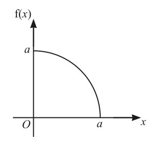
The diagram shows the graph of the probability density function, $f$ , of a random variable $X$ . The graph is a quarter circle entirely in the first quadrant with centre $(0,0)$ and radius $a$ , where $a$ is a positive constant. Elsewhere $f(x) = 0$ .

(a)

Show that $a = \frac{2}{\sqrt{\pi}}$ .

2M Similar

(b)

Show that $f(x) = \sqrt{\frac{4}{\pi} - x^2}$ .

2M Similar

DifficultyMedium-Easy

Worked solution

Approach

The graph is a quarter circle centred at the origin with radius $a$ . The equation of a circle is $x^2 + y^2 = a^2$ . Substitute the value of $a^2$ from part (a) and solve for $y = f(x)$ .

Working

The equation of the circle is:

x^2 + y^2 = a^2

From part (a), $a = \frac{2}{\sqrt{\pi}}$ , so $a^2 = \frac{4}{\pi}$ .

x^2 + y^2 = \frac{4}{\pi}

Rearranging for $y^2$ :

y^2 = \frac{4}{\pi} - x^2

Since the graph is in the first quadrant, $y \geq 0$ , so we take the positive square root:

y = \sqrt{\frac{4}{\pi} - x^2}

Thus:

f(x) = \sqrt{\frac{4}{\pi} - x^2}

Answer

Shown as required.

Final answer

Shown as required

Detailed explanation

Walkthrough

The graph represents a quarter circle in the first quadrant with centre at the origin. The standard equation for a circle centred at the origin is $x^2 + y^2 = r^2$ , where $r$ is the radius. Here, the radius is $a$ , so $x^2 + y^2 = a^2$ . We substitute $a^2 = \frac{4}{\pi}$ from part (a) into this equation. Solving for $y$ gives $y = \pm\sqrt{\frac{4}{\pi} - x^2}$ . Since the graph lies in the first quadrant where $y \geq 0$ , we take the positive root. This gives the expression for $f(x)$ .

Key Takeaways

The equation of a circle centred at the origin is $x^2 + y^2 = r^2$ .
A PDF $f(x)$ corresponds to the $y$ -values on the graph.
Domain restrictions (first quadrant) determine the sign when taking square roots.

Common Mistakes

Forgetting to square the value of $a$ when substituting into the circle equation.
Including the negative root when solving for $y$ (ignoring that $f(x) \geq 0$ in the first quadrant).

Things to Be Careful About

Ensure $a^2$ is calculated correctly: $\left(\frac{2}{\sqrt{\pi}}\right)^2 = \frac{4}{\pi}$ , not $\frac{2}{\pi}$ .

Techniques used

use equation of circlesubstitute radius constantexpress y as function of x

(c)

Show that $E(X) = \frac{8}{3\sqrt{\pi^3}}$ .

4M Similar

DifficultyMedium

Worked solution

Approach

The expected value $E(X)$ for a continuous random variable with PDF $f(x)$ is given by $\int x f(x) \, dx$ over the range of $X$ . The range is $0 \leq x \leq a = \frac{2}{\sqrt{\pi}}$ . Set up the integral and evaluate it using substitution.

Working

E(X) = \int_0^{\frac{2}{\sqrt{\pi}}} x f(x) \, dx = \int_0^{\frac{2}{\sqrt{\pi}}} x \sqrt{\frac{4}{\pi} - x^2} \, dx

Use substitution. Let $u = \frac{4}{\pi} - x^2$ . Then $\frac{du}{dx} = -2x$ , so $x \, dx = -\frac{1}{2} du$ .

Change the limits:

When $x = 0$ , $u = \frac{4}{\pi} - 0^2 = \frac{4}{\pi}$ .
When $x = \frac{2}{\sqrt{\pi}}$ , $u = \frac{4}{\pi} - \left(\frac{2}{\sqrt{\pi}}\right)^2 = \frac{4}{\pi} - \frac{4}{\pi} = 0$ .

Substitute into the integral:

E(X) = \int_{\frac{4}{\pi}}^{0} \sqrt{u} \left(-\frac{1}{2}\right) du

Swap the limits and remove the negative sign:

E(X) = \frac{1}{2} \int_0^{\frac{4}{\pi}} u^{\frac{1}{2}} \, du

Integrate:

E(X) = \frac{1}{2} \left[ \frac{u^{\frac{3}{2}}}{\frac{3}{2}} \right]_0^{\frac{4}{\pi}} = \frac{1}{2} \cdot \frac{2}{3} \left[ u^{\frac{3}{2}} \right]_0^{\frac{4}{\pi}}

E(X) = \frac{1}{3} \left[ \left(\frac{4}{\pi}\right)^{\frac{3}{2}} - 0^{\frac{3}{2}} \right]

E(X) = \frac{1}{3} \left(\frac{4}{\pi}\right)^{\frac{3}{2}} = \frac{1}{3} \cdot \frac{4^{\frac{3}{2}}}{\pi^{\frac{3}{2}}}

Since $4^{\frac{3}{2}} = (\sqrt{4})^3 = 2^3 = 8$ and $\pi^{\frac{3}{2}} = \sqrt{\pi^3}$ :

E(X) = \frac{8}{3\sqrt{\pi^3}}

Answer

Shown as required.

Final answer

Shown as required

Detailed explanation

Walkthrough

The expected value $E(X)$ is calculated using the formula $\int x f(x) \, dx$ over the support of the random variable. Here, $X$ ranges from 0 to $a = \frac{2}{\sqrt{\pi}}$ . The integral is $\int_0^{\frac{2}{\sqrt{\pi}}} x \sqrt{\frac{4}{\pi} - x^2} \, dx$ . This is best solved using substitution. Let $u = \frac{4}{\pi} - x^2$ , which gives $du = -2x \, dx$ or $x \, dx = -\frac{1}{2} du$ . Changing the limits of integration simplifies the evaluation: at $x=0$ , $u=\frac{4}{\pi}$ , and at $x=\frac{2}{\sqrt{\pi}}$ , $u=0$ . The integral becomes $\frac{1}{2} \int_0^{\frac{4}{\pi}} u^{1/2} \, du$ . Integrating gives $\frac{1}{3} u^{3/2}$ evaluated from 0 to $\frac{4}{\pi}$ . Substituting the upper limit gives $\frac{1}{3} \left(\frac{4}{\pi}\right)^{3/2} = \frac{1}{3} \cdot \frac{8}{\pi^{3/2}} = \frac{8}{3\sqrt{\pi^3}}$ .

Key Takeaways

$E(X) = \int x f(x) \, dx$ for continuous random variables.
Substitution is a powerful technique for integrals involving $x$ multiplied by a function of $x^2$ .
Always change the limits of integration when using substitution, or substitute back to $x$ before evaluating.

Common Mistakes

Forgetting to change the limits of integration when using substitution.
Incorrectly integrating $u^{1/2}$ (should be $\frac{2}{3} u^{3/2}$ , not $\frac{1}{2} u^{3/2}$ ).
Simplifying $\left(\frac{4}{\pi}\right)^{3/2}$ incorrectly; remember $4^{3/2} = 8$ .

Things to Be Careful About

The negative sign from $du = -2x \, dx$ must be handled carefully, especially when swapping limits.
Ensure the final answer is in the exact form required: $\frac{8}{3\sqrt{\pi^3}}$ .

Techniques used

set up expectation integralintegrate using substitutionevaluate definite integral

Q7MediumHypothesis TestsThe Poisson Distribution

Every July, as part of a research project, Rita collects data about sightings of a particular kind of bird. Each day in July she notes whether she sees this kind of bird or not, and she records the number $X$ of days on which she sees it. She models the distribution of $X$ by $B(31, p)$ , where $p$ is the probability of seeing this kind of bird on a randomly chosen day in July.

Data from previous years suggests that $p = 0.3$ , but in 2022 Rita suspected that the value of $p$ had been reduced. She decided to carry out a hypothesis test.

In July 2022, she saw this kind of bird on 4 days.

(a)

Use the binomial distribution to test at the 5% significance level whether Rita’s suspicion is justified.

5M Similar

DifficultyMedium

Worked solution

Approach

State the null and alternative hypotheses. Since Rita suspects the probability has decreased, use a one-tailed lower-tail test. Calculate the probability of observing 4 or fewer days under $H_0$ , compare it with the 5% significance level, and draw a conclusion in context.

Working

Let $p$ be the probability of seeing the bird on a randomly chosen day in July.

H_0: p = 0.3, \quad H_1: p < 0.3

Under $H_0$ , $X \sim B(31, 0.3)$ . The $p$ -value is

P(X \leqslant 4) = \sum_{k=0}^{4} \binom{31}{k} (0.3)^k (0.7)^{31-k}

= 0.7^{31} + 31(0.7)^{30}(0.3) + \binom{31}{2}(0.7)^{29}(0.3)^2 + \binom{31}{3}(0.7)^{28}(0.3)^3 + \binom{31}{4}(0.7)^{27}(0.3)^4

= 0.00001577 + 0.0002096 + 0.0013475 + 0.0055826 + 0.016748

= 0.0239 \quad (3\text{ sf})

Since $0.0239 < 0.05$ , reject $H_0$ at the 5% significance level.

Answer

There is sufficient evidence to support Rita's suspicion that the probability of seeing this kind of bird has decreased.

Final answer

Reject H0; sufficient evidence to support Rita's suspicion that p has decreased.

Detailed explanation

Walkthrough

Rita suspects the probability has decreased, so the alternative hypothesis must be one-tailed in the lower direction: $H_1: p < 0.3$ . The null hypothesis is that the probability is still $p = 0.3$ . Under $H_0$ , the number of days on which the bird is seen follows $B(31, 0.3)$ .

To test the suspicion, we find the probability of getting a result as extreme as, or more extreme than, the observed value of 4 days. This is $P(X \leqslant 4)$ . We add the probabilities for $X = 0, 1, 2, 3, 4$ , each of the form $\binom{31}{k}(0.3)^k(0.7)^{31-k}$ . Adding these gives $0.0239$ .

Because $0.0239 < 0.05$ , the result is significant at the 5% level. We reject $H_0$ and conclude that there is sufficient evidence that the probability has decreased.

Key Takeaways

This question tests setting up one-tailed binomial hypothesis tests, calculating a lower-tail probability, comparing it with the significance level, and writing the conclusion in context.

Common Mistakes

Using a two-tailed test when the suspicion is specifically that $p$ has decreased.
Writing the hypotheses incorrectly, e.g. $H_1: p > 0.3$ .
Forgetting to include all probabilities from $X = 0$ to $X = 4$ .
Stating a definite conclusion such as " $p$ has decreased" rather than "there is sufficient evidence that..."
Giving only the final probability $0.0239$ without showing the calculation; the mark scheme only awards B1 for an unsupported answer.

Things to Be Careful About

The conclusion must be in context and must not be definite. The mark scheme requires a valid comparison of $0.0239$ with $0.05$ , and the final conclusion should mention Rita's suspicion or the probability of seeing the bird. Also note that the $p$ -value is $P(X \leqslant 4)$ , not $P(X = 4)$ .

Techniques used

state null and alternative hypothesescalculate binomial lower-tail probabilitycompare p-value with significance levelwrite conclusion in context

(b)

In July 2023, she noted the value of $X$ and carried out another test at the 5% significance level using the same hypotheses.

Calculate the probability of a Type I error.

2M Similar

DifficultyMedium-Easy

Worked solution

Approach

For a 5% one-tailed test using the same hypotheses, find the critical region by checking that $P(X \leqslant 5)$ exceeds 0.05. Then the probability of a Type I error is the probability of rejecting $H_0$ when $H_0$ is true, which is $P(X \leqslant 4)$ .

Working

From part (a), $P(X \leqslant 4) = 0.0239$ .

P(X \leqslant 5) = 0.0239 + \binom{31}{5}(0.7)^{26}(0.3)^5 = 0.0627

Since $0.0627 > 0.05$ , the critical region for the test is $X \leqslant 4$ .

Therefore,

P(\text{Type I error}) = P(X \leqslant 4 \mid p = 0.3) = 0.0239

Answer

$0.0239$

Final answer

0.0239

Detailed explanation

Walkthrough

A Type I error occurs when we reject $H_0$ even though $H_0$ is true. To know when the test rejects $H_0$ , we need the critical region. Since the test is one-tailed at 5%, we reject for small values of $X$ . We already know $P(X \leqslant 4) = 0.0239 < 0.05$ . We also check $P(X \leqslant 5) = 0.0627 > 0.05$ , so the critical region is exactly $X \leqslant 4$ .

Therefore the probability of a Type I error is the probability, under $H_0$ , that $X$ falls in the critical region: $P(X \leqslant 4) = 0.0239$ .

Key Takeaways

A Type I error probability is the probability of rejecting $H_0$ when $H_0$ is true, which equals the probability that the test statistic falls in the critical region under $H_0$ .

Common Mistakes

Confusing Type I error with Type II error.
Using $P(X \leqslant 5)$ as the Type I error probability instead of recognising that $X \leqslant 5$ is not in the critical region because its probability exceeds 0.05.
Forgetting to show that $P(X \leqslant 5) > 0.05$ to justify the critical region.

Things to Be Careful About

The mark scheme allows follow-through from part (a) only if $P(X \leqslant 4)$ was attempted and their value is less than 0.05. The final Type I error probability must be the probability of the actual critical region, not the largest tail that exceeds the significance level.

Techniques used

identify critical regioncalculate probability of Type I error

(c)

Rita models the number of sightings, $Y$ , per year of a different, very rare, kind of bird by the distribution $B(365, 0.01)$ .

4M

(i)

Use a suitable approximating distribution to find $P(Y = 4)$ .

3M Similar

DifficultyMedium-Easy

Worked solution

Approach

Use the Poisson approximation to the binomial distribution because $n$ is large and $p$ is small. Take $\lambda = np$ , then calculate the Poisson probability.

Working

Here $n = 365$ and $p = 0.01$ , so

\lambda = np = 365 \times 0.01 = 3.65

Using $Y \sim \text{Po}(3.65)$ ,

P(Y = 4) = \frac{e^{-3.65} \times 3.65^4}{4!}

= 0.192 \quad (3\text{ sf})

Answer

$0.192$

Final answer

0.192

Detailed explanation

Walkthrough

We have a binomial distribution $B(365, 0.01)$ . Because $n$ is large and $p$ is small, the Poisson approximation is appropriate. The parameter is $\lambda = np = 365 \times 0.01 = 3.65$ .

For a Poisson distribution, $P(Y = 4) = e^{-\lambda} \lambda^4 / 4!$ . Substituting $\lambda = 3.65$ gives $e^{-3.65} \times 3.65^4 / 4! = 0.192$ to 3 significant figures.

Key Takeaways

The Poisson approximation to the binomial uses $\lambda = np$ and is valid when $n$ is large and $p$ is small. The Poisson probability formula is $P(Y = r) = e^{-\lambda} \lambda^r / r!$ .

Common Mistakes

Using the binomial formula directly instead of the Poisson approximation.
Using the wrong value of $\lambda$ , such as $\lambda = 0.01$ or $\lambda = 365$ .
Forgetting the factorial in the denominator.
Giving an unsupported answer; the mark scheme requires the expression to be seen.

Things to Be Careful About

The mark scheme states that using the binomial distribution gives $0.193$ and scores only B1. Also, $0.192$ with no working scores only B1 B1, so show the Poisson expression.

Techniques used

choose Poisson approximationcalculate lambda as npevaluate Poisson probability

(ii)

Justify your approximating distribution in this context.

1M Similar

Mathematics 9709/61 — May/June 2024

Approach

Working

Answer

Walkthrough

Key Takeaways

Common Mistakes

Things to Be Careful About

Approach

Working

Answer

Walkthrough

Key Takeaways

Common Mistakes

Things to Be Careful About

Approach

Working

Answer

Walkthrough

Key Takeaways

Common Mistakes

Things to Be Careful About

Approach

Working

Answer

Walkthrough

Key Takeaways

Common Mistakes

Things to Be Careful About

Approach

Working

Answer

Walkthrough

Key Takeaways

Common Mistakes

Things to Be Careful About

Approach

Working

Answer

Walkthrough

Key Takeaways

Common Mistakes

Things to Be Careful About

Approach

Working

Answer

Walkthrough

Key Takeaways

Common Mistakes

Things to Be Careful About

Approach

Working

Answer

Walkthrough

Key Takeaways

Common Mistakes

Things to Be Careful About

Approach

Working

Answer

Walkthrough

Key Takeaways

Common Mistakes

Things to Be Careful About

Approach

Working

Answer

Walkthrough

Key Takeaways

Common Mistakes

Things to Be Careful About

Approach

Working

Answer

Walkthrough

Key Takeaways

Common Mistakes

Things to Be Careful About

Approach

Working