Mathematics 9709/71 — May/June 2010

Cambridge A-Level · Probability & Statistics 2 · worked solutions for every part, with the mark scheme

questions

marks

minutes

Topics Continuous Random Variables · Sampling and Estimation · Hypothesis Tests · Linear Combinations of Random Variables · The Poisson Distribution

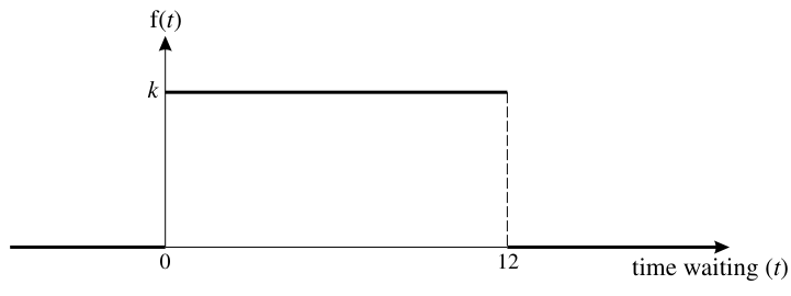
Q1Continuous Random VariablesFree sample

Fig. 1

Fred arrives at random times on a station platform. The times in minutes he has to wait for the next train are modelled by the continuous random variable for which the probability density function $f$ is shown above.

(i)

State the value of $k$ .

DifficultyEasy

Worked solution

Approach

The total area under any probability density function must equal 1. Since the graph is a rectangle, we can calculate the area as width times height.

Working

\text{Area} = 12 \times k = 1

Solving for $k$ :

k = \frac{1}{12}

Answer

k = \frac{1}{12}

Final answer

1/12

Detailed explanation

Walkthrough

A fundamental property of any probability density function (PDF) is that the total area under the curve must equal 1, representing the total probability of all possible outcomes. Here, the PDF is a rectangle with width 12 (from $t=0$ to $t=12$ ) and height $k$ . Setting the area $12k$ equal to 1 gives $k = 1/12$ .

Key Takeaways

The total area under a PDF is always 1.
For a uniform distribution (constant PDF), the height is $1/(b-a)$ where $[a, b]$ is the range.

Common Mistakes

Forgetting that the total probability must be 1.
Using the wrong width for the rectangle.

Things to Be Careful About

Ensure the units are consistent. Here $t$ is in minutes, so the area is in minutes $\times$ (1/min) = dimensionless, which is correct for probability.

Techniques used

apply the property that total area under PDF is 1calculate the constant k

(ii)

Explain briefly what this graph tells you about the arrival times of trains.

DifficultyEasy

Worked solution

Approach

The probability density function is constant ( $f(t) = k$ ) for $0 \leq t \leq 12$ . This indicates a uniform distribution, meaning the waiting time is equally likely to be any value in this range. This implies that trains arrive at regular, fixed intervals.

Working

Since the maximum waiting time is 12 minutes and the distribution is uniform (constant probability density), trains must arrive every 12 minutes. If they arrived less frequently, the waiting time could exceed 12 minutes. If they arrived more frequently, the waiting time range would be smaller.

Answer

Trains arrive every 12 minutes.

Final answer

Trains arrive every 12 minutes

Detailed explanation

Walkthrough

The graph shows a uniform distribution for the waiting time $t$ between 0 and 12 minutes. A uniform distribution means that every waiting time in this range is equally likely. In a real-world scenario like train arrivals, a uniform waiting time distribution typically arises when trains run on a fixed schedule at regular intervals. Since the waiting time ranges from 0 (arriving just as the train leaves) to 12 (arriving just after the previous train left), the interval between trains must be 12 minutes.

Key Takeaways

A uniform PDF implies equally likely outcomes within a range.
In transport contexts, a uniform waiting time suggests regular, fixed-interval scheduling.

Common Mistakes

Stating 'trains arrive randomly' (this is a uniform distribution, not necessarily random arrival times of trains, but random arrival of the passenger). The question says 'Fred arrives at random times', which leads to the uniform waiting time if trains are on a fixed schedule.

Things to Be Careful About

The mark scheme requires the phrase 'every 12 minutes'. Simply stating 'trains arrive at 12 minute intervals' is also acceptable, but the key is the regularity and the 12-minute period.

Techniques used

interpret uniform distributionrelate waiting time to train frequency

The rest of this paper

6 more questions

Q2Sampling and Estimation7M
Q3Sampling and Estimation · Hypothesis Tests7M
Q4Linear Combinations of Random Variables8M
Q5Continuous Random Variables8M
Q6The Poisson Distribution · Linear Combinations of Random Variables8M
Q7Hypothesis Tests · The Poisson Distribution10M

Loading the full paper…