Economics 9708/22 — October/November 2024
Cambridge AS Level · AS Level Data Response and Essays · worked solutions for every part, with the mark scheme
Topics Economic Growth · Balance of Payments · Protectionism · Income and Wealth Inequality · Classification of Goods and Services · Demand and Supply · +6 more
Can economic growth in Chile reduce income and wealth inequality?
Chile is the world’s biggest copper producer with 28% of global copper production and the second biggest producer of lithium with 22% of world production. Overall, mining contributes 11% of the country’s Gross Domestic Product (GDP) and more than 50% of the value of the country’s total exports. World copper and lithium prices have increased quickly since 2020. This has led to strong growth in GDP which is expected to increase by 3.5% in 2022, exceeding earlier estimates of 2.5% as world demand is expected to grow following the Covid-19 pandemic. Fig 1.1 shows the world price of copper in United States dollars (US$) per pound (lb) weight. A pound is 454 grammes.
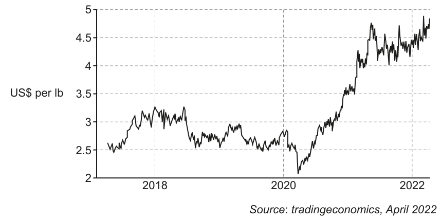
Fig 1.1: World copper price, 2017 to 2022
Source: tradingeconomics, April 2022
Economic growth in Chile has also been helped by the world’s highest rate of vaccination against Covid-19 and a rapid economic recovery from the pandemic which has led to a large increase in consumer spending.
However, the trade in goods surplus has fallen substantially in February 2022. This is mainly because of a 9.2% fall in the revenue from copper exports due to the higher prices and a fall in world demand during the Covid-19 pandemic. There has also been a 38.3% increase in the value of imported consumer goods. As a consequence, the current account deficit has widened substantially to US$7.5bn in the first quarter of 2022 from a deficit of US$1.1bn in the first quarter of 2021 despite a surplus of US$50m in the secondary income account.
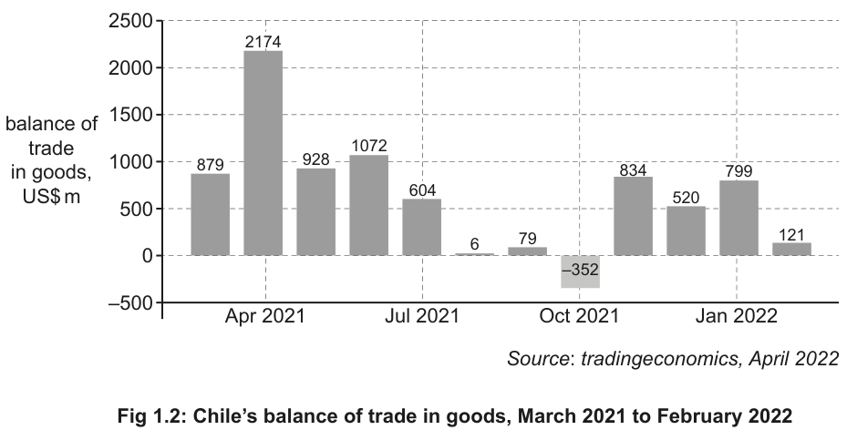
Fig 1.2: Chile’s balance of trade in goods, March 2021 to February 2022
Source: tradingeconomics, April 2022
One of the main benefits of Chile’s increased prosperity in recent years has been a decline in the number of people living at or below the minimum income level of US$5.50 per day. However, Chile remains the most unequal country in the list of largely developed countries according to the Organisation for Economic Co-operation and Development (OECD) with an income gap 65% wider than the OECD average. In addition, although the Gini coefficient has fallen from 52.1 to 44.4, this is still higher than lower-income countries such as Haiti and El Salvador.
To try and reduce this inequality in income and wealth, the Chilean government has increased its expenditure on education from 3% of GDP in 1997 to 5.4% in 2018. Further recognition of the importance of education as a merit good is shown by the government increasing its education spending by 3.4% each year since 2018. Chile has also recently made all college tuition free of charge. It is hoped that this will reduce the gap in the quality of education received by the wealthiest and poorest students and open up opportunities for everyone.
Sources: Adapted from reuters.com 2 February 2022, trade.gov/country-commercial-guides/chile-mining, 25 January 2022, bcentral.cl/inicio and statista.com, April 2022
Identify two possible reasons why the current account on the balance of payments in Chile is in deficit in the first quarter of 2022 despite the surplus on the balance of trade in goods.
Answer
-
The primary income account is in deficit. This account records net income from investments abroad and earnings of residents working overseas; a deficit here means more income is flowing out of Chile than flowing in.
-
The balance of services is in deficit. The current account includes trade in services (such as tourism and financial services), and a deficit here means Chile is importing more services than it is exporting.
A deficit on the primary income account and a deficit on the balance of services.
Background Concept
The balance of payments is a record of all economic transactions between a country and the rest of the world. The current account is a major component and consists of four sub-accounts: the balance of trade in goods, the balance of trade in services, the primary income account (investment income and compensation of employees), and the secondary income account (transfers such as foreign aid and remittances). A current account deficit means the country is spending more on foreign trade than it is earning.
Understanding the Question
The extract states that Chile's trade in goods balance is in surplus (though it has fallen), and the secondary income account is in surplus (US$50m). Yet the overall current account is in deficit (US$7.5bn). The question asks why the current account is in deficit despite the goods surplus. This requires understanding that the current account is broader than just trade in goods.
Approach
Use the accounting identity of the current account to deduce which other components must be in deficit. Since the extract explicitly mentions the secondary income surplus and the goods surplus, the deficit must come from the primary income account and/or the services balance.
Step-by-Step Reasoning
The current account balance is calculated as:
Current account = Balance of trade in goods + Balance of trade in services + Primary income + Secondary income.
Given:
- Balance of trade in goods: surplus (though reduced)
- Secondary income: surplus of US$50m
- Overall current account: deficit of US$7.5bn
For the overall balance to be negative, the sum of the goods surplus and secondary surplus must be outweighed by deficits elsewhere. Therefore, either the primary income account or the balance of services (or both) must be in deficit. The primary income account could be in deficit due to profit repatriation by foreign mining companies or high external debt servicing. The services balance could be in deficit due to high spending on imported services such as tourism, insurance, or transport.
Key Takeaways
The current account is not the same as the trade balance. A country can have a trade surplus but a current account deficit if other components (services, primary income) are sufficiently negative.
Common Mistakes
Confusing the trade in goods balance with the current account; forgetting that the current account includes services and income flows.
Things to Be Careful About
The extract mentions a 38.3% increase in imported consumer goods. This affects the trade in goods balance, not the services balance. However, the trade in goods is still in surplus, so this factor alone does not explain the current account deficit unless combined with a primary income or services deficit.
Consider the likely success of one policy that Chile could use to reduce the imports of consumer goods.
Answer
One policy is the imposition of a tariff on imported consumer goods. A tariff is a tax on imports, which raises the domestic price of these goods. This higher price reduces the quantity demanded of imports, thereby lowering expenditure on imported consumer goods.
The success of this policy depends on the price elasticity of demand (PED) for imports. If demand is price inelastic, the percentage fall in quantity demanded will be smaller than the percentage rise in price, so total expenditure on imports may not fall and could even increase. If demand is price elastic, the tariff will successfully reduce import expenditure. Therefore, the likely success is uncertain and depends on the elasticity of the specific goods being imported.
A tariff could reduce imports if demand is price elastic, but its success is uncertain if demand is inelastic.
Background Concept
Protectionism refers to government policies that restrict imports to protect domestic industries. A tariff is a specific tax levied on each unit of an imported good. It raises the domestic price of the import, leading to a movement along the demand curve for imports (a contraction in demand). The effectiveness of a tariff in reducing import expenditure depends on the price elasticity of demand for the imported goods.
Understanding the Question
The question asks for a policy to reduce imports of consumer goods and to consider its likely success. This requires identifying a policy, explaining its mechanism, and evaluating its effectiveness.
Approach
Choose a clear policy such as a tariff or quota. Explain the transmission mechanism from policy to reduced imports. Then evaluate based on the price elasticity of demand for imports, and possibly other factors such as retaliation or availability of substitutes.
Step-by-Step Reasoning
A tariff shifts the supply curve of imports vertically upwards by the amount of the tax. The new equilibrium shows a higher price and lower quantity. The change in total expenditure (price x quantity) depends on elasticity:
- If PED > 1 (elastic), the percentage fall in quantity exceeds the percentage rise in price, so expenditure falls.
- If PED < 1 (inelastic), expenditure rises.
Since many consumer goods (such as essential items or goods with few substitutes) may have inelastic demand, a tariff could fail to reduce import expenditure and might even increase it, while also raising prices for consumers. Alternative policies include quotas (physical limits) or supply-side policies to improve domestic competitiveness.
Key Takeaways
The effectiveness of demand-reduction policies depends on elasticity. Protectionism can reduce imports only if demand is responsive to price changes.
Common Mistakes
Forgetting to evaluate the policy's success; assuming all tariffs reduce imports regardless of elasticity; confusing a tariff with a quota.
Things to Be Careful About
Always link the evaluation to a specific criterion (elasticity). Mention that tariffs may invite retaliation and raise consumer prices.
Answer
The Gini coefficient is a statistical measure of income inequality within a population, ranging from 0 (perfect equality, where everyone has the same income) to 1 or 100 (perfect inequality, where one person has all the income). The fall in Chile's Gini coefficient from 52.1 to 44.4 indicates that income distribution has become more equal; the gap between the richest and poorest households has narrowed.
The fall means income is more equally distributed in Chile.
Background Concept
The Gini coefficient is the most widely used measure of inequality. It is derived from the Lorenz curve, which plots the cumulative share of income against the cumulative share of the population. The Gini coefficient equals the area between the line of perfect equality and the Lorenz curve, divided by the total area under the line of perfect equality. A higher Gini coefficient indicates greater inequality.
Understanding the Question
The question asks what is meant by the fall in the Gini coefficient from 52.1 to 44.4. This requires defining the Gini coefficient and interpreting the direction of change.
Approach
Provide a concise definition, then explain that a fall means the distribution of income has become more equal. Mention that while the fall is an improvement, the level remains high by international standards.
Step-by-Step Reasoning
Definition: The Gini coefficient measures the degree of income inequality in a country.
Interpretation: A fall from 52.1 to 44.4 means that the distribution of income across the population has become more equal. The richest households have seen their share of total income fall relative to the poorest, or the poorest have seen their share rise. However, a Gini of 44.4 is still very high compared to most developed economies, indicating that substantial inequality remains.
Key Takeaways
The Gini coefficient summarises inequality in a single number; lower values mean greater equality. Changes in the coefficient show whether inequality is rising or falling.
Common Mistakes
Confusing the Gini coefficient with measures of absolute poverty; thinking a higher number means more equality; failing to explain the direction of change.
Things to Be Careful About
The coefficient is usually expressed as a decimal (0.521) or a whole number (52.1). The extract uses 52.1, so interpret it accordingly. Always state that lower means more equal.
Assess the extent to which ‘the government increasing its education spending’ may improve the incomes of poorer households in Chile.
Answer
Increased government spending on education can improve the incomes of poorer households. Education is a merit good that yields positive externalities and is often under-consumed due to imperfect information. By increasing spending and making college tuition free, the government makes education more affordable and accessible to low-income families. This enables poorer students to acquire skills and qualifications, raising their productivity and future earning potential. Additional spending may also reduce other costs of education and raise awareness of its benefits among poorer households.
However, there are limitations. Poorer households may face high opportunity costs, as children may need to work to support the family, making free tuition alone insufficient. Information failure may persist if families do not understand the long-term benefits of education. Moreover, if spending is unsustainable, it may be cut in the future, undermining long-term gains.
In evaluation, the policy's success depends on addressing these barriers. Free tuition helps only if students can afford the opportunity cost of studying. The time lags are considerable: it takes years for current students to enter the workforce with higher skills. Therefore, while increased education spending is a valuable long-term strategy to reduce inequality, it is unlikely to rapidly improve incomes on its own and must be accompanied by targeted support for poorer households.
Increased education spending can improve incomes of poorer households in the long run by raising human capital, but its effectiveness is limited by opportunity costs, information failure, and sustainability concerns; it must be part of a broader package of measures.
Background Concept
Education is classified as a merit good because it generates positive externalities—benefits to society beyond the private benefits to the individual (such as higher productivity, lower crime, and better civic participation). Due to imperfect information, individuals may under-invest in education, especially poorer households who cannot afford the direct costs or the opportunity cost of foregone earnings. Government intervention through increased spending and free tuition aims to correct this market failure and improve equity.
Human capital theory suggests that education increases the skills and productivity of the workforce, leading to higher wages and greater social mobility. For poorer households, access to quality education is a key pathway out of poverty.
Understanding the Question
The question asks to assess the extent to which increased government education spending may improve the incomes of poorer households in Chile. This requires analysing both the potential benefits and the limitations, then reaching a judgement on the extent of the impact.
Approach
Develop two sides:
- Benefits: merit good arguments, increased access, higher productivity and wages, reduced inequality of opportunity.
- Limitations: opportunity costs, information failure, sustainability, quality of provision, time lags.
Then evaluate by weighing these factors and reaching a justified conclusion on the extent of impact.
Step-by-Step Reasoning
Benefits chain:
- Government spending increases the availability and quality of education.
- Free college tuition removes financial barriers for poorer students.
- Better education raises human capital, increasing productivity.
- Higher productivity leads to higher wages for poorer households.
- This reduces income inequality and improves living standards.
Limitations chain:
- Poorer households may still cannot afford to send children to school due to opportunity costs (lost income from child labour).
- Information failure: families may not recognise the long-term benefits of education.
- Government budget constraints: spending may be unsustainable, leading to future cuts or higher taxes.
- The quality of education matters: simply increasing spending does not guarantee better outcomes if funds are misallocated.
Evaluation:
The extent of improvement is limited in the short run due to time lags. It is more effective as a long-term structural policy. The policy is necessary but not sufficient; it must be combined with grants, childcare support, and minimum wage policies to address immediate poverty. Therefore, the extent is moderate to high in the long run but low in the short run.
Key Takeaways
Education spending addresses the supply-side root causes of inequality by building human capital, but its impact on current incomes is delayed and depends on overcoming non-cost barriers such as opportunity costs and information failure.
Common Mistakes
One-sided answers that only list benefits or only limitations; forgetting to include a conclusion; confusing education spending with immediate cash transfers; not linking the analysis specifically to poorer households.
Things to Be Careful About
Always assess the 'extent'—do not simply say 'it will improve incomes' or 'it will not'. Acknowledge both sides and reach a nuanced verdict. Mention the time lag between investment and higher income.
Assess the likely impact of the rise in the world copper price from 2020 on the future economic growth of Chile.
Answer
The rise in the world copper price from 2020 is likely to have a positive impact on Chile's future economic growth. Mining contributes more than 50% of export value and 11% of GDP, with copper being the dominant product. Assuming demand for copper is price inelastic, higher world prices will increase export revenue, which directly raises aggregate demand through the net exports component (X - M). This increase in AD will lead to higher real output and economic growth, supported by the post-pandemic recovery in world demand.
However, there are significant risks. The extract shows that revenue from copper exports fell by 9.2% in February 2022 despite higher prices, suggesting that demand for copper may be price elastic or that world demand fell during the pandemic. If demand is elastic, further price rises could reduce export revenue and GDP. Additionally, copper is a finite resource; extensive mining may lead to depletion, reducing future export capacity and growth. Higher prices may also attract new competitors, eroding Chile's market share.
In evaluation, the impact depends on the sustainability of the price rise and the elasticity of demand. The February 2022 revenue fall was likely temporary, reflecting a short-run demand shock during the pandemic. As the global economy recovers, demand and revenue should rise again, supporting growth. However, over-reliance on a single finite resource creates vulnerability to price volatility and depletion. Therefore, while the copper price rise will boost growth in the short to medium term, Chile must diversify its economy to ensure sustainable long-run growth.
The rise in copper prices will likely boost short-to-medium-term growth through higher export revenue, but long-run growth is threatened by resource depletion and price volatility unless the economy diversifies.
Background Concept
Economic growth is an increase in real GDP over time. For an open economy like Chile, growth is heavily influenced by export performance, particularly of primary commodities. The relationship between world commodity prices and national income depends on the price elasticity of demand for the export. If demand is price inelastic, higher prices raise export revenue and contribute to growth. If demand is elastic, higher prices reduce revenue.
The 'resource curse' or 'paradox of plenty' suggests that countries heavily reliant on finite natural resources may experience volatile growth, corruption, and neglect of other sectors.
Understanding the Question
The question asks to assess the likely impact of the rise in the world copper price from 2020 on the future economic growth of Chile. This requires analysing both the positive effects (higher export revenue, GDP contribution) and negative effects (revenue volatility, finite resource, competition), then evaluating the net impact on future growth.
Approach
Develop two sides:
- Positive impact: export revenue increases, AD rises, GDP grows, multiplier effects.
- Negative impact: revenue may fall if demand is elastic (as shown in Feb 2022 data), resource depletion, vulnerability to price shocks, lack of diversification.
Evaluate by weighing short-run benefits against long-run sustainability and volatility risks.
Step-by-Step Reasoning
Positive chain:
- Copper accounts for >50% of exports and 11% of GDP.
- Higher world prices increase the value of copper exports.
- If PED for copper is inelastic (as is typical for commodities with few substitutes in the short run), revenue rises.
- Higher export revenue increases AD (X rises), leading to higher real output and employment.
- The multiplier effect amplifies this growth as increased income leads to further consumption.
Negative chain:
- The extract shows export revenue fell 9.2% in Feb 2022 despite higher prices, implying either elastic demand or a demand collapse during the pandemic.
- If demand is elastic, further price rises will reduce revenue and GDP.
- Copper is finite; depletion will eventually reduce export capacity.
- High copper prices may incentivise other producers (e.g., Peru, China) to increase supply, reducing Chile's market share.
- Over-reliance on mining may cause 'Dutch disease', where the exchange rate appreciates, harming other export sectors.
Evaluation:
The February 2022 data shows that price rises do not automatically guarantee revenue growth; demand conditions matter. However, this fall was likely temporary due to pandemic-related demand shocks. In the future, as demand recovers, higher prices should support growth. The main constraint is the finite nature of copper reserves. Therefore, the impact on future growth is positive in the short to medium term but negative in the long term unless Chile diversifies its economy into other sectors and develops its non-mining export capacity.
Key Takeaways
Commodity price booms can stimulate growth but create vulnerability. Sustainable growth requires economic diversification to reduce reliance on finite resources.
Common Mistakes
One-sided answers focusing only on the benefits or only the risks; ignoring the specific data showing revenue fell despite higher prices; assuming all price rises increase revenue without considering elasticity; forgetting that copper is a finite resource.
Things to Be Careful About
Always distinguish between a rise in price and a rise in revenue—they are not the same. Use the extract's data (Feb 2022 revenue fall) to support the analysis. Consider both short-run and long-run effects.
With the help of a diagram(s), briefly explain how the cause of a movement along the demand curve differs from the cause of a shift in the demand curve and consider the impact on the demand for one good of price changes in other goods.
Answer
A movement along the demand curve is caused by a change in the price of the good itself. A fall in price from P1 to P2 leads to an expansion in quantity demanded from Q1 to Q2 along the same demand curve D1. A shift in the demand curve is caused by a change in a non-price factor, such as a rise in consumer income, which increases demand at every price, shifting the curve rightwards from D1 to D2.
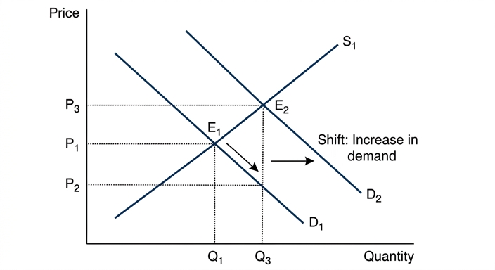
A change in the price of another good affects the demand for the first good through the relationship of substitutes or complements. If the other good is a substitute (e.g. tea for coffee), a rise in the price of the substitute increases the demand for the first good, shifting its demand curve rightwards. If the other good is a complement (e.g. printers for computers), a rise in the price of the complement reduces the demand for the first good, shifting its demand curve leftwards.
The overall impact on the demand for one good from price changes in other goods depends on the size of the cross elasticity of demand (XED) coefficient. A large positive XED indicates a strong substitute relationship, so a given price rise in the other good will cause a large increase in demand. A small negative XED indicates a weak complement relationship, so the impact will be small. Therefore, the magnitude of the effect is determined by the strength of the relationship between the goods.
A movement along the demand curve is caused by a change in the good's own price, while a shift is caused by a change in a non-price factor. The impact of price changes in other goods on demand depends on whether they are substitutes or complements, and the size of the effect is determined by the XED coefficient.
Background Concept
The demand curve shows the relationship between the price of a good and the quantity demanded, ceteris paribus. A movement along the curve occurs only when the price of the good itself changes. A shift of the entire curve occurs when any other determinant of demand changes, such as income, tastes, or the price of related goods. Related goods are classified as substitutes (goods that can replace each other, e.g. tea and coffee) or complements (goods used together, e.g. cars and petrol). The cross elasticity of demand (XED) measures the responsiveness of demand for one good to a change in the price of another: XED = % change in quantity demanded of good A / % change in price of good B. A positive XED indicates substitutes; a negative XED indicates complements. The size of the coefficient indicates the strength of the relationship.
Understanding the Question
This is an 8-mark point-based question split across three assessment objectives: AO1 (3 marks), AO2 (3 marks), and AO3 (2 marks). The question has two parts. First, it asks you to explain the difference between the cause of a movement along the demand curve and the cause of a shift in the demand curve, using a diagram. Second, it asks you to 'consider' the impact on the demand for one good of price changes in other goods. The 'consider' clause is the AO3 evaluation element, requiring a short judgement. The mark scheme explicitly warns that references to changes in income, fashion, or tastes should not be rewarded for the second part — the focus must be on price changes in other goods and the substitute/complement relationship.
Approach
For AO1, draw a single demand diagram (or two separate diagrams) that clearly shows a movement along the curve (a change in price leading to a change in quantity demanded) and a shift of the curve (a change in a non-price factor). Label the axes, the curves, and the relevant points. Explain the cause of each in words. For AO2, analyse the impact of a price change in another good on the demand for the first good, distinguishing between substitutes and complements. Use examples to illustrate. For AO3, evaluate the overall impact by introducing the concept of XED — the size of the coefficient determines the magnitude of the effect. Conclude with a short justified statement.
Step-by-Step Reasoning
-
AO1: Movement along the demand curve. Draw a demand curve D1. Show a fall in price from P1 to P2. This causes an expansion in quantity demanded from Q1 to Q2 along the same curve. The cause is a change in the good's own price. Alternatively, a rise in price would cause a contraction. The key point is that the curve itself does not move.
-
AO1: Shift of the demand curve. Draw a second demand curve D2 to the right of D1. This shows an increase in demand at every price. The cause is a change in a non-price factor, such as a rise in income, a change in tastes, or a change in the price of a related good. The curve shifts; the price of the good itself has not changed.
-
AO2: Impact of price changes in other goods — substitutes. If good B is a substitute for good A (e.g. tea and coffee), a rise in the price of good B makes good A relatively cheaper. Consumers switch from B to A, increasing the demand for A. This is shown as a rightward shift of the demand curve for A. Example: if the price of coffee rises, the demand for tea increases.
-
AO2: Impact of price changes in other goods — complements. If good B is a complement for good A (e.g. printers and computers), a rise in the price of good B makes the combined consumption of A and B more expensive. Consumers buy less of B, and therefore also less of A, reducing the demand for A. This is shown as a leftward shift of the demand curve for A. Example: if the price of printers rises, the demand for computers falls.
-
AO3: Evaluation using XED. The size of the impact depends on the cross elasticity of demand. If XED is large and positive (strong substitutes), a given price rise in the other good will cause a large increase in demand for the first good. If XED is small and negative (weak complements), the impact will be small. Therefore, the overall impact is not uniform; it depends on the specific relationship and the magnitude of the XED coefficient. A justified conclusion is that the impact is determined by the strength of the substitute or complement relationship.
Key Takeaways
- A movement along the demand curve is caused by a change in the good's own price; a shift is caused by a change in a non-price factor.
- Price changes in other goods affect demand through the substitute or complement relationship.
- The magnitude of the effect is measured by cross elasticity of demand (XED).
- For evaluation, always consider the size of the coefficient, not just the direction.
Common Mistakes
- Confusing a movement along the curve with a shift of the curve. A change in price causes a movement; a change in any other determinant causes a shift.
- Discussing changes in income or tastes for the second part of the question. The mark scheme explicitly excludes these — the focus must be on price changes in other goods.
- Only analysing one relationship (substitutes or complements) and not the other. The mark scheme caps at 2 marks for AO2 if only one is analysed.
- Omitting the diagram entirely or drawing it without labels. The question says 'with the help of a diagram', so a diagram is required for full marks.
- Forgetting the evaluation element. The 'consider' clause is the AO3 part, and up to 2 marks are reserved for it. A short judgement using XED is needed.
Things to Be Careful About
- Label the axes of the diagram correctly: price on the vertical axis, quantity on the horizontal axis.
- Clearly show the movement (arrow along the curve) and the shift (arrow from D1 to D2).
- Use specific examples for substitutes and complements to make the analysis concrete.
- For the evaluation, mention XED explicitly and explain how its size determines the magnitude of the impact.
- Keep the answer focused on the question — do not stray into other determinants of demand.
Assess whether knowledge of income elasticity of demand or price elasticity of demand for its product is more useful to a business aiming to increase the total expenditure on its product during a period of economic growth.
Introduction
Income elasticity of demand (YED) measures the responsiveness of quantity demanded to a change in income, while price elasticity of demand (PED) measures the responsiveness to a change in the good's own price. During a period of economic growth, incomes are rising, which may also put upward pressure on prices. A business aiming to increase total expenditure (revenue) must decide which elasticity is more useful for its pricing and production decisions.
The case for YED being more useful
During economic growth, rising incomes directly affect demand. YED allows a business to classify its product as a normal good (YED > 0) or an inferior good (YED < 0). For a normal good with a high YED (luxury), demand will rise significantly as incomes grow, so the business can increase output and possibly raise prices to capture higher revenue. For an inferior good, demand will fall, signalling the business to diversify or reposition its product. YED therefore provides a strategic guide to which products to produce and market during a boom. For example, a luxury car manufacturer with a YED of +2.5 can expect a 10% rise in income to increase demand by 25%, justifying expansion.
The case for PED being more useful
PED directly informs pricing strategy. If demand is price inelastic (PED < 1), a rise in price increases total revenue, as the percentage fall in quantity is smaller than the percentage rise in price. If demand is elastic (PED > 1), a price cut increases revenue. During economic growth, rising demand may allow a business to raise prices without losing many customers, but the PED value determines the exact revenue outcome. PED is also more directly actionable for short-term pricing decisions than YED, which is more relevant for long-term product planning. For example, a pharmaceutical company with a PED of -0.3 can raise prices and be confident that revenue will rise.
Evaluation
Both elasticities have limitations. They are based on historical data, which may not hold during a period of rapid economic change. YED can change as a good moves from luxury to necessity status, and PED can vary along the demand curve and over time. However, the context of economic growth gives YED a strategic edge: it tells the business whether its product is well-positioned for rising incomes. PED is more useful for tactical pricing decisions, but if the business is producing an inferior good, no amount of price manipulation will reverse the fundamental decline in demand. Therefore, YED is more useful for the initial strategic decision of what to produce, while PED is more useful for the subsequent pricing decision.
Conclusion
For a business aiming to increase total expenditure during economic growth, knowledge of YED is more useful in the first instance because it identifies whether the product will benefit from rising incomes. However, once that strategic choice is made, PED becomes essential for optimising the price to maximise revenue. The most useful approach is to use both measures together, but if forced to choose, YED provides the more fundamental guidance for a growth period.
YED is more useful for the strategic decision of what to produce during economic growth, as it identifies whether the product is a normal or inferior good. PED is more useful for tactical pricing decisions once the product is chosen. The most effective approach is to use both measures together.
Background Concept
Income elasticity of demand (YED) = % change in quantity demanded / % change in income. A positive YED indicates a normal good (demand rises with income); a negative YED indicates an inferior good (demand falls as income rises). Price elasticity of demand (PED) = % change in quantity demanded / % change in price. If PED is inelastic (absolute value < 1), total revenue rises when price rises; if elastic (absolute value > 1), total revenue rises when price falls. Total expenditure (revenue) = price x quantity. Economic growth means rising real incomes, which typically increases demand for most goods and may also lead to some inflation.
Understanding the Question
This is a 12-mark levels-marked essay part (AO1+AO2 out of 8, AO3 out of 4). The question asks you to 'assess whether knowledge of YED or PED is more useful to a business aiming to increase total expenditure during a period of economic growth'. The command word 'assess' requires a two-sided evaluation and a justified conclusion. The context is crucial: economic growth means rising incomes, which directly affects YED, but may also affect prices and therefore PED. The business's objective is to increase total expenditure (revenue), not just quantity sold. The top band for AO1/AO2 requires detailed knowledge, fully developed explanations, and a well-organised response. The top band for AO3 requires a justified conclusion with developed evaluative comments.
Approach
First, define YED and PED and explain their relevance to revenue. Then develop the case for YED being more useful: it identifies whether the product is a normal or inferior good, which is critical during a period of rising incomes. Use an example. Then develop the case for PED being more useful: it directly informs pricing strategy, which is the most direct way to increase revenue. Use an example. For evaluation, compare the two: note that both rely on historical data, that YED is more strategic while PED is more tactical, and that the context of economic growth gives YED a particular advantage. Conclude with a justified judgement that YED is more useful for the initial strategic decision, but both are needed for a complete approach.
Step-by-Step Reasoning
-
Define YED and PED. YED = % change in quantity demanded / % change in income. PED = % change in quantity demanded / % change in price. Explain the significance of the sign and size of each coefficient.
-
Explain the business objective. The business wants to increase total expenditure (revenue = price x quantity). During economic growth, incomes are rising, which may increase demand for normal goods and decrease demand for inferior goods. Prices may also be rising due to demand-pull inflation.
-
Develop the case for YED. If the product is a normal good with a high YED (luxury), rising incomes will significantly increase demand. The business can increase output and possibly raise prices, both of which increase revenue. If the product is an inferior good, the business knows it must diversify or reposition. YED provides strategic direction. Example: a luxury car manufacturer with YED = +2.5 can expect a 10% income rise to increase demand by 25%.
-
Develop the case for PED. PED directly tells the business how a price change will affect revenue. If demand is inelastic, raising price increases revenue. If elastic, lowering price increases revenue. During economic growth, the business may have more pricing power due to higher demand, but the PED value determines the exact outcome. Example: a pharmaceutical company with PED = -0.3 can raise prices and be confident revenue will rise.
-
Evaluate the two measures. Both are based on historical data, which may not be accurate during a period of rapid change. YED can change as a good moves from luxury to necessity. PED can vary along the demand curve and over time. However, the context of economic growth gives YED a strategic edge: it tells the business whether its product is well-positioned for rising incomes. PED is more useful for tactical pricing decisions, but if the business is producing an inferior good, no amount of price manipulation will reverse the fundamental decline in demand. Therefore, YED is more useful for the initial strategic decision, while PED is more useful for the subsequent pricing decision.
-
Reach a justified conclusion. The most useful approach is to use both measures together. However, if forced to choose, YED provides the more fundamental guidance for a growth period because it determines whether the product will benefit from the macroeconomic trend. The conclusion must be specific to the question and justified by the reasoning.
Key Takeaways
- YED is crucial for strategic product decisions during economic growth.
- PED is crucial for tactical pricing decisions.
- Both measures have limitations, especially reliance on historical data.
- A justified conclusion must weigh the two and state which is more useful and why.
- The context of economic growth is not just background — it is central to the analysis.
Common Mistakes
- Writing a one-sided answer that only discusses one elasticity. This forfeits all evaluation marks.
- Failing to relate the analysis to the specific context of economic growth. Generic explanations of YED and PED are not enough.
- Not reaching a conclusion, or reaching a vague conclusion like 'it depends'. The top band requires a justified judgement.
- Confusing total expenditure with profit. The question is about revenue, not profit.
- Using examples that are not relevant to the context (e.g. discussing inferior goods during a recession when the question specifies growth).
Things to Be Careful About
- Define both elasticities clearly at the start.
- Use specific examples to illustrate the points.
- Ensure the evaluation is developed and not just a list of limitations. Weigh the two measures against each other.
- The conclusion must be justified by the preceding analysis, not just a restatement of both sides.
- Organise the response logically: introduction, case for YED, case for PED, evaluation, conclusion.
With the help of a production possibility curve (PPC) diagram(s), explain the difference between constant and increasing opportunity costs and consider how choices in deciding which type of goods to produce in the short run may influence future economic growth.
Working
Diagram
Explanation of difference
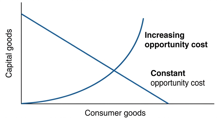
Constant opportunity cost means each additional unit of one good requires giving up the same quantity of the other good at every point on the PPC. This produces a straight-line PPC. Increasing opportunity cost means each additional unit of one good requires giving up larger and larger amounts of the other good, producing a concave (bowed-outward) PPC. The law of diminishing returns explains the increasing trade-off: as more resources are switched to producing one good, the least suitable resources are used, so the opportunity cost rises.
Influence on future economic growth
A country's choice between producing consumer goods and capital goods in the short run affects its future PPC. If it allocates more resources to consumer goods (e.g., food, entertainment), it enjoys higher current consumption but invests less in machinery, infrastructure, and technology. This limits the expansion of its PPC over time, slowing future growth. Conversely, a decision to allocate more resources to capital goods sacrifices current consumption but builds productive capacity. This shifts the PPC outward in the long run, enabling higher future consumption and sustained economic growth.
Evaluation
While capital goods are essential for long-run growth, the optimal mix depends on society's time preference and current needs. A poor country may need to prioritise immediate consumption to meet basic needs, even at the expense of future growth. A balanced approach that invests in capital goods while maintaining a minimum level of consumer goods is likely to be most effective. Thus, the trade-off is unavoidable, but an economy that neglects capital accumulation will face limited future growth.
Constant opportunity cost corresponds to a straight-line PPC; increasing opportunity cost to a concave PPC. The choice between consumer and capital goods determines the pace of future economic growth: prioritising capital goods sacrifices current consumption but shifts the PPC outward, while prioritising consumer goods boosts current output but limits long-run growth.
Background Concept
A production possibility curve (PPC) shows the maximum combinations of two goods that an economy can produce with its existing resources and technology. The shape of the PPC reflects the nature of opportunity cost. If resources are equally suited to producing either good, the trade-off is constant, giving a straight line. In reality, resources are specialised, and switching them from one use to another leads to increasing opportunity cost (diminishing returns), creating a concave curve. The slope of the PPC at any point is the marginal rate of transformation (MRT).
Economic growth is represented by an outward shift of the PPC, which requires an increase in the quantity or quality of resources or technological progress. Investment in capital goods is a key driver: current consumption forgone enables future output expansion.
Understanding the Question
Part (a) has two tasks: (i) use a PPC diagram to explain the difference between constant and increasing opportunity costs, addressing the shape of the curve and the underlying economics; (ii) ‘consider’ (which here means evaluate) how short-run choices about which goods to produce (consumer versus capital goods) affect future economic growth. The ‘consider’ clause is the AO3 element, requiring a short judgement.
Approach
Start by drawing a single diagram that shows both types of PPC: one straight line labelled ‘constant opportunity cost’ and one curved line labelled ‘increasing opportunity cost’. Clearly label axes with two different goods (e.g., ‘Consumer goods’ and ‘Capital goods’). Explain the shape difference using the law of diminishing returns.
Next, connect the choice between consumer and capital goods to growth. Use the concepts of current consumption versus investment. Show that a point on the PPC representing more capital goods corresponds to less consumer goods now but a future outward shift of the PPC.
Finally, evaluate the trade-off: it is not always optimal to maximise capital goods, as society may have urgent current needs. Offer a balanced conclusion.
Step-by-Step Reasoning
1. Diagram and shape explanation
- Draw axes: horizontal = ‘Consumer goods’, vertical = ‘Capital goods’. Draw a straight line from the vertical axis to the horizontal axis, label it ‘Constant opportunity cost PPC’. Draw a concave curve from the same vertical intercept to the same horizontal intercept? Actually, the intercepts can be the same or different; for clarity, draw both curves starting from the same point on each axis to make the shapes comparable. The straight line touches both axes; the concave curve also touches both axes but lies inside the straight line? Actually, a concave PPC that touches both axes at the same points as the straight line would be entirely inside the straight line, which implies it is less efficient. That’s not correct: both are maximum combinations. It's better to have two separate PPCs with different endpoints? But the mark scheme says “touch both axes”, so both curves must touch both axes. So draw two separate curves: one straight line, one concave, both extending from the vertical intercept to the horizontal intercept, but the concave curve will be inside the straight line? That would imply the concave curve represents fewer total possibilities? Actually, if both start at the same intercepts, the straight line lies outside the concave curve, meaning it shows a higher maximum output, which contradicts the nature of opportunity cost. The standard representation: a straight-line PPC can have different intercepts from a concave one; they are different economies. So we can draw both on the same graph but with different intercepts, or draw two separate diagrams. For clarity, describe them separately. The mark scheme seems to accept one diagram with two curves as long as they are identified.
- Explain constant opportunity cost: each extra unit of consumer goods requires giving up the same amount of capital goods (slope constant).
- Explain increasing opportunity cost: the concave shape means the opportunity cost rises as more consumer goods are produced (slope becomes steeper).
2. Link to growth
- A point on the PPC shows actual production. If the economy is at a point with more consumer goods and fewer capital goods (point C on the consumer goods axis), it is prioritising present consumption. If at a point with more capital goods and fewer consumer goods (point K near the capital goods axis), it is investing.
- Future PPC: if the economy invests in capital goods (at point K), the PPC shifts outward because the capital stock increases, enabling more of both goods in the future. If it stays at point C, the PPC shifts slowly or not at all.
- Use an example: a developing country that builds factories and infrastructure sacrifices current living standards but achieves higher long-run growth.
3. Evaluation
- The choice is not binary: societies have different time preferences. High savings rates (e.g., East Asian 'tiger' economies) led to rapid growth, while low savings can lead to stagnation. However, if basic needs are unmet, forced saving is politically and ethically difficult.
- A balanced path: allocate enough to capital goods to ensure future growth but maintain sufficient consumer goods to meet current needs. This aligns with the concept of sustainable development.
- Conclusion: the decision involves normative trade-offs, but in general, sustained growth requires a sufficient allocation to capital goods.
Key Takeaways
- PPC shape reveals the nature of opportunity cost (constant vs increasing).
- The concave PPC is the realistic case due to diminishing returns.
- Choices on the PPC affect future production possibilities: the trade-off between current consumption and investment is central to growth theory.
- Evaluation requires weighing short-run welfare against long-run capacity.
Common Mistakes
- Drawing a PPC with concave shape but failing to label axes as specific goods (e.g., ‘Consumer goods’ and ‘Capital goods’). Mark schemes penalise axes labelled only X and Y.
- Confusing constant opportunity cost with increasing: forgetting that constant gives a straight line and increasing gives a concave curve.
- Not explaining the law of diminishing returns as the reason for increasing opportunity cost.
- Describing growth as an outward shift without linking to the investment choice.
- Only describing the consumer-capital goods trade-off without evaluating it; the ‘consider’ requires a judgement.
- Missing the diagram entirely or drawing it but not explaining it in the prose (the solution must explain what the diagram shows).
Things to Be Careful About
- Ensure both curves clearly touch both axes.
- Label the curves: ‘constant opportunity cost’ and ‘increasing opportunity cost’.
- Explain diminishing returns clearly.
- Use the term ‘capital goods’ (machines, infrastructure) rather than just ‘investment’ to ground the analysis.
- The evaluation must be a short, justified conclusion – do not just list pros and cons.
- Quote the command word ‘consider’ to make it clear the AO3 part is addressed.
Assess whether a market economy is always the best economic system to effectively answer the three basic questions of resource allocation.
Introduction
The three basic questions of resource allocation are: what to produce, how to produce, and for whom to produce. In a pure market economy, these are answered by the price mechanism through the interaction of demand and supply. A planned economy uses central planning, while a mixed economy combines elements of both. This essay assesses whether the market economy is always the best system to answer these questions effectively.
Advantages of the market economy
The price mechanism performs three key functions – signalling, incentive, and rationing – that lead to efficient outcomes. Rising prices signal excess demand and incentivise firms to increase supply, while falling prices signal excess supply and encourage contraction. Consumer sovereignty ensures that what is produced reflects consumers' preferences, because profit-seeking firms produce goods that consumers are willing to buy. Regarding how to produce, competition forces firms to use the most cost-efficient methods (profit motive). For whom to produce is determined by purchasing power: goods go to those who can and will pay the market price. This decentralised process responds quickly to changes in tastes and technology without the need for a central authority. Examples of market-driven economic growth, such as in Hong Kong and Singapore, illustrate the dynamism of market allocation.
Disadvantages of the market economy
Despite its strengths, the market economy suffers from significant failures. It underprovides public goods (e.g., national defence, street lighting) because of non-excludability and non-rivalry – the free-rider problem means private firms cannot profitably supply them. It tends to overproduce demerit goods (e.g., tobacco) and underproduce merit goods (e.g., education) because consumers lack perfect information. Externalities (pollution, congestion) are not priced by the market, leading to social costs that exceed private costs. Moreover, market economies can lead to high inequality of income and wealth as purchasing power determines the distribution of goods – the needs of the poor may be ignored. Monopoly power may restrict output and raise prices, distorting the allocative efficiency. These failures suggest that a pure market system is not always best.
Comparison with a planned economy
A centrally planned economy, such as the former Soviet Union, avoids many market failures: it can ensure provision of public goods, produce merit goods in desired quantities, set prices to reflect social costs, and reduce inequality through wage controls and universal provision. However, planning suffers from severe information and incentive problems. The central planner cannot know the infinite number of consumer preferences and production possibilities, leading to shortages, surpluses, and misallocation. Without the profit motive, firms have little incentive to be efficient or innovate, resulting in low productivity and poor quality. The collapse of many planned economies demonstrates that the market system, despite its flaws, is often superior for dynamic efficiency and consumer satisfaction.
Evaluation
The pure market economy is not always the best, because it fails to allocate resources effectively in the presence of public goods, externalities, merit/demerit goods, and inequality. A planned economy can address these but at the cost of efficiency and innovation. Therefore, the optimal answer to the three basic questions is found in a mixed economy, where the government intervenes to correct market failures (through taxes, subsidies, regulation, and direct provision) while leaving most production to the market. The appropriate degree of government intervention depends on the specific conditions of each country – its level of development, institutional capacity, and social preferences.
Conclusion
A pure market economy is not always the best system to answer the three basic questions. While the price mechanism is highly effective in many areas, market failures require state intervention to ensure an efficient and equitable allocation. A mixed economy that combines market forces with targeted government intervention is generally more effective at addressing all three questions than either extreme.
A pure market economy is not always the best system for resource allocation due to market failures such as public goods, externalities, inequality, and merit/demerit goods. A mixed economy, which combines market efficiency with government correction of failures, is typically superior in answering the three basic questions.
Background Concept
Economic systems are the institutional frameworks through which societies answer the three basic questions: what to produce, how to produce, and for whom to produce. The three main types are the market economy (allocated by the price mechanism with minimal state), the planned economy (allocated by a central authority), and the mixed economy (a combination of both). Each has strengths and weaknesses, and the question requires an assessment of whether the market economy is 'always the best'.
Understanding the Question
The command word ‘Assess’ demands a balanced evaluation of the proposition. The key phrase is ‘always the best’, which requires considering situations where the market fails and where other systems perform better. The answer must compare the market economy with at least one other system (planned or mixed). A one-sided response earns zero for AO3. The top band requires a justified conclusion addressing the specific requirement of ‘always’.
Approach
Structure the essay as follows:
- Introduction: define the three basic questions and briefly set up the comparison.
- Present the strong case for the market economy: price mechanism, consumer sovereignty, profit motive, competition, and efficiency. Use examples.
- Present the counter-case: market failures – public goods, externalities, merit/demerit goods, inequality, monopoly. Explain each failure with economic reasoning.
- Compare with a planned economy: how it can address failures but suffers from information and incentive problems. Show that it is not a perfect alternative.
- Evaluate: weigh the evidence and argue that a mixed economy is generally more effective. Provide a reasoned conclusion that acknowledges context dependence.
Step-by-Step Reasoning
1. Market economy advantages
- What to produce: prices act as signals. If demand rises, price rises, signalling profit opportunity, so firms produce more. Consumer sovereignty ensures that demand determines output.
- How to produce: competition forces firms to minimise costs (profit motive). They adopt least-cost technology.
- For whom to produce: those willing and able to pay the price receive the goods. This is efficient but may be inequitable.
- Dynamic efficiency: markets encourage innovation because successful innovators earn supernormal profits.
2. Market failures
- Public goods: non-excludable and non-rival – private firms cannot charge for them, so they would be underprovided. Example: street lighting.
- Externalities: negative externalities (pollution) lead to overproduction because private costs ignore social costs; positive externalities (education) lead to underproduction.
- Merit/demerit goods: consumers may undervalue education (merit) or overvalue cigarettes (demerit) due to imperfect information.
- Inequality: market distribution may leave the poor unable to afford necessities.
- Monopoly: firms with market power can restrict output and raise prices, causing allocative inefficiency.
3. Planned economy
- Central planner can decide to produce public goods and merit goods in socially optimal quantities, and can set prices to internalise externalities (e.g., pollution taxes). Wages and prices can be set to reduce inequality.
- However, huge information problems: planner cannot know all preferences and costs, resulting in misallocation. Without competition and profit motive, firms have little incentive to be efficient or innovate. This leads to chronic shortages, low quality, and slow growth. Historical examples: Soviet Union, North Korea.
4. Evaluation
- Neither pure market nor pure planned is perfect. The market is excellent for many private goods but fails for others. The planned system solves some failures but creates worse ones.
- A mixed economy can achieve the best of both: use markets for most goods, but government intervenes to provide public goods, regulate externalities, subsidise merit goods, tax demerit goods, and redistribute income. The precise mix depends on the country's institutions and preferences.
- Conclusion: the market is not always the best because it fails in the presence of market imperfections. The qualifier ‘always’ is too strong. The mixed economy is usually superior.
Key Takeaways
- The three basic questions are a fundamental framework for comparing economic systems.
- The market economy has strong efficiency properties but suffers from market failures.
- A one-sided answer cannot earn top marks – must discuss both advantages and disadvantages, and compare to at least one other system.
- The evaluation should lead to a justified conclusion addressing ‘always’.
- Use economic terminology: price mechanism, consumer sovereignty, externalities, public goods, etc.
Common Mistakes
- Writing a one-sided essay only praising the market or only criticising it – this loses all AO3 marks.
- Failing to compare with another system; the question explicitly asks for a comparison to assess ‘always the best’.
- Presenting a vague, indecisive conclusion such as ‘it depends’ without explaining under what conditions and which system is better.
- Not using real-world examples (e.g., Hong Kong for market, Soviet Union for planned, UK or Singapore for mixed).
- Describing market failures without explaining why they represent a failure of the market to answer the basic questions effectively.
- Poor organisation – the essay should flow logically from one side to the other.
Things to Be Careful About
- Label the three basic questions clearly in the introduction.
- Ensure each point is developed with a chain of reasoning: state the concept, explain the mechanism, and link to the question.
- Do not just list points; develop them. For example, when discussing externalities, explain how the absence of a price leads to overproduction and waste.
- For AO3, go beyond simple balancing: weigh the strengths and weaknesses and offer a reasoned judgement.
- The conclusion must be specific: reject the ‘always’ claim and justify why the mixed economy is more effective.
- Keep the essay focused on the economic concepts, not political ideology.
Explain two methods of measuring unemployment and consider the extent of the possible difficulties in obtaining an accurate measurement of unemployment.
Answer
AO1 Knowledge and understanding
- The claimant count measures the number of people claiming unemployment-related benefits. (1 mark)
- The Labour Force Survey (ILO measure) is a household survey that counts as unemployed those without a job, actively seeking work, and available to start. (1 mark)
AO2 Analysis
- The claimant count understates unemployment because it excludes those not eligible for benefits or who are discouraged from claiming. It may also overstate if claimants are not genuinely seeking work. (1 mark)
- The Labour Force Survey suffers from sampling errors, may miss certain groups, and is costly to administer. (1 mark)
- Both methods have significant limitations, so no single measure provides a perfect picture. (1 mark)
AO3 Evaluation
- The extent of difficulties is considerable: the claimant count can miss a large proportion of the unemployed, while the LFS is subject to statistical inaccuracies. However, the LFS is generally regarded as more reliable because it uses an internationally agreed definition and captures a broader range of the unemployed. (1 mark)
- Conclusion: The difficulties are significant, but the LFS provides a more accurate measure than the claimant count. Policymakers should use both measures to gain a fuller understanding. (1 mark)
The difficulties are significant, but the Labour Force Survey provides a more reliable measure than the claimant count, so the extent is moderate to high depending on the method used.
Background Concept
Unemployment is a key macroeconomic indicator. Measuring it accurately is essential for policy-making. Two main methods are used: the claimant count (administrative data) and the Labour Force Survey (household survey). Each has strengths and weaknesses.
Understanding the Question
The question asks to explain two methods of measuring unemployment and then consider the extent of difficulties in obtaining an accurate measurement. It is a point-based question with marks split across AO1 (knowledge of methods), AO2 (analysis of difficulties), and AO3 (evaluation of the extent). The command word "consider" indicates a short evaluative judgement is required.
Approach
First, identify and briefly explain the two methods (claimant count and Labour Force Survey). Then analyse the difficulties associated with each method. Finally, evaluate the overall extent of the difficulties and reach a conclusion about which method is more reliable.
Step-by-Step Reasoning
-
Claimant count: This is a count of individuals receiving unemployment benefits. It is easy to collect but excludes those not eligible (e.g., young people, long-term unemployed who have exhausted benefits) and those not claiming (discouraged workers). It may also include people who are not genuinely seeking work. Thus, it can both understate and overstate true unemployment.
-
Labour Force Survey (LFS): This is a quarterly survey of households. It uses the ILO definition: unemployed if without work, actively seeking work, and available to start. It captures a broader range of the unemployed, including those not eligible for benefits. However, it is based on a sample, so it has sampling error. It may miss certain groups (e.g., homeless) and is costly.
-
Analysis of difficulties: Both methods have flaws. The claimant count is cheap but inaccurate; the LFS is more accurate but expensive and subject to statistical error. The extent of the difficulties is significant because the claimant count can miss up to a third of the unemployed, while the LFS may have a margin of error of a few percentage points.
-
Evaluation: The LFS is generally considered more reliable because it uses a consistent definition and is less prone to administrative changes. However, it is not perfect. The extent of difficulties is moderate to high, but policymakers can use both measures to cross-check. The conclusion is that the LFS is the better measure, but both are needed for a complete picture.
Key Takeaways
- Two main measures: claimant count (administrative) and Labour Force Survey (survey-based).
- Each has specific difficulties: under/overcounting, sampling errors.
- The LFS is more accurate but not perfect.
- Evaluation requires a judgement on the extent of difficulties and a conclusion.
Common Mistakes
- Confusing types of unemployment (structural, cyclical) with methods of measurement. The question specifically asks for methods, not types.
- Only discussing one method's difficulties – the mark scheme caps at 2 marks if only one method is analysed.
- Failing to provide a conclusion – the evaluation marks require a final judgement.
- Quoting figures without interpretation – not relevant here.
Things to Be Careful About
- Ensure both methods are clearly identified and explained.
- Analyse difficulties for both methods.
- The evaluation must address the "extent" of difficulties, not just list them.
- The conclusion should be justified, not just a summary.
Assess whether supply-side policy is likely to be equally successful in reducing both structural and cyclical unemployment.
Introduction
Supply-side policy aims to increase the productive capacity of the economy by shifting the long-run aggregate supply (LRAS) curve to the right. Structural unemployment arises from a mismatch between workers' skills and job vacancies, while cyclical unemployment results from a deficiency of aggregate demand (AD). This essay assesses whether supply-side policy is equally successful in reducing both types.
Supply-side policy and structural unemployment
Supply-side policies such as education and training, infrastructure investment, and labour market deregulation directly address the causes of structural unemployment. For example, training programmes equip workers with skills needed in growing industries, reducing the mismatch. Improved infrastructure connects workers to jobs. These policies shift LRAS to the right, increasing the economy's potential output and reducing the natural rate of unemployment.
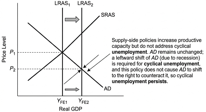
As shown in the diagram, the rightward shift of LRAS from LRAS1 to LRAS2 leads to a higher real GDP and a lower price level, indicating an increase in the economy's capacity to employ workers. Thus, supply-side policy is highly effective in reducing structural unemployment.
Supply-side policy and cyclical unemployment
Cyclical unemployment is caused by a fall in AD, leading to a recessionary gap. Supply-side policy primarily affects LRAS, not AD. Therefore, it does not directly address the demand deficiency. For instance, during a recession, even if workers are trained, there may be no jobs available because firms face low demand. Some supply-side policies, such as government spending on infrastructure, can boost AD in the short run, but this is not their primary aim. Demand-side policies (fiscal or monetary expansion) are more directly effective in reducing cyclical unemployment.
Evaluation
- Time lags: Supply-side policies take years to have an effect, whereas cyclical unemployment often requires immediate action. This limits their success for cyclical unemployment.
- Cost: Supply-side policies are expensive and may not be justified if the main problem is demand-deficient.
- Complementarity: Supply-side policy can complement demand-side policy: after demand is restored, supply-side measures can help prevent structural unemployment from rising. However, on its own, it is not equally successful.
- Context: In an economy with both structural and cyclical unemployment, supply-side policy alone will not solve the cyclical component.
Conclusion
Supply-side policy is more effective in reducing structural unemployment by directly addressing skill mismatches and increasing productive capacity. It is not equally successful for cyclical unemployment because it does not tackle deficient AD. Therefore, the statement that supply-side policy is likely to be equally successful in reducing both types of unemployment is not supported. A combination of supply-side and demand-side policies is necessary.
Supply-side policy is more effective in reducing structural unemployment by shifting LRAS right, but it is not equally successful for cyclical unemployment because it does not directly address deficient AD; therefore, the statement is not supported.
Background Concept
Supply-side policy refers to measures designed to increase the economy's productive capacity by shifting the LRAS curve to the right. Structural unemployment occurs when there is a mismatch between the skills of workers and the requirements of available jobs, often due to technological change or industrial decline. Cyclical unemployment arises from a lack of aggregate demand during economic downturns. The effectiveness of supply-side policy depends on the type of unemployment.
Understanding the Question
The question asks to assess whether supply-side policy is likely to be equally successful in reducing both structural and cyclical unemployment. This is a levels-marked essay (12 marks) requiring developed analysis and evaluation. The command word "assess" demands a two-sided argument and a justified conclusion. The top band requires detailed knowledge, fully developed explanations, and a justified conclusion addressing the specific question.
Approach
First, define key terms. Then analyse how supply-side policy can reduce structural unemployment, using an AD/AS diagram to illustrate. Next, analyse why supply-side policy is less effective for cyclical unemployment, explaining the role of AD. Then evaluate the relative effectiveness by considering time lags, cost, and complementarity with demand-side policies. Finally, reach a conclusion that answers the question directly.
Step-by-Step Reasoning
-
Structural unemployment: Supply-side policies like training and infrastructure improve labour mobility and productivity. This shifts LRAS right, increasing potential output and reducing the natural rate of unemployment. The diagram shows LRAS shifting right, with AD constant, leading to higher output and lower price level. This directly reduces structural unemployment.
-
Cyclical unemployment: This is caused by a fall in AD. Supply-side policy does not shift AD; it shifts LRAS. Therefore, even if the economy's capacity increases, if AD is insufficient, output will remain below potential and cyclical unemployment persists. For example, during a recession, training programmes do not create jobs if firms are not hiring. Some supply-side policies (e.g., government infrastructure spending) can boost AD, but this is a secondary effect and not the main purpose.
-
Evaluation:
- Time lags: Supply-side policies take years to implement and yield results, while cyclical unemployment needs immediate demand stimulus.
- Cost: Supply-side policies are expensive; using them solely for cyclical unemployment is inefficient.
- Complementarity: The best approach is to use demand-side policies to close the recessionary gap and then supply-side policies to prevent structural unemployment from rising. On its own, supply-side policy is not equally successful.
- Context: In an economy with high structural unemployment (e.g., due to deindustrialisation), supply-side policy is crucial. In a recession, it is insufficient.
-
Conclusion: Supply-side policy is more successful for structural unemployment. It is not equally successful for cyclical unemployment. Therefore, the statement is not supported.
Key Takeaways
- Supply-side policy shifts LRAS, affecting the natural rate of unemployment.
- Cyclical unemployment requires demand-side policies.
- Evaluation should consider time lags, cost, and complementarity.
- A justified conclusion must directly answer the question.
Common Mistakes
- One-sided answer: only discussing structural unemployment or only cyclical. The question requires both.
- Confusing supply-side policy with demand-side policy.
- Failing to use AD/AS analysis or not explaining the diagram.
- Providing a conclusion that is vague or does not address the "equally successful" aspect.
- Listing policies without developing the chain of reasoning.
Things to Be Careful About
- Clearly distinguish between structural and cyclical unemployment.
- Use the AD/AS diagram to show the effect on LRAS and explain it fully.
- Ensure evaluation is developed and supported, not just a list of points.
- The conclusion must be justified and specific to the question.
- Avoid generalisations; use economic terminology precisely.
With the help of examples, explain the difference between the marginal rate of taxation and the average rate of taxation and consider whether a government should decide to increase the rate of indirect tax to raise additional revenue.
Answer
Marginal rate of taxation (MRT) is the proportion of an additional unit of income that is paid in tax. For example, if a person earns an extra £100 and pays £40 in tax on that extra income, the MRT is 40%. Average rate of taxation (ART) is the total tax paid as a proportion of total income. For example, if a person earns £10,000 and pays £3,000 in tax, the ART is 30%.
The difference is that MRT focuses on the tax on extra income, while ART is the overall tax burden. In a progressive tax system, MRT > ART; in a regressive system, MRT < ART.
Consideration of increasing indirect tax to raise additional revenue:
Increasing indirect taxes (e.g., VAT) can raise revenue quickly and may be easier to administer than direct taxes. They are also harder to avoid. However, indirect taxes are often regressive, meaning they take a larger proportion of income from lower-income households, leading to a higher MRT for the poor. Their effectiveness depends on the price elasticity of demand (PED): if demand is inelastic, revenue will rise significantly; if elastic, the tax may reduce consumption and revenue may not increase as much. Additionally, indirect taxes can cause cost-push inflation.
Evaluation: While indirect taxes can be an effective way to raise revenue, their regressive nature and potential inflationary effects must be weighed against the benefits. A government should consider using a mix of taxes and may prefer progressive direct taxes to avoid worsening inequality. Therefore, increasing indirect tax is not always the best option; it depends on the government's distributional objectives and the elasticity of the goods taxed.
Conclusion: A government should only increase indirect tax if the goods have inelastic demand and if the regressive impact can be mitigated, e.g., by exempting necessities.
Indirect tax increases can be effective for raising revenue when demand is inelastic, but their regressive nature and potential for cost-push inflation mean they should not be the sole method; a balanced approach with progressive taxes is preferable.
Background Concept
Marginal rate of taxation (MRT) is the tax rate applied to the last unit of income earned. It determines the incentive to earn additional income. Average rate of taxation (ART) is the total tax paid divided by total income, reflecting the overall tax burden. In a progressive tax system, MRT > ART; in a regressive system, MRT < ART. Indirect taxes are taxes on goods and services, such as VAT, which are regressive because they take a larger proportion of income from lower-income households. The effectiveness of an indirect tax increase in raising revenue depends on the price elasticity of demand (PED): if demand is inelastic, the tax increase leads to a proportionally smaller decrease in quantity demanded, so total revenue rises; if elastic, revenue may fall.
Understanding the Question
The question has two parts: first, explain the difference between MRT and ART with examples (AO1). Second, consider whether a government should increase indirect tax to raise additional revenue (AO2 and AO3). The command word "consider" implies evaluation: you must discuss both advantages and disadvantages and reach a justified conclusion. The mark scheme allocates up to 3 marks for knowledge, 3 for analysis, and 2 for evaluation.
Approach
Start by defining MRT and ART with clear numerical examples. Then analyse the pros and cons of increasing indirect tax: advantages (quick revenue, hard to avoid) and disadvantages (regressive, depends on PED, inflationary). Finally, evaluate by weighing these factors and conclude with a judgement on when such a policy is appropriate.
Step-by-Step Reasoning
- Definitions and examples: MRT = tax on extra income / extra income. Example: extra £100, tax £40 → MRT 40%. ART = total tax / total income. Example: income £10,000, tax £3,000 → ART 30%. Explain that MRT is marginal, ART is average.
- Analysis of indirect tax increase:
- Advantages: Quick to implement, lower administrative costs, harder to evade than direct taxes (e.g., income tax), can target specific goods (e.g., tobacco).
- Disadvantages: Regressive – lower-income households spend a higher proportion of income on taxed goods, so the tax burden is heavier on them. Effectiveness depends on PED: if demand is elastic, the tax may reduce consumption significantly, possibly reducing revenue. Also, indirect taxes can increase costs of production and lead to cost-push inflation.
- Evaluation: Weigh the trade-off. If the government aims to raise revenue without worsening inequality, progressive direct taxes may be better. If the goal is to discourage consumption of demerit goods, indirect taxes are suitable. The conclusion should state that indirect tax increases are not always the best option; they are most effective when demand is inelastic and when the regressive impact can be offset (e.g., by exempting necessities or providing transfers).
Key Takeaways
- Understand the difference between marginal and average tax rates.
- Recognise the regressive nature of indirect taxes.
- Apply PED to evaluate tax policy.
- Form a balanced judgement based on economic criteria.
Common Mistakes
- Providing only one side of the argument for the indirect tax part (loses evaluation marks).
- Not using numerical examples for MRT and ART.
- Ignoring the role of PED in determining revenue impact.
- Failing to reach a clear conclusion.
Things to Be Careful About
- Ensure definitions are precise and examples are correct.
- Include both advantages and disadvantages in the analysis.
- Use the extract's context if provided (none here).
- The conclusion should be specific to the question, not generic.
Assess whether the achievement of a balanced budget should always be a main government macroeconomic objective.
Introduction
A balanced budget occurs when government revenue equals expenditure. The question asks whether achieving a balanced budget should always be a main macroeconomic objective. While a balanced budget can promote stability, it may conflict with other objectives such as economic growth and low unemployment.
Arguments for a balanced budget as a main objective
A balanced budget signals fiscal discipline, which can boost confidence among investors and consumers, leading to lower interest rates and higher investment. It avoids the accumulation of national debt, which can burden future generations. In the long run, a balanced budget is sustainable and prevents inflationary pressures from excessive government spending.
Arguments against always prioritising a balanced budget
During a recession, tax revenues fall and automatic stabilisers increase spending, leading to a deficit. Attempting to balance the budget in a recession would require contractionary fiscal policy (cutting spending or raising taxes), which would worsen the downturn and increase unemployment. Conversely, during a boom, a surplus may be desirable to cool demand and control inflation. A rigid commitment to a balanced budget would prevent this counter-cyclical policy. Additionally, a balanced budget may involve opportunity costs if it prevents necessary public investment in infrastructure or education.
Evaluation
The desirability of a balanced budget depends on the economic cycle. In a recession, a deficit is appropriate to stimulate demand; in a boom, a surplus helps control inflation. Over the cycle, a balanced budget may be a sensible long-term goal, but it should not be an inflexible target. Other objectives such as low unemployment and price stability may take priority in the short run.
Conclusion
A balanced budget should not always be a main macroeconomic objective. Its importance varies with economic conditions. Governments should aim for a balanced budget over the economic cycle but allow deficits during recessions and surpluses during booms to achieve other macroeconomic goals.
A balanced budget should not always be a main macroeconomic objective; its priority depends on the economic cycle. During recessions, deficit spending is necessary to boost demand, while during booms, surpluses may be needed to control inflation. Therefore, a balanced budget is a useful long-term goal but should be flexible in the short run.
Background Concept
A balanced budget is when government revenue equals expenditure. A budget deficit (spending > revenue) increases national debt, while a surplus (revenue > spending) reduces it. Fiscal policy can be expansionary (deficit) or contractionary (surplus). Governments have multiple macroeconomic objectives: price stability, low unemployment, economic growth, and a sustainable balance of payments. A balanced budget is not an explicit objective in many frameworks but is often seen as desirable for long-term sustainability.
Understanding the Question
The question asks to "assess whether the achievement of a balanced budget should always be a main government macroeconomic objective." The word "always" is an absolute, so the answer must challenge it. The command word "assess" requires analysis of both sides and a justified conclusion. The mark scheme is levels-based: AO1+AO2 out of 8, AO3 out of 4. Top band requires detailed knowledge, developed analysis, and a justified conclusion.
Approach
First, present the case for a balanced budget as a main objective: stability, confidence, debt avoidance. Then present the case against: need for counter-cyclical policy, opportunity costs. Evaluate by considering the economic cycle and trade-offs. Conclude that a balanced budget should not always be a main objective; it depends on conditions.
Step-by-Step Reasoning
- Arguments for: A balanced budget signals fiscal responsibility, which can lower borrowing costs and encourage investment. It prevents debt accumulation, which could crowd out private investment or require future tax increases. In the long run, it ensures sustainability.
- Arguments against: In a recession, automatic stabilisers create a deficit; trying to balance the budget would require austerity, worsening the recession (paradox of thrift). A deficit can stimulate demand through the multiplier effect. In a boom, a surplus can cool demand and prevent overheating. A rigid balanced budget rule would prevent this stabilisation. Also, a balanced budget may force cuts in productive public investment, harming long-term growth.
- Evaluation: The appropriate fiscal stance depends on the economic cycle. Over the cycle, a balanced budget may be desirable, but in the short run, deficits and surpluses are necessary tools. Other objectives like low unemployment and price stability may be more urgent. Therefore, a balanced budget should not always be a main objective; it should be one of several objectives, with priority determined by current conditions.
- Conclusion: A balanced budget is a useful long-term goal but should not be inflexible. Governments should aim for a balanced budget over the cycle, allowing deficits in recessions and surpluses in booms.
Key Takeaways
- Understand the role of fiscal policy in stabilisation.
- Recognise the trade-off between balanced budget and other objectives.
- Apply counter-cyclical fiscal policy reasoning.
- Form a nuanced conclusion that avoids absolutes.
Common Mistakes
- One-sided answer (only arguing for or against) – loses all evaluation marks.
- Not addressing the "always" in the question – failing to challenge the absolute.
- Providing a vague conclusion without justification.
- Ignoring the distinction between short run and long run.
Things to Be Careful About
- The question says "a main objective", not "the main objective". So you can argue it is one of several, but not always the priority.
- Use economic terminology: automatic stabilisers, multiplier, crowding out, counter-cyclical.
- Ensure the conclusion is specific and justified, not just a summary.
- No diagram is required, but if you use one (e.g., AD/AS showing deficit impact), it must be fully explained. Not necessary here.