Economics 9708/44 — October/November 2025
Cambridge A-Level · A Level Data Response and Essays · worked solutions for every part, with the mark scheme
Topics Market Structures · Performance of Firms in Different Market Structures · Effectiveness of Macroeconomic Policies · Efficiency and Market Failure · Externalities, Social Costs and Benefits · Utility Theory · +3 more
Market Economies
From Adam Smith onwards, most economists have regarded competitive markets as the main mechanism of economic activity. They argue that the interaction between producers and consumers can lead to both allocative efficiency and productive efficiency.
It can, however, be questioned whether the market automatically produces the best solution. Sometimes there are significant reasons for governments to intervene in a market in order to produce a better outcome than market forces alone. These situations are market failures.
When producing goods and services firms consider the private costs they pay and private benefits they receive. For example, a steel producer accounts for the cost of iron ore, fuel, labour and administration. It offsets these costs against the revenue from selling the steel. However, those people who live near the steelworks suffer the consequences of the noise, dirt and polluted air generated as part of the production process. Similarly, in many areas the extraction of iron ore can lead to environmental destruction such as the degradation of ground water for domestic consumption and a reduction in the variety of wildlife and flowers.
Competitive markets as envisaged by economists, however, may not exist. Firms may integrate to gain the benefits of economies of scale, to realise their ambition to rule the market or to increase their market share. Such integration might lead to the development of a monopoly market structure. Many believe that a monopoly always operates against the interests of the consumer because of its lack of efficiency. As a result, governments often restrict the operation of monopolies.
Answer
Allocative efficiency occurs when firms produce the goods and services that consumers want, where marginal cost equals marginal revenue (or price), i.e., MC = AR = P.
Productive efficiency occurs when goods and services are produced using the least amount of resources, which is achieved when production is on the lowest point of the average cost curve (minimum average cost), or equivalently when an economy is producing on its production possibility curve (PPC).
Background Concept
Efficiency in economics refers to the optimal production and allocation of resources. Allocative efficiency and productive efficiency are two distinct but related concepts. Allocative efficiency is concerned with producing the right mix of goods and services that match consumer preferences. It is achieved when resources are allocated in a way that maximises societal welfare, which occurs where the marginal cost of production equals the marginal benefit to consumers (price). Productive efficiency is concerned with producing goods at the lowest possible cost. It occurs when an economy or firm is operating at the minimum point of its average cost curve, meaning no resources are wasted in production. Both concepts are central to welfare economics and the analysis of market failure.
Understanding the Question
The question asks for an explanation of two specific economic efficiency concepts: allocative efficiency and productive efficiency. It is a 4-mark definition/explanation question. The command word is 'Explain', which requires more than just a definition; it requires stating the conditions under which each efficiency is achieved. The question does not ask for a diagram or evaluation, only the meaning of the two terms.
Approach
Define each term separately. For allocative efficiency, state that it is producing what consumers want and give the condition MC = AR = P (or MC = P). For productive efficiency, state that it is producing with the least use of resources and give the condition of minimum average cost (lowest point of AC curve) or production on the production possibility curve (PPC). Keep it concise and clear, covering four distinct points to match the 4-mark tariff.
Step-by-Step Reasoning
- Allocative efficiency: Start by stating that it means producing the goods and services that consumers desire. Then give the technical condition: marginal cost equals marginal revenue (or average revenue), which equals price. This ensures that the value consumers place on the last unit equals the cost of producing it.
- Productive efficiency: State that this means producing goods and services using the least amount of resources, or at the lowest possible cost. The condition is production at the minimum point of the average cost curve (minimum AC). Alternatively, it can be described as producing on the production possibility curve (PPC), indicating that all resources are fully and efficiently employed with no waste.
- Ensure both are clearly separated and each has a definition and a condition.
Key Takeaways
- Allocative efficiency = right mix of goods (MC = P).
- Productive efficiency = lowest cost production (minimum AC / on PPC).
- These are distinct concepts: one is about what to produce and for whom, the other is about how to produce.
Common Mistakes
- Confusing the two terms.
- Stating allocative efficiency as 'supply equals demand' without mentioning MC = P.
- Stating productive efficiency as 'producing at maximum output' rather than minimum cost.
- Forgetting the condition (MC=P or AC=min) which is often required for the mark.
Things to Be Careful About
- Use precise terminology: 'marginal cost equals price' or 'MC = AR = P'.
- For productive efficiency, mention 'lowest average cost' or 'minimum point of the AC curve'.
- Keep the answer balanced: roughly equal detail for both terms to reflect the equal weighting implied by the 4-mark tariff.
Answer
A negative production externality is a cost that is borne by someone other than the producer of the good, i.e., a third party.
Background Concept
Externalities are costs or benefits of economic activity that affect third parties who are not directly involved in the production or consumption of a good. They are also known as external costs or external benefits. A negative externality occurs when the external effect is harmful, imposing a cost on others. Externalities can arise from production (e.g., pollution from a factory) or consumption (e.g., passive smoking). Because the market price reflects only private costs and benefits, externalities cause a divergence between private and social costs/benefits, leading to market failure.
Understanding the Question
The question asks for an explanation of a 'negative production externality'. It is a 2-mark definition question. The key elements are: (1) it is a cost, and (2) it is borne by a third party (not the producer or consumer). The context is steel production, but the definition must be general.
Approach
Provide a concise definition covering both elements: the nature of the cost and who bears it. A negative production externality is a cost imposed on third parties outside the production process.
Step-by-Step Reasoning
- Identify that it is a cost (not a benefit).
- Identify that the cost is borne by someone other than the producer — a third party.
- Combine these into a clear sentence.
Key Takeaways
- Negative = cost (not benefit).
- Production = arises from the production process.
- Externality = affects third parties.
- The producer does not pay this cost, so it is not reflected in the market price.
Common Mistakes
- Confusing with a positive externality (benefit).
- Confusing with a private cost (borne by the producer).
- Forgetting to mention the third party.
Things to Be Careful About
- Ensure the definition explicitly mentions 'third party' or 'someone other than the producer' — this is usually the second mark.
- Keep it brief; 2 marks do not require examples or diagrams.
Identify from the extract a negative production externality resulting from steel production.
Answer
Noise, dirt or polluted air generated by the steelworks. (Alternatively: environmental destruction such as degradation of ground water, or reduction in the variety of wildlife and flowers.)
Noise, dirt or polluted air
Background Concept
Negative production externalities are widespread in industrial economies. Common examples include air and water pollution, noise pollution, and environmental degradation. When identifying an externality from a text, one must distinguish between private costs (paid by the firm, e.g., raw materials, wages) and external costs (borne by others).
Understanding the Question
The question asks to identify a negative production externality from the extract. The extract describes steel production and its consequences. The student must locate a cost imposed on third parties, not a private cost of the firm. The mark is for a specific example from the text.
Approach
Scan the extract for phrases describing harm to people or the environment that is not part of the firm's private costs. The extract mentions: 'noise, dirt and polluted air', 'environmental destruction such as the degradation of ground water for domestic consumption and a reduction in the variety of wildlife and flowers.' Any one of these is correct.
Step-by-Step Reasoning
- Read the extract carefully.
- Identify the sentence: 'those people who live near the steelworks suffer the consequences of the noise, dirt and polluted air generated as part of the production process.'
- Identify that these are costs borne by third parties (local residents), not the steel producer.
- Select one example: noise, dirt, polluted air, environmental destruction, degradation of ground water, reduction in wildlife/flowers.
- State it clearly.
Key Takeaways
- Private costs: iron ore, fuel, labour, administration (paid by the firm).
- External costs: noise, dirt, polluted air, environmental damage (paid by third parties).
- Always link the example to the specific industry in the extract.
Common Mistakes
- Giving a private cost (e.g., 'cost of iron ore' or 'labour costs') — these are not externalities.
- Being too vague ('pollution') without linking to the extract, though 'polluted air' is explicitly in the text.
- Giving more than one example when only one is needed (though it does not lose marks, it is unnecessary).
Things to Be Careful About
- The question asks for an example from the extract. Do not invent examples not mentioned.
- Ensure the example is a production externality (from making steel), not a consumption externality.
Explain, with the aid of a diagram, the consequences for output and price if the steel market is required to take into consideration negative production externalities.
Answer
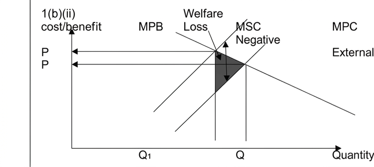
The diagram shows the market for steel with marginal private benefit (MPB) and marginal private cost (MPC). In an unregulated market, equilibrium is where MPC = MPB, at price P and quantity Q. However, steel production imposes external costs on third parties, so marginal social cost (MSC) is above MPC by the amount of the external cost.
If the steel market is required to take into account these negative production externalities, the supply curve effectively shifts leftward from MPC to MSC. The new socially optimal equilibrium is where MSC = MPB, at price P1 and quantity Q1.
Consequently, the output falls from Q to Q1 and the price rises from P to P1. The shaded triangular area between Q1 and Q, bounded by MSC and MPC (or MPB), represents the deadweight welfare loss that existed under the unregulated market.
Output falls from Q to Q1 and price rises from P to P1.
Background Concept
When a negative production externality exists, the market fails because the firm only considers its private costs (MPC) and ignores the external costs imposed on society. The social cost (MSC) is the sum of private cost and external cost. The market equilibrium (where MPC = MPB) results in overproduction and underpricing relative to the social optimum (where MSC = MPB). Government intervention, such as a tax equal to the external cost, can internalise the externality, shifting the supply curve up to reflect the true social cost. This reduces output to the socially optimal level and raises the price, but also eliminates the deadweight welfare loss (the triangle of net social harm caused by the overproduction).
Understanding the Question
The question asks for the consequences for output and price if the steel market is required to internalise negative production externalities. It is worth 5 marks and explicitly requires a diagram. The command word is 'Explain', which means a developed chain of reasoning is needed. The mark scheme awards marks for: diagram labels and axes (2 marks), indication of negative externality (1 mark), comment on quantity falling (1 mark), comment on price rising (1 mark), and explanation of welfare loss (1 mark).
Approach
Draw (or describe) a standard negative production externality diagram with MPB, MPC, and MSC. Explain the unregulated equilibrium (P, Q) and the new equilibrium after internalisation (P1, Q1). State that output falls and price rises. Explain the welfare loss triangle that existed before and is removed after.
Step-by-Step Reasoning
- Diagram: Draw cost/benefit on the vertical axis and quantity on the horizontal axis. Draw a downward-sloping MPB curve. Draw two upward-sloping curves: MPC (to the right) and MSC (to the left, indicating higher social cost). Label the vertical distance between them as the external cost. Mark the market equilibrium at the intersection of MPC and MPB (price P, quantity Q). Mark the social optimum at the intersection of MSC and MPB (price P1, quantity Q1). Shade the deadweight loss triangle between Q1 and Q.
- Explanation of unregulated market: Without intervention, firms produce where MPC = MPB. Because they ignore external costs, they overproduce at quantity Q.
- Effect of internalisation: Requiring the market to account for externalities (e.g., via a Pigouvian tax) shifts the effective supply curve from MPC to MSC.
- New equilibrium: The new equilibrium is where MSC = MPB. This occurs at a higher price (P1) and lower quantity (Q1).
- Consequences: Output falls from Q to Q1. Price rises from P to P1.
- Welfare loss: The shaded triangle between Q1 and Q represents the deadweight welfare loss that existed because the external cost was not borne by producers. Internalisation eliminates this loss.
Key Takeaways
- Negative production externalities cause overproduction and underpricing.
- Internalising the externality (e.g., tax) shifts supply left/up.
- Output falls, price rises, moving towards the social optimum.
- The welfare loss is the area between MSC and MPC over the overproduced units.
Common Mistakes
- Drawing the diagram with MSC below MPC (wrong direction).
- Forgetting to label axes or curves.
- Saying output rises or price falls (wrong direction).
- Describing the welfare loss as a rectangle instead of a triangle.
- Forgetting to explain the welfare loss.
Things to Be Careful About
- Ensure the diagram clearly shows MSC above MPC.
- Explicitly state the direction of change: quantity decreases, price increases.
- The welfare loss must be explained as the net social cost of the overproduction, not just 'a loss'.
Answer
Arguments that a monopoly may operate in the interests of consumers:
A monopoly can achieve economies of scale because it produces at a larger output than competitive firms. This lower average cost can be passed on to consumers in the form of lower prices. Additionally, monopolies may invest heavily in research and development (R&D) because they have supernormal profits to fund such investment and a longer time horizon due to protected market share. This can lead to better products for consumers. In the case of a natural monopoly, such as railways or utilities, a single firm is the most efficient structure because duplication of infrastructure would be wasteful.
Arguments that a monopoly operates against consumer interests:
A monopoly lacks allocative efficiency because it sets price above marginal cost (P > MC) to maximise profit, meaning consumers pay more than the cost of production and output is restricted below the socially optimal level. It also lacks productive efficiency because, without competitive pressure, it may not produce at the minimum point of its average cost curve (X-inefficiency). Furthermore, a monopoly may suffer from a lack of dynamic efficiency, as the absence of competitors reduces the incentive to innovate or improve products over time.
Conclusion:
A monopoly does not always operate against the interests of the consumer. While it typically results in allocative and productive inefficiency, the potential for economies of scale, R&D investment, and the existence of natural monopolies mean that in some cases consumer welfare can be higher than under perfect competition, particularly if the monopoly is regulated.
A monopoly does not always operate against consumer interests; it depends on the type of monopoly and whether it is regulated, as economies of scale and R&D can benefit consumers despite efficiency losses.
Background Concept
A monopoly is a market structure with a single seller and high barriers to entry. Unlike perfect competition, a monopoly has market power, allowing it to set price above marginal cost. This typically leads to allocative inefficiency (P > MC) and productive inefficiency (not at minimum AC). However, monopolies can also arise from natural monopoly conditions (high fixed costs, economies of scale) or can generate supernormal profits that fund research and development. The question asks whether a monopoly always operates against consumer interests, which invites evaluation of when it might and might not.
Understanding the Question
The question is an 8-mark evaluative part asking to consider the statement 'a monopoly always operates against the interests of the consumer'. The command word 'Consider' signals that both sides of the argument must be presented and a judgement reached. The mark scheme allocates up to 4 marks for arguments in favour of monopoly (benefiting consumers) and up to 4 marks against (harming consumers), plus 1 mark for a conclusion.
Approach
Structure the answer into two clear sections: (1) ways in which a monopoly may benefit consumers, and (2) ways in which it harms them. Use specific economic reasoning for each point. Conclude with a nuanced judgement that rejects the absolute 'always' and states the conditions under which each case holds.
Step-by-Step Reasoning
Side 1: Monopoly may benefit consumers
- Economies of scale: A monopoly produces at a larger scale than competitive firms, achieving lower average costs. If these cost savings are passed on, consumers benefit from lower prices.
- R&D investment: Monopolies earn supernormal profits, which can be reinvested into R&D. This can lead to innovation, better products, and lower costs in the long run, benefiting consumers.
- Natural monopoly: In industries with massive fixed costs (e.g., water, electricity, railways), a single firm is more efficient than multiple firms duplicating infrastructure. Consumers benefit from lower average costs and stable supply.
Side 2: Monopoly harms consumers
- Allocative inefficiency: A profit-maximising monopoly sets P > MC. Consumers pay more than the marginal cost of production, and output is restricted below the socially optimal level, creating a deadweight loss.
- Productive inefficiency: Without competitive pressure, the monopoly may not produce at the minimum point of its AC curve (X-inefficiency). It may also operate with excess capacity.
- Lack of dynamic efficiency: The absence of competitors may reduce the incentive to innovate or improve quality, leading to inferior products over time compared to a competitive market.
Conclusion
The word 'always' makes the statement false. A monopoly does not always operate against consumer interests. In cases of natural monopoly or where economies of scale are significant, consumers may enjoy lower prices and better products than under competition. However, in many cases, the market power of a monopoly leads to higher prices, lower output, and inefficiency. The net effect depends on the type of monopoly, the contestability of the market, and the presence of regulation.
Key Takeaways
- Monopoly involves a trade-off between market power (inefficiency) and economies of scale/R&D (potential benefits).
- 'Always' is a strong absolute; evaluation requires showing exceptions.
- Natural monopoly is a key exception where monopoly structure may be more efficient.
- Regulation can mitigate the harms of monopoly.
Common Mistakes
- Writing a one-sided answer (only listing disadvantages) and forfeiting evaluation marks.
- Forgetting the conclusion, or writing a vague summary instead of a justified judgement.
- Confusing monopoly with monopolistic competition.
- Asserting that monopolies always charge high prices without considering natural monopoly or potential pass-through of cost savings.
Things to Be Careful About
- Address the word 'always' explicitly in the conclusion.
- Ensure both sides are developed with explanation, not just listed.
- Use economic terminology: allocative inefficiency, productive inefficiency, X-inefficiency, economies of scale, natural monopoly.
- The conclusion must be justified by the arguments presented.
Evaluate, with the aid of a diagram, whether the diminishing marginal utility theory of demand provides an adequate explanation of the market demand curve for all goods and services.
Introduction
Marginal utility theory explains consumer behaviour through the concept of utility. Diminishing marginal utility states that as consumption of a good increases, the additional satisfaction from each extra unit decreases. Rational consumers allocate their income to maximise total utility. This theory derives an individual consumer's demand curve, and by horizontal summation, the market demand curve. This essay evaluates whether this theory adequately explains the market demand curve for all goods and services.
The Theory and Its Explanation of Market Demand
According to the equi-marginal principle, a consumer maximises utility when the marginal utility per pound spent is equal across all goods. For a good X, the consumer adjusts consumption until MUx = Px (assuming one good for simplicity). As Px falls, the consumer buys more units to equalise MUx with the new lower price. This generates a downward-sloping individual demand curve. The market demand curve is then the horizontal sum of all individual demand curves at each price.
Diagram
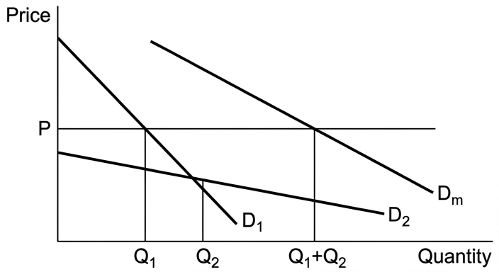
The diagram shows two individual demand curves, D1 and D2, each derived from diminishing marginal utility. They are downward sloping. At a given price P, consumer 1 demands Q1, consumer 2 demands Q2. The market demand curve Dm is the horizontal addition: at price P, total quantity demanded is Q1 + Q2. This illustrates how the theory constructs the market demand curve.
Strengths of the Theory
The theory provides a logical microeconomic foundation for the law of demand. It is simple and intuitive. For many frequently purchased normal goods, it predicts consumer responses to price changes reasonably well. It forms the basis for more sophisticated demand analysis.
Limitations and Evaluation
However, the theory has significant limitations that reduce its adequacy for all goods. First, it assumes rationality: consumers have perfect knowledge and can calculate marginal utilities. In reality, consumers often rely on habits or heuristics. Behavioural economics shows systematic deviations from rationality. Second, the theory assumes cardinal utility—that utility can be measured and compared—whereas modern economics uses ordinal utility. Third, it does not incorporate income and substitution effects, so it cannot explain inferior goods, where demand falls as income rises, or Giffen goods, where demand rises with price. For such goods, the market demand curve derived from this theory would be inaccurate. Fourth, the theory assumes a two-good world and continuously divisible units. In reality, consumers choose among many goods, and many goods are indivisible (e.g., a car). The consumer does not buy fractions of a car but decides whether to buy one or none. The marginal utility analysis of discrete choices is more complicated and may not yield a smooth demand curve. Fifth, the theory does not account for advertising, brand loyalty, or social influences that affect demand.
Evaluation and Conclusion
Weighing these, the theory is adequate for many goods, especially frequently purchased normal goods where the assumptions approximately hold. It provides a clear and logical explanation of the negative slope of the demand curve and the derivation of market demand. However, it is not adequate for all goods because its restrictive assumptions do not hold in many real-world situations. For a complete explanation of the market demand curve for all goods and services, we need a more flexible framework that includes indifference curves, income and substitution effects, and behavioural factors. Therefore, while the marginal utility theory is a useful starting point, it does not provide an adequate explanation for all goods and services.
The diminishing marginal utility theory provides a logical derivation of the downward-sloping market demand curve for many normal goods, but its assumptions of rationality, perfect knowledge, and cardinal utility limit its adequacy for all goods, particularly inferior, durable, or indivisible goods; overall, it is a useful but incomplete model.
Background Concept
Utility is the satisfaction a consumer derives from consuming a good or service. Total utility is the overall satisfaction from a given quantity. Marginal utility (MU) is the change in total utility from consuming an additional unit. The law of diminishing marginal utility states that as consumption of a good increases, the marginal utility derived from each additional unit eventually falls. Given a fixed income, a rational consumer will allocate spending so that the marginal utility per pound (or dollar) spent is equal across all goods—this is the equi-marginal principle. For a single good, if we assume only that good is consumed, the consumer continues to buy until MU equals the price (since the marginal benefit of the last unit equals its marginal cost). As price falls, the consumer moves along the diminishing MU curve to a higher quantity, tracing out an inverse relationship between price and quantity demanded: the individual demand curve. The market demand curve is the horizontal sum of all individual demand curves at each price.
Understanding the Question
The question asks you to evaluate whether the diminishing marginal utility theory of demand provides an adequate explanation of the market demand curve for all goods and services. “Adequate” means sufficient or satisfactory. The command word “evaluate” requires you to consider both the strengths and weaknesses of the theory and reach a justified conclusion. You must include a diagram (as stated: “with the aid of a diagram”) and explain it fully. The diagram should illustrate how the market demand curve is derived from individual demand curves that are themselves based on diminishing marginal utility. The phrase “for all goods and services” is crucial: you need to consider whether the theory works equally well for normal goods, inferior goods, luxury goods, durable goods, and frequently versus infrequently purchased items. The top band for AO1/AO2 requires detailed knowledge, fully developed explanations, and accurate use of analytical tools. The top band for AO3 requires a justified conclusion with developed evaluative comments.
Approach
- Explain the theory: Define marginal utility, diminishing marginal utility, and the equi-marginal principle. Show how an individual demand curve is derived.
- Explain market demand: Describe how market demand is the horizontal sum of individual demands. Use the diagram to illustrate this process.
- Present the case that the theory IS adequate: It provides a logical microfoundation for the law of demand; for many normal goods, it works well; it is the basis for more advanced models.
- Present the counter-case (limitations): Discuss unrealistic assumptions (rationality, perfect knowledge, cardinal utility), inability to explain inferior and Giffen goods (due to missing income and substitution effects), inapplicability to indivisible goods (e.g., cars, fridges), and oversimplified two-good world. Also mention behavioural economics challenges.
- Evaluate: Weigh the two sides. On balance, the theory is a useful simplification but not fully adequate for all goods. Conclude by stating that while it provides a good starting point, a more comprehensive model is needed for a complete explanation.
Step-by-Step Reasoning
Step 1: Explaining the theory.
A consumer gets utility from consuming good X. The MU of X diminishes as consumption increases. The consumer has a fixed income. To maximise utility, the consumer should consume up to the point where MUx = Px (assuming only X is consumed, or the equi-marginal condition holds across goods). If the price of X falls, the consumer can increase consumption until MUx falls to the level of the new price. This gives a negative relationship between price and quantity: a downward-sloping demand curve. This is a valid logical deduction under the assumptions.
Step 2: From individual to market demand.
The market demand curve is the sum of all individual demand curves. For each price, add up the quantities demanded by all consumers. The result is also downward sloping. The diagram shows two individual demand curves and the market demand curve as the horizontal sum. This part of the explanation is straightforward and the diagram helps visualise it.
Step 3: Strengths of the theory.
The theory is simple and intuitive. It explains why demand curves slope downward for most goods. It has predictive power for everyday goods like chocolate bars or petrol. It also provides the foundation for understanding consumer surplus and welfare effects. Therefore, for many goods, it is adequate.
Step 4: Limitations.
- Rationality: Consumers are assumed to have perfect knowledge of their preferences and market prices, and to always make utility-maximising choices. In reality, information is costly, and consumers use rules of thumb or are influenced by advertising. Behavioural economists like Kahneman and Tversky show that people systematically make decisions that violate rationality. This weakens the theory’s explanation of actual demand.
- Cardinal utility: The theory assumes utility is measurable and comparable across consumers. Modern economics treats utility as ordinal—only rankings matter. This does not invalidate the theory entirely, but it limits its claim to provide a complete explanation.
- Income and substitution effects: The theory focuses solely on the substitution effect via MU = P. It ignores that a price change also changes real income. For normal goods, the income effect reinforces the substitution effect, so the demand curve still slopes downward. But for inferior goods, the income effect works in the opposite direction; for Giffen goods, it is so strong that demand slopes upward. The marginal utility theory cannot capture this, so it fails to explain the market demand for inferior and Giffen goods. Since these goods exist (though rare), the theory is not adequate for “all goods and services.”
- Indivisible and durable goods: The theory assumes goods are consumed in infinitesimally small units. But many goods (cars, washing machines) are purchased as discrete units, and the consumer decides whether to buy one or none. The marginal utility of a single car is a step function, not a smooth declining curve. The market demand curve may still be downward sloping, but the derivation using MU = P is awkward. Similarly, for durable goods, utility is derived from the service flow over time, not from the good itself in a single period.
- Two-good world: The equi-marginal principle is typically taught with only two goods. In reality, consumers choose among thousands. While the principle can be extended, the complexity makes the simple model less adequate as an explanation.
- Ignoring other factors: Advertising, brand loyalty, habits, and social norms affect demand. The theory cannot incorporate these.
Step 5: Evaluation and conclusion.
Weigh the strengths and weaknesses. The theory scores well on simplicity and applicability to a wide range of goods. However, its restrictive assumptions mean it is not universally applicable. A justified conclusion would be that it provides an adequate explanation for many normal goods, especially frequently purchased ones, but not for all goods. To claim adequacy for all goods and services, one would need to ignore important exceptions. Therefore, the theory is a useful but incomplete model; a more complete explanation requires indifference curve analysis (which incorporates income and substitution effects) and behavioural economics.
Key Takeaways
- The marginal utility theory is one of the earliest formal models of consumer demand and successfully derives the downward-sloping demand curve.
- The market demand curve is the horizontal sum of individual demand curves.
- The theory’s assumptions (rationality, perfect knowledge, cardinal utility, divisibility) are strong and often violated in reality.
- It fails to explain the demand for inferior and Giffen goods because it lacks income effects.
- It is less suited to goods that are purchased infrequently or are indivisible.
- Evaluating a theory involves assessing both its logical coherence and its empirical applicability; a theory can be logically sound yet inadequate for real-world complexity.
- For top marks, you must include a fully explained diagram and reach a justified conclusion.
Common Mistakes
- Omitting the diagram or not explaining it: The question explicitly requires a diagram. You must refer to it in your answer and explain what it shows. A diagram alone without explanation will not earn the top band.
- Focusing only on individual demand without explaining market demand: The question is specifically about the market demand curve; you must show how the theory leads to the market curve.
- Providing a one-sided argument: Evaluation requires discussing both strengths and weaknesses. A purely positive or purely critical essay cannot score high evaluation marks.
- No justified conclusion: You must state whether the theory is adequate and why. A summary of points without a clear judgement is insufficient.
- Using too much jargon without developing the reasoning: Every chain of reasoning must be fully developed. Just stating that the theory assumes rationality is not enough; explain how that assumption affects adequacy.
- Confusing total and marginal utility: Ensure definitions are precise.
Things to Be Careful About
- Label your diagram clearly: axes (Price, Quantity), curves (D1, D2, Dm), and points (P, Q1, Q2, Q1+Q2).
- The diagram should be integrated into the essay, not an afterthought. Explain it immediately after presenting it.
- Use the phrase “market demand curve” repeatedly to stay focused on the question.
- When discussing limitations, relate each back to the adequacy of the market demand curve.
- For the conclusion, avoid fence-sitting. You can say the theory is adequate under certain conditions but overall not sufficient for all goods. That is a justified position.
- Ensure you define key terms like diminishing marginal utility, equi-marginal principle, and horizontal summation.
- Keep the essay organised: have clear paragraphs for each section (theory, strengths, limitations, evaluation, conclusion). The top band rewards logical coherence.
Subnormal and supernormal profits are only experienced in the short run and only by firms in perfect competition.
With the help of diagrams, evaluate this statement.
Introduction
This statement makes two claims: that subnormal and supernormal profits are only experienced in the short run, and that they are only experienced by firms in perfect competition. Both claims are incorrect. The analysis below shows that while perfect competition does indeed eliminate both types of profit in the long run, firms in imperfectly competitive market structures can sustain supernormal profits over the long run, and subnormal profits can also persist under certain conditions.
The case for the statement: perfect competition
In perfect competition, firms are price takers with a perfectly elastic demand curve (AR = MR = price). In the short run, a firm can earn supernormal profit if its average revenue exceeds its average total cost at the profit-maximising output (MC = MR). This is shown in the first diagram: the firm produces at Q1 where MC = MR, and the rectangle between AR and AC at that output represents supernormal profit. Alternatively, if AR lies below AC, the firm makes a subnormal loss.
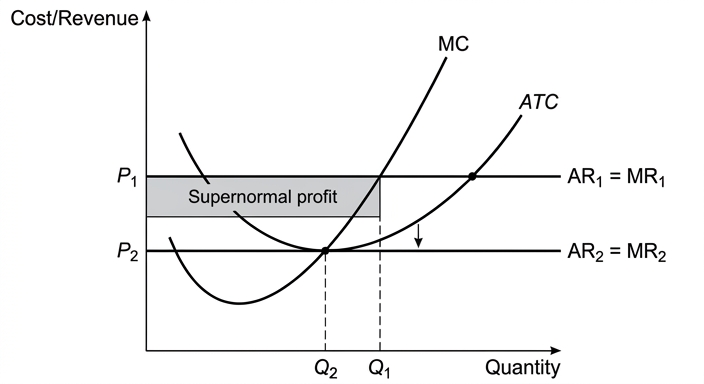
However, in the long run, the absence of barriers to entry and exit means that supernormal profit attracts new firms into the industry. This shifts the market supply curve rightwards, reducing the market price and therefore the firm's AR curve downwards until it is tangent to the AC curve at the minimum point of the AC curve. At this point, the firm earns only normal profit (AR = AC). Similarly, subnormal losses cause firms to exit, shifting supply leftwards, raising price until normal profit is restored. Thus, in perfect competition, subnormal and supernormal profits are indeed only short-run phenomena.
The case against the statement: imperfect competition
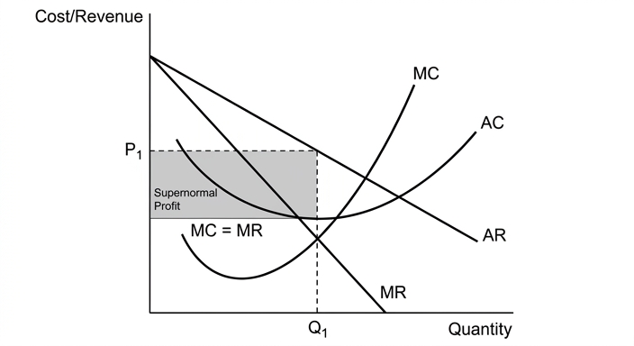
In monopoly, high barriers to entry (e.g. patents, economies of scale, legal restrictions) prevent new firms from entering the industry. A profit-maximising monopolist produces where MC = MR and sets price on the AR curve above that output. Because entry is blocked, the supernormal profit rectangle (AR - AC at Q1) persists in the long run. The monopolist does not experience subnormal profit in the long run because it can adjust its scale of production to avoid losses, and if demand is insufficient to cover average cost at any output, it will simply shut down.
In monopolistic competition, there is free entry and exit, so the short-run situation is similar to perfect competition: supernormal profit attracts new firms, and subnormal losses cause exit. In the long run, the firm's demand curve shifts until it is tangent to the AC curve, yielding only normal profit. So in this market structure, the statement's first claim (short run only) holds, but the second claim (only perfect competition) does not, because monopolistically competitive firms also experience these profits in the short run.
In oligopoly, the outcome is more complex. If firms collude (e.g. form a cartel), they can behave like a monopolist and earn long-run supernormal profit. If they compete aggressively (e.g. price wars), they may earn only normal profit or even subnormal profit in the short run. In the long run, barriers to entry (e.g. brand loyalty, huge capital requirements) can allow supernormal profit to persist, but intense rivalry can also erode it. Thus, both subnormal and supernormal profits can exist in both the short run and the long run, depending on the degree of collusion and the height of entry barriers.
Evaluation
The statement is false in two respects. First, subnormal and supernormal profits are not exclusive to perfect competition; they occur in all market structures in the short run. Second, they are not limited to the short run in all market structures: monopoly and collusive oligopoly can sustain supernormal profit in the long run, and subnormal profit can persist in oligopoly if firms are locked into a price war or if demand falls permanently and exit is costly. The only market structure where the statement's first claim holds is perfect competition (and monopolistic competition for the short-run-only claim), but even there the second claim is false because monopolistic competition also exhibits the same pattern.
Conclusion
The statement is largely incorrect. Subnormal and supernormal profits are experienced by firms in all market structures in the short run, and in imperfectly competitive markets — particularly monopoly and collusive oligopoly — supernormal profits can persist in the long run. The statement is only accurate for perfect competition, and even then it ignores the fact that other market structures also experience these profits in the short run.
The statement is largely incorrect: subnormal and supernormal profits are experienced by firms in all market structures in the short run, and in imperfectly competitive markets — particularly monopoly and collusive oligopoly — supernormal profits can persist in the long run. The statement is only accurate for perfect competition, and even then it ignores the fact that other market structures also experience these profits in the short run.
Background Concept
This question tests your understanding of profit types (normal, subnormal, supernormal) and how they behave over time (short run vs long run) across different market structures.
Normal profit is the minimum profit required to keep a firm in the industry in the long run. It is the opportunity cost of the entrepreneur's own resources and is included in the firm's average total cost (AC) curve. When a firm earns normal profit, total revenue equals total cost (including opportunity cost), so AR = AC.
Supernormal profit (also called abnormal or economic profit) is any profit above normal profit. It occurs when AR > AC at the profit-maximising output. It acts as a signal to attract new firms into the industry.
Subnormal profit (or loss) occurs when AR < AC at the profit-maximising output. The firm is earning less than normal profit and may exit the industry in the long run if the loss persists.
The short run is a period in which at least one factor of production is fixed (typically capital). Firms can vary output by changing variable factors (labour, raw materials) but cannot enter or exit the industry.
The long run is a period in which all factors are variable. Firms can enter or exit the industry, and existing firms can adjust their scale of production.
The key distinction between market structures is the degree of competition and the height of barriers to entry. Perfect competition has zero barriers to entry, so any supernormal profit is competed away in the long run. Monopoly has high barriers, so supernormal profit can persist. Monopolistic competition has free entry, so supernormal profit is competed away. Oligopoly sits in between, with outcomes depending on the behaviour of firms (collusion vs competition).
Understanding the Question
The question presents a statement with two distinct claims:
- "Subnormal and supernormal profits are only experienced in the short run" — meaning they never occur in the long run.
- "...and only by firms in perfect competition" — meaning no other market structure experiences these profits.
The command word is "evaluate", which requires you to assess the truth of the statement by examining both sides of the argument and reaching a justified conclusion. The question also explicitly requires diagrams ("With the help of diagrams"), so you must include at least one diagram and explain it fully. The mark scheme allocates 14 marks for AO1/AO2 (knowledge, understanding, and analysis) and 6 marks for AO3 (evaluation). The top band for AO1/AO2 requires "detailed knowledge and understanding", "fully developed explanations", and diagrams that are "fully explained". The top band for AO3 requires a "justified conclusion or judgement that addresses the specific requirements of the question" with "developed, reasoned and well-supported evaluative comment(s)".
The statement contains an absolute ("only"), which is a strong signal that the counter-case is the heart of the essay. You must show that the statement is false by providing counter-examples from other market structures.
Approach
The essay should be structured as follows:
-
Introduction: Define key terms (short run, long run, normal, subnormal, supernormal profit) and state the two claims to be evaluated. Give a brief preview of the conclusion.
-
First side — the case for the statement: Show that in perfect competition, the statement holds. Use a diagram to illustrate short-run supernormal profit and explain how entry eliminates it in the long run. Also explain the same for subnormal profit (exit eliminates it). This demonstrates that you understand the theory the statement is based on.
-
Second side — the case against the statement: This is the core of the evaluation. You need to show that:
- Monopoly can sustain supernormal profit in the long run (use a second diagram).
- Monopolistic competition also experiences subnormal and supernormal profits in the short run (so the statement's second claim is false).
- Oligopoly can have both types of profit in both time periods, depending on collusion and entry barriers.
-
Evaluation: Weigh the evidence. The statement is false on both counts, but it is partially true for perfect competition. The key criterion is the presence or absence of barriers to entry. Where barriers exist, supernormal profit can persist. Where they do not, it is competed away.
-
Conclusion: A clear, justified judgement that answers the question directly.
Step-by-Step Reasoning
Step 1: Define the key terms
- Short run: At least one factor is fixed. Firms can change output but cannot enter or exit.
- Long run: All factors are variable. Firms can enter or exit.
- Normal profit: The minimum profit to keep the firm in the industry; included in AC.
- Supernormal profit: Profit above normal profit (AR > AC).
- Subnormal profit: Profit below normal profit (AR < AC).
Step 2: Analyse perfect competition (the case for the statement)
In perfect competition:
- Many buyers and sellers, homogeneous product, perfect information, no barriers to entry or exit.
- The firm is a price taker, so its demand curve (AR = MR) is perfectly elastic at the market price.
- In the short run, the firm produces where MC = MR. If the market price is above the firm's AC at that output, the firm earns supernormal profit. If the price is below AC, it makes a subnormal loss.
- In the long run, supernormal profit attracts new firms. Entry shifts the market supply curve rightwards, reducing the market price. This continues until the firm's AR curve is tangent to its AC curve at the minimum point of AC. At this point, AR = AC, so only normal profit is earned. Similarly, subnormal losses cause firms to exit, shifting supply leftwards, raising price until normal profit is restored.
- Conclusion for perfect competition: The statement's first claim (short run only) is true for this market structure.
Step 3: Analyse monopoly (the case against the statement)
In monopoly:
- One firm, high barriers to entry (e.g. patents, economies of scale, legal restrictions).
- The firm is a price maker, facing a downward-sloping demand curve (AR). MR lies below AR.
- The profit-maximising output is where MC = MR. The price is set on the AR curve above that output.
- Because barriers to entry prevent new firms from entering, the supernormal profit (AR - AC at Q1) persists in the long run. The monopolist does not experience subnormal profit in the long run because it can adjust its scale or shut down if demand is insufficient.
- Conclusion for monopoly: The statement's first claim is false — supernormal profit can exist in the long run. The second claim is also false — monopoly experiences supernormal profit.
Step 4: Analyse monopolistic competition (further evidence against the statement)
In monopolistic competition:
- Many firms, differentiated products, free entry and exit.
- In the short run, a firm can earn supernormal profit if its differentiated product is popular (AR > AC at MC = MR). It can also make subnormal losses if demand is weak.
- In the long run, supernormal profit attracts new firms offering close substitutes. This shifts the firm's demand curve leftwards until it is tangent to the AC curve, yielding only normal profit. Subnormal losses cause exit, shifting the demand curve rightwards until normal profit is restored.
- Conclusion for monopolistic competition: The statement's first claim (short run only) is true for this market structure, but the second claim (only perfect competition) is false — monopolistic competition also experiences these profits in the short run.
Step 5: Analyse oligopoly (the most complex case)
In oligopoly:
- Few firms, high barriers to entry, interdependence between firms.
- If firms collude (e.g. form a cartel), they can behave like a monopolist and earn long-run supernormal profit. If they compete aggressively (e.g. price wars), they may earn only normal profit or even subnormal profit in the short run.
- In the long run, barriers to entry can allow supernormal profit to persist, but intense rivalry can erode it. Subnormal profit can persist if firms are locked into a price war or if demand falls permanently and exit is costly (e.g. due to sunk costs).
- Conclusion for oligopoly: Both claims of the statement can be false — subnormal and supernormal profits can exist in both the short run and the long run, depending on the degree of collusion and the height of entry barriers.
Step 6: Evaluation and conclusion
- The statement is false on both counts.
- The first claim (short run only) is true only for perfect competition and monopolistic competition, but false for monopoly and oligopoly.
- The second claim (only perfect competition) is false because all market structures experience these profits in the short run, and monopoly and oligopoly can experience them in the long run.
- The key determinant is the presence of barriers to entry. Where barriers are high (monopoly, collusive oligopoly), supernormal profit can persist. Where barriers are low or absent (perfect competition, monopolistic competition), it is competed away.
- The conclusion should state that the statement is largely incorrect, with the only element of truth being that in perfectly competitive markets, these profits are indeed short-run phenomena.
Key Takeaways
- Subnormal and supernormal profits are not unique to any single market structure; they occur in all market structures in the short run.
- The long-run persistence of supernormal profit depends on the height of barriers to entry. High barriers (monopoly, collusive oligopoly) allow it to persist; low barriers (perfect competition, monopolistic competition) cause it to be competed away.
- Subnormal profit can persist in the long run if exit is costly or if firms are locked into a price war (oligopoly).
- When evaluating a statement containing an absolute ("only", "always", "never"), the counter-case is the heart of the essay. You must provide examples that disprove the absolute.
- Diagrams are essential when the question explicitly requires them. They must be fully explained in the prose, not just drawn.
Common Mistakes
- One-sided answer: Writing only about perfect competition and ignoring other market structures. This would score zero for evaluation (AO3) because the question requires evaluation of the statement, which demands a two-sided treatment.
- No conclusion or a vague conclusion: The top band for AO3 requires a "justified conclusion or judgement that addresses the specific requirements of the question". A summary of both sides without a verdict is not enough.
- Omitting diagrams or not explaining them: The question explicitly says "With the help of diagrams". The mark scheme caps at Level 2 if no diagram is included. Even if a diagram is drawn, it must be fully explained in the prose — an unexplained diagram costs a band.
- Confusing short run and long run: The statement's first claim is about time periods. You must clearly distinguish between the two and explain how the profit situation changes as the time period changes.
- Confusing normal profit with zero profit: Normal profit is included in AC, so AR = AC means the firm is earning normal profit, not zero profit. This is a common error.
- Treating oligopoly as a single case: Oligopoly outcomes vary widely. You must acknowledge that collusion can lead to long-run supernormal profit, while competition can lead to normal or subnormal profit.
Things to Be Careful About
- Label every axis and curve on your diagrams: The mark scheme explicitly credits correct labelling. For the perfect competition diagram, label the axes (Quantity, Cost/Revenue), the curves (MC, AC, AR = MR), and the equilibrium points (P1, Q1). For the monopoly diagram, label AR, MR, MC, AC, and the profit-maximising output and price.
- Show the direction of shifts: In the perfect competition diagram, you may want to show how entry shifts the market supply curve and reduces the firm's AR. This demonstrates understanding of the long-run adjustment process.
- Use the extract's own evidence: This is not a data-response question, so there is no extract to use. However, you should use real-world examples where appropriate (e.g., Microsoft's long-run monopoly profits, the OPEC cartel's profits).
- Distinguish between short run and long run clearly: Use the definitions precisely. The short run is about fixed factors, not about a specific calendar time. The long run is about entry and exit.
- Reach a justified conclusion: Do not sit on the fence. The statement is largely false. State this clearly and explain why, referencing the evidence from each market structure.
A country imposes a tariff of 20% on imported goods and restricts the number of immigrants entering the country.
Evaluate, with the aid of a diagram(s), the impact of these two policies on the rate of inflation in that country.
Introduction
A tariff is a tax on imports, here 20%, which raises the domestic price of imported goods and imported raw materials. Restricting immigration reduces the supply of labour, tending to increase wages. Both policies are supply-side shocks that affect the short-run aggregate supply (SRAS) curve and, through it, the price level. This essay analyses the cost-push inflation effects and evaluates the conditions under which they may be offset by demand-side forces.
Impact of the tariff on inflation
The immediate effect of the tariff is to raise the price of imported consumer goods, directly increasing the consumer price index. More importantly, the tariff raises the cost of imported intermediate goods and raw materials for domestic producers. Higher input costs increase firms' costs of production, shifting the SRAS curve to the left. For a given aggregate demand (AD), this reduction in aggregate supply raises the average price level – cost-push inflation. The extent of the price rise depends on the price elasticity of demand for imported inputs and the ability of firms to pass on higher costs.
Impact of immigration restriction on inflation
Immigration expands the labour supply, moderating wage growth. Restricting immigration reduces the inflow of workers, particularly in labour-intensive sectors. This decreases the supply of labour, shifting the labour supply curve leftwards and raising the equilibrium wage rate. Higher wages are a key cost for firms, further increasing production costs and thus shifting SRAS leftwards again. The effect is stronger in labour-intensive industries where wages are a large share of total costs.
Diagram
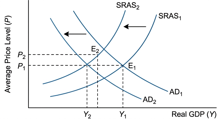
The combined effect of these two policies can be illustrated using an AD/AS diagram. Initially, the economy is at equilibrium E1, with price level P1 and real output Y1. The tariff and immigration restriction shift SRAS leftwards from SRAS1 to SRAS2 (due to higher import costs and higher wages). Meanwhile, the reduction in the number of immigrants reduces total consumption, investment, and government revenue, shifting AD leftwards from AD1 to AD2. The new equilibrium E2, at the intersection of AD2 and SRAS2, shows a higher price level P2 and lower output Y2. This indicates that, in this typical scenario, the cost-push effect dominates the demand-side contraction, resulting in higher inflation.
Evaluation
The net effect on inflation is not as straightforward as the simple cost-push story. Several factors moderate or offset the inflationary impact.
First, the leftward shift in AD from lower immigration exerts downward pressure on the price level. If the AD shift is large relative to the SRAS shift, the price level could even fall. The outcome depends on the marginal propensity to consume of immigrants and the overall size of the immigrant population.
Second, the elasticity of supply of domestically produced goods matters. If domestic firms can easily expand output to replace imports made dearer by the tariff, the upward pressure on prices is limited. In the short run, however, domestic supply is often inelastic, so price increases are more likely.
Third, the availability of domestic labour is crucial. If there is significant domestic unemployment, firms may hire local workers without substantially raising wages, dampening the wage-push effect. Conversely, if labour markets are already tight, the immigration restriction will cause sharper wage rises.
Fourth, the tariff may encourage domestic investment in import-competing industries, eventually increasing aggregate supply. However, this effect takes time and is uncertain.
Finally, the policies operate with different time lags: the tariff's price impact is immediate, while wage and AD effects unfold gradually. In the short run, inflation is more likely to increase; in the long run, adjustments in labour and product markets could mitigate the rise.
Conclusion
Overall, both the tariff and the immigration restriction are likely to increase the rate of inflation in the short run by raising production costs and shifting SRAS leftwards. However, the net increase depends critically on the accompanying reduction in aggregate demand from lower immigration, the elasticities of domestic supply and labour supply, and the time horizon. Given that the tariff directly raises prices and that labour markets are often tight in the short run, a moderate rise in inflation is the most plausible outcome, but the magnitude is ambiguous without empirical evidence on specific elasticities and the state of the economy.
The two policies are likely to increase inflation in the short run due to cost-push effects, but the net impact is moderated by demand-side reductions and the responses of domestic supply and labour markets; the final effect is ambiguous in magnitude and depends on elasticities and time horizon.
Background Concept
Inflation is a sustained increase in the general price level. It can be caused by demand-pull factors (excess aggregate demand) or cost-push factors (rising costs of production). A tariff is a tax on imports; it directly raises the price of imported goods and also raises the cost of imported raw materials and intermediate goods for domestic producers. Immigration restriction reduces the supply of labour, which tends to increase wages as firms compete for a smaller pool of workers. Both policies increase firms' costs – input costs and wage costs – which shifts the short-run aggregate supply (SRAS) curve to the left, generating cost-push inflation. However, immigration also reduces aggregate demand (fewer consumers, workers, and entrepreneurs), shifting the AD curve leftwards, which puts downward pressure on prices. The net effect on inflation depends on the relative magnitudes of these two shifts and on elasticities.
Understanding the Question
You are asked to evaluate the impact of two specific policies on the rate of inflation. The command word 'evaluate' requires you to consider both sides – not only the inflationary forces but also factors that could reduce or reverse the inflation, and then reach a justified conclusion. 'With the aid of a diagram(s)' means you must include at least one diagram (here an AD/AS diagram) and fully explain it in the text – a diagram alone without explanation loses marks. The question is worth 20 marks and is levels-marked: the top band requires detailed knowledge, developed analysis, a fully explained diagram, and a justified conclusion. You must address both policies in sufficient depth; treating only the tariff or only immigration restriction will cap your marks.
Approach
- Define and explain the two policies and how each could cause cost-push inflation.
- Use an AD/AS diagram to show the leftward shift in SRAS from both policies and the leftward shift in AD from reduced immigration. Explain the diagram step by step.
- Evaluate the net impact by considering:
- The relative size of the AD shift vs the SRAS shift.
- Elasticities of domestic supply and labour supply.
- The state of the domestic labour market (slack vs tight).
- Time lags (short run vs long run).
- Possible long-run supply-side benefits (domestic investment).
- Reach a justified conclusion that answers the question directly, stating the most likely outcome and under what conditions it would differ.
Step-by-Step Reasoning
Step 1: Tariff and cost-push inflation
- A 20% tariff increases the domestic price of imported consumer goods. This directly raises the CPI (measured inflation).
- Many firms use imported raw materials and components (e.g., steel, electronics). The tariff raises these input costs, so firms' average and marginal costs rise.
- Firms respond by reducing output at any given price level, i.e., SRAS shifts left. For a fixed AD, the price level rises and output falls – classic cost-push inflation.
- The size of the price increase depends on the proportion of imported inputs in production and the price elasticity of demand for those inputs; if demand is inelastic, cost increases are more easily passed on.
Step 2: Immigration restriction and cost-push inflation
- Immigration increases the supply of labour, which helps keep wages low. Restricting immigration reduces the growth of the labour force, especially in industries that rely on immigrant labour (agriculture, construction, hospitality).
- The labour supply curve shifts left, so the equilibrium wage rises. Higher wages are a cost of production, so SRAS shifts left again.
- The effect is larger where labour costs are a high proportion of total costs and where immigrant labour is a significant share of employment.
Step 3: The AD/AS diagram
- Draw an AD/AS diagram with the average price level (P) on the vertical axis and real GDP (Y) on the horizontal axis.
- Draw initial AD1 and SRAS1 intersecting at E1 (P1, Y1).
- Show SRAS shifting leftwards to SRAS2 (due to tariff and wage increases). Also show AD shifting leftwards to AD2 (due to reduced consumption and investment from fewer immigrants).
- The new equilibrium E2 is at the intersection of AD2 and SRAS2. In the typical case where the SRAS shift dominates, P2 > P1 (inflation) and Y2 < Y1 (recession).
- Explain that if the AD shift were larger, P could fall; the relative shift is an empirical question.
- Label all curves, axes, and equilibrium points clearly.
Step 4: Evaluation of the net impact
- Demand-side offset: Immigrants are also consumers; fewer immigrants means lower consumption and possibly lower investment (fewer entrepreneurs, lower housing demand). This reduces AD, which lowers the price level. The net change in the price level depends on whether the leftward shift in AD is larger or smaller than the leftward shift in SRAS.
- Elasticity of domestic supply: If domestic firms can quickly increase production of goods previously imported, the upward price pressure from the tariff is muted. But in the short run, domestic supply is often inelastic due to capacity constraints, so prices rise.
- Availability of domestic labour: If there is significant unemployment, firms can replace immigrant labour with domestic workers without raising wages much. In a full-employment economy, the wage increase will be larger.
- Time horizon: In the short run, the tariff's price effect is immediate, and wages adjust slowly, so cost-push inflation is more pronounced. Over time, the economy may adjust: domestic firms may invest to replace imports (increasing AS), and workers may move between sectors. The long-run impact could be lower.
- Potential long-run AS increase: The tariff might protect domestic industries and encourage import-substituting investment, which could eventually increase AS. However, this is uncertain and takes time. It could even reduce productivity if it shelters inefficient firms.
Step 5: Conclusion
- The most plausible short-run outcome is a moderate increase in inflation because the cost-push effects are immediate and direct, while the demand-side offset takes longer to materialise and may be smaller in magnitude unless immigration is very large.
- However, if the economy is in a deep recession with high unemployment, the wage-push effect may be weak, and the AD contraction could even cause deflation.
- Therefore, a justified conclusion is that inflation is likely to rise, but the magnitude is ambiguous and depends critically on the elasticities and the state of the economy at the time.
Key Takeaways
- Tariffs and immigration restrictions are supply-side policies that can cause cost-push inflation.
- Both policies shift SRAS left, but immigration restriction also reduces AD, creating an offsetting effect on the price level.
- A fully explained AD/AS diagram is essential to show both shifts and the resulting change in price level and output.
- Evaluation must consider elasticities, time lags, the state of the labour market, and potential long-run adjustments.
- A justified conclusion must weigh the opposing forces, not just summarise.
Common Mistakes
- One-sided answer: Discussing only cost-push inflation without considering the demand-side effects of immigration restriction or the possibility of demand-pull offset. This loses all evaluation marks.
- No diagram or incomplete diagram: Omitting the AD/AS diagram or drawing it without labels and explanation. The top band requires diagrams to be fully explained.
- Confusing cost-push and demand-pull: For example, stating that the tariff increases demand (it does not; it reduces imports but may not increase total AD).
- Treating the two policies separately without synthesis: The question asks for the combined impact; but it is acceptable to analyse each separately and then combine. Failing to mention one policy entirely is a major omission.
- Vague conclusion: Saying 'it depends' without specifying on what and under which conditions the outcome differs. A top-band conclusion must provide a clear judgement.
- Ignoring the diagram in the prose: Inserting a diagram reference but not explaining what it shows in the text. The explanation must be part of the essay.
Things to Be Careful About
- Use the exact tariff percentage: The question specifies 20% – mention it, but you don't need to calculate its exact price impact.
- Distinguish short run and long run: The inflationary impact is different in different time frames.
- Label the diagram correctly: Axes (Price Level, Real GDP), curves (SRAS1, SRAS2, AD1, AD2), equilibrium points (E1, E2), and arrows for shifts.
- Do not assume the tariff automatically reduces demand: It may reduce imports but also may crowd out domestic consumption of other goods; the net AD effect is ambiguous. The more clear-cut demand effect comes from immigration reduction.
- Use correct terminology: 'cost-push inflation', 'aggregate supply', 'wage-push', 'elasticity of supply'.
- Stay focused on inflation: Do not drift into discussing the balance of payments or current account deficit unless it directly links to inflation (e.g., exchange rate pass-through).
- Structure the essay logically: Use clear sections (Introduction, Analysis, Diagram, Evaluation, Conclusion). This helps the examiner see the structure and rewards organisation.
Evaluate whether an increase in a government's budget deficit will always lead to economic growth.
Introduction
A budget deficit occurs when government spending exceeds tax revenue in a given period. Economic growth refers to an increase in real GDP, either actual (short-run) or potential (long-run). This essay evaluates whether an increase in the deficit always leads to growth.
The case that a budget deficit can lead to economic growth
An increase in the budget deficit, typically financed by borrowing, raises government spending (G) without an immediate rise in taxes. This directly increases aggregate demand (AD = C + I + G + X – M). The rise in G shifts the AD curve to the right.
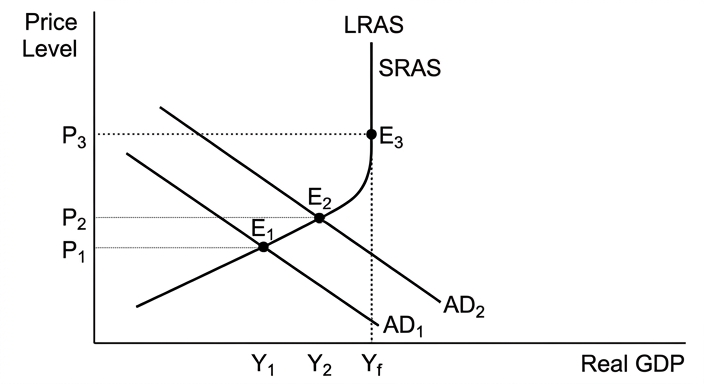
In the diagram, the economy initially at Y1 with AD1 and SRAS. An increase in G shifts AD to AD2. If the economy is operating below full employment (with a negative output gap), the increase in AD raises real output from Y1 to Y2, with only a modest rise in the price level from P1 to P2. This is actual economic growth. The multiplier effect amplifies the initial spending: the increase in income leads to higher consumption, further boosting AD. The size of the multiplier depends on the marginal propensities to consume, tax, and import. A larger multiplier produces a greater final increase in national income.
Furthermore, if the deficit-financed spending is directed towards infrastructure, education, or R&D, it can increase the economy's productive capacity, shifting LRAS to the right and generating potential (long-run) growth. This supply-side effect can sustain growth without inflationary pressure.
The case against – why a budget deficit may not always lead to growth
First, crowding out may occur. To finance the deficit, the government borrows from the loanable funds market, raising interest rates. Higher interest rates reduce private investment (I) and consumption of durable goods, offsetting the initial increase in G. If crowding out is complete, AD may not rise at all, and growth fails to materialise.
Second, if the economy is already at or near full employment (positive output gap), the increase in AD will mainly cause demand-pull inflation rather than a rise in real output. In the diagram, if the economy is on the vertical portion of the SRAS (or at full capacity), the shift from AD1 to AD2 raises the price level to P3 but output remains at Yf. Inflation may also erode international competitiveness, worsening the current account and reducing net exports, further dampening growth.
Third, the deficit may be financed by printing money (monetisation), leading to inflation and potentially hyperinflation if expectations become unanchored. High inflation discourages investment and long-term planning, harming growth.
Fourth, the effectiveness of the deficit depends on expectations. If households and firms anticipate future tax rises to repay the debt, they may increase saving (Ricardian equivalence), reducing the multiplier effect. Consumer confidence may fall, offsetting the stimulus.
Fifth, the deficit may be used for current consumption rather than investment, providing only a temporary boost to AD with no lasting effect on potential output. Once the spending ends, growth may stall.
Evaluation
The impact of a budget deficit on growth depends critically on the state of the economy. In a recession with high unemployment and spare capacity, the deficit is likely to stimulate actual growth with minimal inflation. The multiplier is larger when leakages (saving, imports, taxes) are small. Conversely, at full employment, the deficit mainly causes inflation and crowding out, with no real growth. The composition of spending matters: supply-enhancing expenditure can generate long-run growth, while consumption spending only provides a short-run boost. The method of financing also matters: borrowing from the private sector may crowd out investment, while central bank financing may fuel inflation. Expectations and Ricardian equivalence can weaken the impact. The Phillips curve trade-off suggests that in the short run, lower unemployment (growth) comes at the cost of higher inflation, but in the long run, the natural rate of unemployment is independent of inflation.
Conclusion
A budget deficit does not always lead to economic growth. It can stimulate actual growth in the short run when the economy is below full employment and the multiplier is large, and it can promote potential growth if spent on productive capacity. However, crowding out, inflation, Ricardian equivalence, and the composition of spending can prevent or reverse growth. The statement is therefore not always true; the outcome depends on the economic context, the type of spending, and the method of finance.
A budget deficit can stimulate economic growth in the short run when the economy is below full employment and the multiplier is large, but it does not always lead to growth; it may cause crowding out, inflation, or worsen the current account, and long-run growth requires supply-side improvements. Therefore, the statement is not always true.
Background Concept
A budget deficit is the shortfall when government spending exceeds tax revenue. It is a form of expansionary fiscal policy. Economic growth is measured as the percentage increase in real GDP. There are two types: actual growth (short-run increases in output using existing capacity) and potential growth (long-run expansion of the economy's productive capacity). The AD/AS model is the standard tool to analyse the impact of fiscal policy on output and prices. The multiplier concept shows how an initial injection of spending leads to a larger final increase in national income through successive rounds of consumption. Crowding out refers to the reduction in private spending caused by higher interest rates or taxes resulting from government borrowing. Ricardian equivalence suggests that rational consumers anticipate future taxes and save more, offsetting the stimulus.
Understanding the Question
The question asks whether an increase in the government's budget deficit will always lead to economic growth. The word "always" makes this an absolute claim. To evaluate it, we must consider both the mechanisms through which a deficit could promote growth and the conditions under which it might fail to do so or even harm growth. The command word "Evaluate" requires a two-sided analysis and a justified conclusion. The top band demands detailed knowledge, developed analysis, and a well-supported evaluative judgement. The question does not specify short-run or long-run growth, so both should be considered.
Approach
- Define key terms: budget deficit, economic growth (actual and potential).
- Present the case for growth: use AD/AS diagram to show how increased G raises AD, leading to higher real output when there is spare capacity. Explain the multiplier effect. Mention supply-side spending that can increase LRAS.
- Present the case against: crowding out, inflation at full employment, Ricardian equivalence, composition of spending, financing methods, expectations.
- Evaluate: weigh the conditions under which each outcome is more likely. Use criteria such as the state of the economy (output gap), size of multiplier, type of spending, method of finance, and time horizon.
- Conclude with a justified judgement that answers the specific question: it does not always lead to growth.
Step-by-Step Reasoning
Step 1: Definitions
- Budget deficit: G > T. It increases the national debt.
- Economic growth: increase in real GDP. Short-run growth occurs when actual output rises towards potential; long-run growth occurs when potential output itself increases.
Step 2: The positive case
- An increase in G directly adds to AD. In the AD/AS model, AD shifts right.
- If the economy is in a recession (negative output gap), there is spare capacity. The SRAS curve is relatively elastic. The increase in AD raises real output significantly with little inflation. This is actual growth.
- The multiplier effect: the initial increase in G raises income, which leads to higher consumption (C), further increasing AD. The multiplier = 1/(1-MPC) in a simple closed economy. With taxes and imports, the multiplier is smaller but still >1.
- If the deficit is used for investment in infrastructure, education, or technology, it can increase the economy's productive capacity, shifting LRAS to the right. This generates potential growth, which can be sustained without inflation.
Step 3: The negative case (why it may not lead to growth)
- Crowding out: government borrowing increases demand for loanable funds, raising interest rates. Higher interest rates reduce private investment (I) and consumption of durable goods. If the fall in I exactly offsets the rise in G, AD does not change. Partial crowding out reduces the net stimulus.
- At full employment: if the economy is already at potential output, the SRAS is vertical (or steep). The increase in AD only raises the price level (inflation) with no increase in real output. Inflation may reduce real incomes and international competitiveness, potentially reducing net exports and future growth.
- Ricardian equivalence: if consumers anticipate that the deficit will be repaid by future taxes, they increase saving to pay those taxes, reducing current consumption. The offsetting fall in C neutralises the rise in G. Empirical evidence is mixed, but it weakens the multiplier.
- Composition of spending: if the deficit finances current consumption (e.g., public sector wages) rather than investment, it provides only a temporary boost. Once the spending ends, growth may revert. No lasting increase in potential output.
- Financing method: if the central bank monetises the deficit (prints money), it can lead to inflation. High inflation creates uncertainty, reduces investment, and can harm long-run growth. If the government borrows from abroad, it may lead to a current account deficit and future debt servicing problems.
- Expectations: if the deficit is seen as unsustainable, it may reduce business confidence and investment, offsetting the stimulus.
Step 4: Evaluation
- The key determinant is the state of the economy. In a deep recession with high unemployment and spare capacity, the deficit is likely to be effective in raising output with little inflation. The multiplier is larger because leakages (saving, imports) are smaller when income is low.
- At full employment, the deficit is likely to cause inflation and crowding out, with no real growth. The Phillips curve shows a short-run trade-off but no long-run trade-off; in the long run, the economy returns to the natural rate of unemployment.
- The size of the multiplier matters: a high MPC, low MPT, low MPM increase the multiplier. In a closed economy with low taxes, the multiplier is larger.
- The type of spending: supply-side spending can generate long-run growth, while consumption spending only provides a short-run boost. The effectiveness also depends on the efficiency of government projects.
- Time horizon: in the short run, a deficit can stimulate actual growth; in the long run, sustained growth requires increases in potential output. A deficit that crowds out private investment may reduce long-run growth even if it boosts short-run output.
- The method of finance: borrowing from the private sector may crowd out investment; borrowing from the central bank may cause inflation; borrowing from abroad may lead to future debt crises.
- Expectations and Ricardian equivalence: if consumers fully anticipate future taxes, the multiplier is zero. However, in practice, consumers may not fully adjust, especially if they are liquidity-constrained.
Step 5: Conclusion
The statement that a budget deficit will always lead to economic growth is false. It can lead to growth under specific conditions (spare capacity, large multiplier, productive spending), but it can also fail due to crowding out, inflation, Ricardian equivalence, or poor composition of spending. Therefore, the outcome is conditional, not guaranteed.
Key Takeaways
- A budget deficit is expansionary fiscal policy that increases AD.
- The effect on growth depends on the slope of AS (spare capacity vs full employment).
- The multiplier amplifies the initial spending but is reduced by leakages and crowding out.
- Crowding out, Ricardian equivalence, and inflation are key limitations.
- Long-run growth requires supply-side improvements, not just demand stimulus.
- Evaluation must consider the state of the economy, composition of spending, method of finance, and expectations.
- An absolute claim like "always" should be challenged with counterexamples.
Common Mistakes
- One-sided answer: only arguing that deficits cause growth or only that they don't. Must present both sides for evaluation marks.
- No diagram: the AD/AS diagram is essential to illustrate the effect and the conditions. Without it, the analysis is less developed.
- Confusing nominal and real growth: the deficit may increase nominal GDP but not real GDP if inflation is high.
- Ignoring the long run: focusing only on short-run demand effects without considering supply-side consequences or crowding out of investment.
- No conclusion or a vague conclusion: must provide a justified judgement that directly answers the question.
- Overgeneralising: assuming the multiplier is always large or that crowding out always occurs. Must discuss conditions.
- Misusing the multiplier: forgetting that the multiplier works through induced consumption and that leakages reduce its size.
- Not addressing the "always": the question specifically asks whether it will always lead to growth, so the answer must show that it does not always happen.
Things to Be Careful About
- Label axes and curves in the diagram: price level on vertical axis, real GDP on horizontal axis; AD1, AD2; SRAS; LRAS; equilibrium points.
- Explain the diagram in the text: state which curve shifts, why, and the effect on output and prices.
- Use economic terminology precisely: budget deficit, fiscal policy, aggregate demand, multiplier, crowding out, Ricardian equivalence, output gap, demand-pull inflation, potential output.
- Distinguish between short-run and long-run growth.
- When evaluating, use criteria such as the state of the economy, size of multiplier, type of spending, and time horizon.
- Ensure the conclusion is justified: state that it does not always lead to growth, and explain under what conditions it does or does not.
- Avoid fence-sitting: the conclusion should be clear, not "it depends" without specifying the conditions.