Economics 9708/43 — October/November 2025
Cambridge A-Level · A Level Data Response and Essays · worked solutions for every part, with the mark scheme
Topics Characteristics of Countries at Different Levels of Development · Equity, Poverty and Redistribution · Economic Development and Living Standards · Globalisation and Economic Integration · Relationships Between Countries at Different Levels of Development · Market Structures · +6 more
Inequality and globalisation
A government commission published a report saying that global poverty and inequality were worsening and there was a risk that the gap between the rich and the poor would increase.
But, according to a newspaper, a lot of what is said about inequality is wrong. It overlooks the fact that the past 50 years saw a period of dramatic reduction in global inequality. The normal measurement of relative inequality is the Gini coefficient. The figure for global inequality in 1975 was 0.75, in 2020 it was 0.72 and in 2022 it was 0.67.
It is important to understand this trend rather than make the mistake of the commission.
The fall in global inequality should not come as a surprise. For about two hundred years the benefits of industrialisation went mainly to countries in Europe and North America. Income inequality between these countries and poorer countries worsened. The spread of globalisation in recent decades has meant this difference has lessened. Countries such as China and India have benefited from large increases in per capita (average) income, as shown in Table 1.1.
Table 1.1 Per capita (average) income and Gini coefficient for China and India 1990 and 2016
| Per capita (average) income (US$) 1990 | Per capita (average) income (US$) 2016 | Gini coefficient 1990 | Gini coefficient 2016 | |
|---|---|---|---|---|
| China | <1000 | >13000 | 0.32 | 0.38 |
| India | <1200 | >7000 | 0.32 | 0.36 |
With such an increase in per capita incomes maybe some level of inequality does not matter. Indeed, it might be a necessary condition for economic growth. Instead of concentrating on eliminating inequality perhaps the focus should be on the absolute position of the poorest.
If the attention is on the relief of poverty rather than the wealth of the richest, improvements can be seen. Life expectancy has increased, most noticeably by ten years in the past two decades in the poorest region of sub-Saharan Africa. Literacy rates have also increased. Those in absolute poverty across the world have fallen from more than a third to under a tenth of the world's population. And all this while the world's population has increased.
Critics of globalisation and foreign direct investment (FDI) by multinational companies point to the possible negative environmental effects, the weakening of individual cultures and the reliance on international financial institutions that can fail. They also claim there can be exploitation of workers leading to greater wage inequality and possible increases in domestic unemployment as cheaper goods are imported.
Source: The Times, 23 August 2021
The article refers to the Gini coefficient. With the help of a diagram explain the link between a Gini coefficient and a Lorenz curve.
Answer
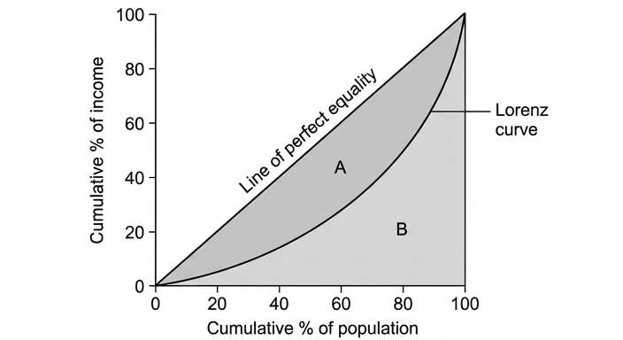
A Lorenz curve shows the cumulative percentage of income against the cumulative percentage of the population. The line of perfect equality is a 45-degree line from the origin. The Lorenz curve lies below it, showing the actual distribution of income. The further the Lorenz curve is from the line of perfect equality, the more unequal the distribution.
The Gini coefficient is calculated as:
Gini = Area A / (Area A + Area B)
where Area A is the area between the line of perfect equality and the Lorenz curve, and Area B is the area below the Lorenz curve.
The Gini coefficient measures the extent to which the distribution of income within a country is unequal. A value of 0 represents perfect equality (everyone has the same income). A value of 1 represents perfect inequality (one person has all the income).
The Gini coefficient is the ratio of the area between the Lorenz curve and the line of perfect equality to the total area under the line of perfect equality.
Background Concept
The Lorenz curve and the Gini coefficient are two closely related tools used to measure income or wealth inequality within a country. The Lorenz curve is a graphical representation of the distribution. The Gini coefficient is a numerical summary derived from that graph. Together, they provide a way to quantify and compare inequality across countries or over time.
Understanding the Question
This question asks you to explain the link between the Gini coefficient and a Lorenz curve, and to do so with the help of a diagram. The command word is 'explain', which means you need to define the terms and show how they relate to each other. The 'with the help of a diagram' instruction means a correctly drawn and labelled Lorenz curve diagram is required to earn full marks. The question is worth 5 marks, so the answer should be concise but complete, covering the diagram, the formula, and the interpretation of the coefficient's values.
Approach
- Draw and label the Lorenz curve diagram. This is the core of the answer. The axes must be labelled, the line of perfect equality must be drawn, and the Lorenz curve must be shown below it. The areas A and B should be identified.
- State the formula for the Gini coefficient. Show it as a ratio of areas on the diagram.
- Explain the meaning of the Gini coefficient. Define what a value of 0 and a value of 1 represent, and how the coefficient relates to the position of the Lorenz curve.
Step-by-Step Reasoning
- The Diagram: Start by drawing a square or a right-angled triangle. The horizontal axis (x-axis) should be labelled 'Cumulative percentage of population' (from 0% to 100%). The vertical axis (y-axis) should be labelled 'Cumulative percentage of income' (from 0% to 100%).
- The Line of Perfect Equality: Draw a 45-degree line from the bottom-left corner (0,0) to the top-right corner (100,100). This line represents a situation where every percentage of the population receives the same percentage of income. For example, the bottom 20% of the population receives 20% of the income, the bottom 50% receives 50%, and so on.
- The Lorenz Curve: Draw a curve that starts at (0,0) and ends at (100,100) but bows downwards away from the line of perfect equality. This curve shows the actual distribution. For example, it might show that the bottom 20% of the population receives only 5% of the total income.
- Labelling the Areas: The area between the line of perfect equality and the Lorenz curve is typically labelled 'A'. The area under the Lorenz curve (between the curve and the axes) is labelled 'B'. The total area under the line of perfect equality is A + B.
- The Formula: The Gini coefficient is calculated as A / (A + B). This formula directly links the numerical coefficient to the graphical representation. The larger the area A (the further the Lorenz curve is from the line of equality), the larger the Gini coefficient.
- Interpretation: A Gini coefficient of 0 means A = 0, so the Lorenz curve is the same as the line of perfect equality. A Gini coefficient of 1 means B = 0, so the Lorenz curve is as far away as possible, implying one person has all the income. In reality, most countries have a Gini coefficient between 0.25 and 0.60.
Key Takeaways
- The Lorenz curve is a visual tool; the Gini coefficient is a numerical summary.
- The Gini coefficient is derived directly from the Lorenz curve diagram.
- A higher Gini coefficient (closer to 1) indicates greater inequality.
- A lower Gini coefficient (closer to 0) indicates greater equality.
Common Mistakes
- Drawing the Lorenz curve above the line of perfect equality: This is impossible. The Lorenz curve must always be on or below the line of perfect equality.
- Not labelling the axes: The axes must be clearly labelled 'Cumulative % of population' and 'Cumulative % of income'. Unlabelled diagrams lose marks.
- Confusing the formula: The Gini coefficient is A/(A+B), not B/(A+B).
- Omitting the diagram: The question explicitly asks for a diagram. Omitting it will result in a maximum of 3 marks out of 5.
- Not explaining the meaning of 0 and 1: The mark scheme specifically awards marks for stating that 0 = perfect equality and 1 = perfect inequality.
Things to Be Careful About
- Ensure the Lorenz curve is drawn as a smooth curve, not a straight line or a series of straight segments.
- The diagram must be fully explained in the text. Do not just draw it and assume the examiner will understand. The text should describe what the diagram shows.
- The formula should be written clearly, even if it is just in words (e.g., 'Area A divided by the total area under the line of perfect equality').
Answer
Equality generally refers to equal opportunity or equal treatment for all individuals. It is a state where everyone has the same starting point or is treated the same way.
Equity refers to fairness and justice in outcomes. It recognises that different people may need different levels of support to achieve a fair outcome, and it may involve redistributing resources to correct for historical or structural disadvantages.
Equality is about sameness of opportunity or treatment; equity is about fairness of outcome.
Background Concept
In economics and public policy, 'equality' and 'equity' are often used interchangeably in everyday language, but they have distinct meanings. Understanding the difference is crucial for analysing policies related to taxation, welfare, and redistribution.
Understanding the Question
This is a straightforward 2-mark question asking you to 'distinguish between' equity and equality. This means you need to provide a clear definition of each term, highlighting the key difference between them. The answer should be concise and precise.
Approach
- Define 'equality' in the context of economics (equal opportunity/treatment).
- Define 'equity' in the context of economics (fairness of outcome).
- The distinction is that equality focuses on the process (sameness), while equity focuses on the result (fairness).
Step-by-Step Reasoning
- Equality: This concept is about uniformity. In an economic context, it often refers to equality of opportunity, meaning everyone should have the same chance to succeed, regardless of their background. It can also refer to equality of outcome, where everyone receives the same amount of income or wealth, but this is a more extreme interpretation. The standard economic definition leans towards equality of opportunity.
- Equity: This concept is about justice and fairness. It acknowledges that because people start from different positions (due to factors like family wealth, education, or discrimination), simply providing equal opportunity may not lead to a fair outcome. Equity, therefore, may require unequal treatment (e.g., higher taxes on the rich, targeted welfare for the poor) to achieve a more just distribution of resources.
- The Key Distinction: The core difference is that equality is about sameness, while equity is about fairness. A policy can be equal (everyone gets the same benefit) but inequitable (a rich person doesn't need it, a poor person does). Conversely, a policy can be equitable (giving more to those who need it) but unequal (not everyone receives the same amount).
Key Takeaways
- Equality = sameness of opportunity or treatment.
- Equity = fairness of outcome.
- These two concepts can conflict; a perfectly equal distribution may not be considered fair, and a fair distribution may not be equal.
Common Mistakes
- Using the terms interchangeably: This is the most common mistake. The question explicitly asks you to distinguish between them, so you must show you understand they are different.
- Providing only one definition: You must define both terms to earn both marks.
- Overcomplicating the answer: This is a 2-mark question. A short, clear sentence for each is sufficient.
Things to Be Careful About
- Be precise with your language. 'Equality' is about sameness; 'equity' is about fairness. Do not say 'equality is when everyone is equal' – this is circular. Instead, say 'equality refers to equal opportunity'.
“But, according to a newspaper, a lot of what is said about inequality is wrong.”
Analyse whether there is a conflict between what the newspaper wrote about changes in equality and Table 1.1.
Answer
There is no direct conflict between the newspaper's claim and Table 1.1, because they are measuring different things.
The newspaper reports that global inequality (measured by the Gini coefficient) has fallen from 0.75 in 1975 to 0.67 in 2022. This is a measure of inequality between all countries.
Table 1.1 shows the Gini coefficient for individual countries (China and India). It shows that within China, inequality has risen from 0.32 to 0.38, and within India, it has risen from 0.32 to 0.36.
These two trends are not contradictory. Globalisation can reduce inequality between countries (as poorer countries like China and India grow faster than richer ones) while simultaneously increasing inequality within those same countries (as some regions and workers benefit more than others).
Furthermore, both the newspaper and the table agree that per capita incomes in China and India have risen substantially, which is a key driver of the fall in global inequality.
There is no conflict; the newspaper refers to falling global inequality between countries, while Table 1.1 shows rising inequality within specific countries.
Background Concept
Inequality can be measured at different levels: global inequality (between all individuals in the world), between-country inequality (comparing average incomes of different countries), and within-country inequality (comparing incomes of individuals within a single country). These different measures can move in opposite directions. This is a key insight for understanding the effects of globalisation.
Understanding the Question
This is a 5-mark 'analyse' question. It presents a potential conflict: the newspaper says global inequality is falling, but Table 1.1 shows that the Gini coefficients for China and India (two major developing countries) have risen. The question asks you to analyse whether this is a genuine conflict. The command word 'analyse' requires you to break down the information, identify the different levels of measurement, and explain why the data is not contradictory.
Approach
- Identify what the newspaper is measuring: The newspaper cites a fall in the global Gini coefficient. This measures inequality between all people in the world, or between the average incomes of all countries.
- Identify what Table 1.1 is measuring: The table shows the Gini coefficient within China and within India. This measures domestic inequality.
- Explain why they can move in opposite directions: Globalisation can lift the average income of a poor country (reducing between-country inequality) while simultaneously increasing inequality within that country (as the benefits are not shared equally).
- Find the point of agreement: Both the newspaper and the table agree that per capita incomes in China and India have risen dramatically. This is the mechanism that drives the fall in global inequality.
Step-by-Step Reasoning
- The Newspaper's Claim: The newspaper states that the global Gini coefficient fell from 0.75 to 0.67. This is a measure of inequality across the entire world. A falling global Gini means that the gap between the world's richest and poorest people is narrowing. This is largely driven by rapid economic growth in large, previously poor countries like China and India.
- Table 1.1's Data: The table shows that the Gini coefficient for China rose from 0.32 to 0.38, and for India from 0.32 to 0.36. This means that within these countries, the distribution of income has become more unequal. The rich have gotten richer faster than the poor.
- Reconciling the Two: There is no conflict because they measure different things. The newspaper measures inequality between countries (or globally). The table measures inequality within countries. It is perfectly possible for both to happen simultaneously. Imagine a world with two countries: a rich one (average income $50,000) and a poor one (average income $10,000). The global Gini is high. Now, the poor country grows rapidly to $30,000, but its internal Gini rises from 0.3 to 0.5. The global Gini has fallen (the gap between the two countries has narrowed), but inequality within the poor country has risen.
- The Point of Agreement: The newspaper's claim that global inequality is falling is based on the fact that poorer countries are catching up. Table 1.1 confirms this by showing the massive increase in per capita incomes in China and India. Both sources agree that incomes have risen substantially.
Key Takeaways
- Inequality must be analysed at the correct level (global, between-country, within-country).
- Globalisation can reduce between-country inequality while increasing within-country inequality.
- A fall in global inequality does not mean inequality is falling everywhere.
Common Mistakes
- Claiming there is a direct conflict: This is the trap the question sets. A superficial reading suggests a contradiction. A good answer explains why there is no contradiction.
- Ignoring the different levels of analysis: The most common error is to treat the global Gini and the national Gini as the same thing.
- Not using the data from the extract: The answer must reference the specific figures (0.75, 0.67, 0.32, 0.38) to show you have engaged with the source material.
- Providing a one-sided answer: The question asks you to 'analyse whether there is a conflict'. You must address both the potential for conflict and the reasons why it is not a conflict.
Things to Be Careful About
- Read the table carefully. Note that the Gini coefficients for China and India have increased, meaning inequality within those countries has risen.
- The newspaper's claim is about a global trend. The table provides data for specific countries. This is the key distinction to make.
- The question is worth 5 marks, so a short answer will not be sufficient. You need to develop the reasoning, explaining the different levels of measurement and why they are not contradictory.
With reference to the article, explain the idea of globalisation and assess whether there is enough evidence to conclude that globalisation has a net benefit for everyone.
Answer
Definition of Globalisation
Globalisation is the growing interdependence and integration of the world's economies, cultures, and populations. It is brought about by cross-border trade in goods and services, technology, and flows of investment, people, and information.
Evidence of Benefits from the Article
The article provides evidence of significant benefits linked to globalisation:
- Large increases in per capita incomes in countries like China and India.
- A fall in global inequality, as measured by the Gini coefficient.
- A dramatic fall in the proportion of the world's population living in absolute poverty (from over a third to under a tenth).
- Improvements in life expectancy (e.g., a ten-year increase in sub-Saharan Africa) and literacy rates.
- These improvements occurred while the world's population increased, making the gains even more substantial.
Evidence of Drawbacks from the Article
The article also lists criticisms of globalisation and FDI:
- Possible negative environmental effects.
- The weakening of individual cultures.
- Reliance on international financial institutions that can fail.
- Exploitation of workers, leading to greater wage inequality.
- Possible increases in domestic unemployment as cheaper goods are imported.
Assessment
To assess whether there is a 'net benefit for everyone', we must consider what 'net benefit' means. If it means an increase in material living standards and a reduction in extreme poverty, the evidence is strong. The fall in absolute poverty and rise in life expectancy are profound, tangible benefits for billions of people.
However, the article's evidence is not sufficient to conclude there is a net benefit for everyone. The benefits have been unevenly distributed. While average incomes have risen in China and India, inequality within these countries has also risen (Table 1.1). Workers in import-competing industries in developed countries may have lost jobs. The environmental and cultural costs are difficult to quantify but are real for affected communities.
Conclusion
On balance, the evidence suggests that globalisation has generated a substantial net benefit for the world as a whole, particularly in reducing extreme poverty. However, the article does not provide enough evidence to conclude that this benefit has been shared by everyone. The net benefit has been uneven, with some groups and countries gaining more than others, and some losing out. A more nuanced conclusion is that globalisation has brought significant net benefits to the global poor, but these benefits have not been universal.
The article provides strong evidence of a net benefit for the global poor (reduced poverty, higher incomes, longer lives), but insufficient evidence to conclude there is a net benefit for everyone, as the gains have been unevenly distributed and significant costs (inequality, environmental damage, cultural erosion) are acknowledged.
Background Concept
Globalisation is a complex, multi-faceted process. Its consequences are hotly debated. To assess whether it has a 'net benefit', one must weigh the positive economic outcomes (growth, poverty reduction, lower prices) against the negative social, environmental, and distributional consequences. The concept of 'net benefit' implies a cost-benefit analysis, but the costs and benefits are often borne by different groups, making a single, universal conclusion difficult.
Understanding the Question
This is an 8-mark question with two distinct tasks: 'explain the idea of globalisation' and 'assess whether there is enough evidence to conclude that globalisation has a net benefit for everyone'. The command word 'assess' requires a judgement. The question is point-based, with marks allocated for the definition (2 marks), benefits (2 marks), drawbacks (2 marks), and an overall assessment/conclusion (2 marks). The phrase 'with reference to the article' is crucial – you must use the specific evidence provided in the extract.
Approach
- Define Globalisation: Provide a clear, textbook definition. This is a straightforward 2-mark knowledge point.
- Present the Case for a Net Benefit (using the article): Extract all the positive evidence from the text: rising incomes, falling poverty, improved life expectancy and literacy, falling global inequality.
- Present the Case Against a Net Benefit (using the article): Extract all the negative evidence from the text: environmental damage, cultural erosion, exploitation of workers, rising domestic inequality, unemployment.
- Assess and Conclude: This is the most important part. You must weigh the two sides. The key is to challenge the word 'everyone'. The evidence shows benefits for the global poor, but not for everyone (e.g., workers in developed countries, those suffering environmental damage). Conclude that the evidence is strong for a net benefit for the world's poorest, but insufficient to claim a universal benefit.
Step-by-Step Reasoning
- Definition (2 marks): Start with a clear definition. 'Globalisation is the process of increasing integration and interdependence of national economies through trade, investment, and the flow of technology and information.' This is a standard definition that covers the key elements.
- Benefits (2 marks): Go through the article systematically. The key positive points are:
- 'Countries such as China and India have benefited from large increases in per capita income.'
- 'The fall in global inequality...'
- 'Life expectancy has increased, most noticeably by ten years in the past two decades in the poorest region of sub-Saharan Africa.'
- 'Literacy rates have also increased.'
- 'Those in absolute poverty across the world have fallen from more than a third to under a tenth.'
- 'And all this while the world's population has increased.' (This last point strengthens the argument – the gains are not just due to a smaller population).
- Drawbacks (2 marks): Again, use the article directly:
- 'Possible negative environmental effects.'
- 'Weakening of individual cultures.'
- 'Reliance on international financial institutions that can fail.'
- 'Exploitation of workers leading to greater wage inequality.'
- 'Possible increases in domestic unemployment as cheaper goods are imported.'
- Assessment and Conclusion (2 marks): This is where you earn the final marks. Do not just list the pros and cons. You must make a judgement.
- Weighing the evidence: The article provides quantitative evidence for the benefits (e.g., 'under a tenth' of the world's population in absolute poverty). The drawbacks are presented as possibilities ('possible', 'can fail'). This suggests the benefits are more concrete.
- Challenging 'everyone': The key to the assessment is the word 'everyone'. The benefits have clearly not been universal. The article itself notes rising inequality within China and India. Workers in developed countries who lost jobs to imports are not better off.
- Final Judgement: Conclude that the evidence is strong for a net benefit for the global poor, but the article does not provide enough evidence to conclude there is a net benefit for everyone. The benefits are substantial but unevenly distributed.
Key Takeaways
- Always use the extract's evidence in a data-response question.
- For an 'assess' question, you must provide a judgement, not just a list.
- Pay close attention to the specific wording of the question (e.g., 'for everyone'). Challenging the wording is a powerful evaluative technique.
- A 'net benefit' implies a cost-benefit analysis. Acknowledge that costs and benefits may accrue to different groups.
Common Mistakes
- Not defining globalisation: The question explicitly asks you to 'explain the idea of globalisation'. Omitting this loses the first 2 marks.
- Not using the article: Writing a generic essay on globalisation without referencing the specific data on poverty, life expectancy, and inequality will lose marks for application.
- Providing a one-sided answer: The question asks you to 'assess'. This requires both sides of the argument. A one-sided answer cannot score the evaluation marks.
- Failing to reach a conclusion: The final 2 marks are reserved for an overall assessment. A list of pros and cons without a concluding judgement will not earn these marks.
- Making a vague conclusion: A conclusion like 'it depends' is not sufficient. You must state what it depends on and make a judgement based on the evidence provided.
Things to Be Careful About
- The question asks if there is 'enough evidence' in the article. Your assessment should focus on the strength and nature of the evidence presented, not just on your general knowledge.
- The article provides evidence of both benefits and drawbacks. Make sure you reference both sides.
- The word 'everyone' is a trap. A good answer will point out that the benefits have not been universal.
- Structure your answer clearly. Use separate paragraphs for the definition, benefits, drawbacks, and assessment/conclusion. This makes it easy for the examiner to award marks.
With the help of a diagram, evaluate the impact on consumers and producers of an increase in market contestability.
Introduction
Market contestability refers to the degree to which a market is open to new competition. A perfectly contestable market has no barriers to entry or exit, particularly no sunk costs, allowing hit-and-run entry. This essay evaluates the impact of an increase in contestability on consumers and producers, using a diagram to illustrate the change.
The case for consumers benefiting and producers adjusting
In a non-contestable market, such as a monopoly, the firm can earn abnormal profits in the long run by restricting output and raising price.
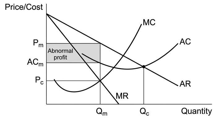
The diagram shows a monopoly earning abnormal profit at output Qm where MR = MC, charging price Pm. If contestability increases, barriers to entry fall. Potential entrants can enter quickly if they see abnormal profits, and exit without cost if conditions worsen. The threat of entry forces the incumbent to behave more competitively. To deter entry, the incumbent may lower price towards the competitive level where P = AC, earning only normal profit. Output rises to Qc and price falls to Pc. Consumers gain from lower prices and greater output. They may also benefit from increased choice and innovation as new firms enter. Producers lose their abnormal profits, but the pressure of competition may reduce X-inefficiency, lowering costs and improving productive efficiency. Some firms may become more dynamic to survive.
The case against – potential losses for consumers and producers
However, increased contestability may have negative effects. If the incumbent loses market share, it may be unable to exploit economies of scale, raising average costs. This could offset some of the price reduction for consumers. In industries with large sunk costs (e.g., natural monopolies), contestability is inherently limited. Forcing competition in such markets may lead to duplication of infrastructure and higher unit costs, harming both consumers (higher prices) and producers (lower profits). Moreover, the loss of abnormal profits may reduce funds available for research and development, undermining dynamic efficiency. Consumers may face less innovation in the long run.
Evaluation
The net impact depends on the degree of contestability achieved and the nature of the industry. In markets with low sunk costs (e.g., services, retail), increased contestability is likely to benefit consumers significantly through lower prices and better quality, while producers face pressure to become more efficient. In natural monopolies or industries with high sunk costs, contestability may be less effective and could even be welfare-reducing. The time horizon matters: short-run gains to consumers may come at the expense of long-run dynamic efficiency if firms cannot sustain investment.
Conclusion
On balance, an increase in market contestability generally benefits consumers through lower prices and greater choice, while producers lose abnormal profits but may gain efficiency. However, the outcome is not universally positive; in industries with significant economies of scale or high sunk costs, the benefits are limited and may be outweighed by losses in dynamic efficiency. Therefore, the impact depends critically on the specific market conditions.
An increase in market contestability generally benefits consumers through lower prices and greater output, while producers lose abnormal profits but may gain efficiency; however, in industries with high sunk costs or natural monopoly characteristics, the benefits are limited and dynamic efficiency may be harmed.
Background Concept
Market contestability is a concept developed by William Baumol. A perfectly contestable market is one where entry and exit are costless – there are no barriers to entry or exit, and no sunk costs. Sunk costs are costs that cannot be recovered upon exit (e.g., advertising, specialised equipment). In such a market, even a monopoly cannot earn abnormal profits in the long run because the threat of hit-and-run entry forces it to price at average cost (normal profit). The key insight is that the number of firms is less important than the ease of entry. Contestability theory challenges the traditional view that monopoly always leads to high prices and inefficiency.
Understanding the Question
The question asks you to evaluate the impact on consumers and producers of an increase in market contestability. You must use a diagram. The command word is 'evaluate', which requires a two-sided analysis and a justified conclusion. The mark scheme allocates 14 marks for AO1/AO2 (knowledge, understanding, analysis) and 6 marks for AO3 (evaluation). The top band for AO1/AO2 requires detailed knowledge, fully developed explanations, accurate use of diagrams fully explained, and a well-organised response. The top band for AO3 requires a justified conclusion with developed evaluative comments. The question is specific: impact on consumers AND producers, so both must be addressed.
Approach
Start by defining contestability and explaining the conditions. Then present a diagram of a non-contestable market (monopoly) showing abnormal profits. Explain how increased contestability (removal of barriers) changes the outcome: the threat of entry forces the incumbent to lower price and increase output, benefiting consumers. Then develop the counter-argument: potential loss of economies of scale, harm to dynamic efficiency, and the special case of natural monopolies. Evaluate by weighing the conditions under which each side dominates. Conclude with a justified judgement.
Step-by-Step Reasoning
-
Define contestability: A market is contestable if there are no barriers to entry or exit, especially no sunk costs. This allows potential entrants to enter quickly if they see profit and exit without loss.
-
Diagram: Draw a monopoly diagram. Label axes: Price/Cost and Quantity. Draw downward-sloping demand (AR) and MR. Draw U-shaped AC and MC. Show profit-maximising output Qm where MR=MC, price Pm from AR, and average cost at that output. Shade the abnormal profit rectangle (Pm - AC) x Qm. Explain that this is the situation before contestability increases.
-
Impact of increased contestability: When barriers fall, potential entrants can enter. The incumbent, to avoid losing market share, may lower price to the level where only normal profit is earned (P = AC). This is the contestable outcome. On the diagram, this would be at the point where AR = AC, typically at a higher output Qc and lower price Pc. Consumers gain consumer surplus (lower price, more output). Producers lose abnormal profit but may still earn normal profit. Additionally, the threat of entry may reduce X-inefficiency (the tendency of monopolies to have higher costs due to lack of competition), so AC may fall, further benefiting consumers.
-
Counter-arguments:
- If the incumbent loses market share, it may lose economies of scale, raising AC. This could offset some of the price reduction.
- In natural monopolies (e.g., water, electricity), average costs fall as output increases due to huge fixed costs. Splitting the market among several firms would raise costs. Contestability may not work because sunk costs are high (infrastructure). Forcing competition could lead to duplication and higher prices.
- Abnormal profits are often used for R&D. If they are eliminated, dynamic efficiency may suffer, leading to less innovation in the long run. Consumers may face higher prices or lower quality over time.
-
Evaluation: The net impact depends on:
- The degree of contestability: full contestability (no sunk costs) vs partial.
- The industry: low sunk costs (e.g., airlines, retail) vs high sunk costs (e.g., railways, pharmaceuticals).
- The time horizon: short-run gains vs long-run dynamic efficiency.
- The response of firms: some may become more efficient, others may exit.
-
Conclusion: On balance, consumers usually gain from lower prices and more choice, while producers lose abnormal profits but may become more efficient. However, in industries with significant economies of scale or high sunk costs, the benefits are limited and may be outweighed by losses in dynamic efficiency. Therefore, the impact is context-dependent, but the presumption is that increased contestability is beneficial in most markets.
Key Takeaways
- Contestability theory emphasises the role of potential competition, not just actual competition.
- A diagram is essential: show the monopoly equilibrium and the contestable outcome (normal profit).
- Evaluation must consider both sides: consumers vs producers, short run vs long run, different industry types.
- The conclusion must be justified, not just a summary.
Common Mistakes
- Omitting the diagram or drawing it without explanation (capped at L2).
- One-sided analysis: only discussing benefits to consumers without considering drawbacks.
- Confusing contestability with perfect competition: contestable markets can have few firms but still be efficient.
- Failing to define sunk costs and their role.
- Not addressing both consumers and producers explicitly.
- Providing a vague conclusion without weighing the arguments.
Things to Be Careful About
- Label all axes, curves, and equilibrium points on the diagram.
- Explain the diagram in the text – do not assume the diagram speaks for itself.
- Use economic terminology: abnormal profit, normal profit, sunk costs, barriers to entry, economies of scale, dynamic efficiency, X-inefficiency.
- Ensure the evaluation is developed: give reasons why one side may outweigh the other under specific conditions.
- The conclusion should directly answer the question: what is the impact on consumers and producers?
With the help of a diagram, assess the importance of the supply of labour in relation to the wage and employment levels for firms operating in perfectly competitive and monopsony labour markets.
Introduction
In a labour market, the wage and employment level are determined by the interaction of demand for labour (derived from marginal revenue product, MRP) and supply of labour. The structure of the labour market – whether perfectly competitive or monopsonistic – fundamentally affects how the supply of labour influences outcomes. This essay analyses the importance of labour supply in both market structures, using diagrams, and evaluates its relative significance.
Perfectly Competitive Labour Market
In a perfectly competitive labour market, there are many firms demanding labour and many workers supplying labour. Each firm is a wage-taker: it can hire any number of workers at the going market wage rate, Wc. The supply of labour to an individual firm is perfectly elastic (horizontal) at Wc. The firm’s demand for labour is its MRP curve, which slopes downward due to diminishing marginal returns. The profit-maximising firm hires labour up to the point where MRP = marginal cost of labour (MCL). Since MCL = Wc, the firm employs Lc workers where MRP = Wc.
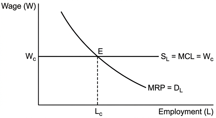
In this market, the supply of labour to the firm is perfectly elastic, so the wage is determined by market-wide forces (market demand and market supply). The firm’s employment level is determined by its own MRP. Thus, the supply of labour to the firm is important only in that it sets the wage; the firm cannot influence it. A change in market supply (e.g., an influx of workers) would lower the market wage and shift the firm’s supply curve down, leading to higher employment at the new wage.
Monopsony Labour Market
A monopsony exists when there is a single buyer of labour in a market. The firm faces an upward-sloping supply curve of labour (SL), because to attract more workers it must raise the wage for all workers. Consequently, the marginal cost of labour (MCL) lies above the supply curve. The monopsonist hires labour where MCL = MRP, at employment Lm, and pays the wage Wm given by the supply curve at that employment level. This results in a lower wage and lower employment than would occur in a competitive market (where the intersection of supply and demand would give Wc and Lc).
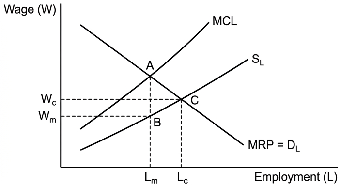
Here, the supply of labour is crucial: its upward slope directly causes the monopsonist to restrict employment and pay a lower wage. The elasticity of supply determines the gap between MCL and the wage; a steeper supply curve leads to a larger divergence and greater exploitation.
Evaluation
The importance of labour supply varies between the two market structures. In perfect competition, supply is important at the market level but not at the firm level (the firm is a price-taker). In monopsony, supply is central: the upward-sloping supply curve is the reason for lower wages and employment. However, other factors also matter:
- Demand-side factors: Changes in labour productivity (MRP) affect employment in both markets. In perfect competition, an increase in MRP raises employment but not the wage (since the firm still pays the market wage). In monopsony, an increase in MRP raises both employment and the wage (as the firm moves up the supply curve).
- Government intervention: A minimum wage set above Wm but below Wc can raise wages and employment in monopsony, effectively making the supply curve horizontal up to that wage. Trade unions can also bargain for higher wages, altering the effective supply.
- Market conditions: In perfect competition, a shortage of labour (supply shift left) raises the market wage and reduces employment in each firm. In monopsony, a supply shift left reduces employment further and raises wages.
Thus, while supply is always a determinant, its importance is magnified in monopsony because the firm exercises market power over the wage. In perfect competition, the wage is determined by market forces, and the firm’s employment decision is driven primarily by its MRP.
Conclusion
The supply of labour is more important in determining wage and employment levels in a monopsony labour market than in a perfectly competitive one, because the upward-sloping supply curve directly causes lower wages and employment. However, demand-side factors and institutional interventions can modify these outcomes, so the relative importance of supply must be assessed in context.
The supply of labour is more important in determining wages and employment in a monopsony labour market than in a perfectly competitive one, because the upward-sloping supply curve directly causes lower wages and employment; however, demand-side factors and institutional interventions can modify these outcomes.
Background Concept
Labour markets determine the wage rate and level of employment. The demand for labour is derived from the marginal revenue product (MRP) of labour – the additional revenue generated by hiring one more worker. MRP = marginal product × marginal revenue. In a perfectly competitive product market, MR = price, so MRP = marginal product × price. The demand curve for labour is the MRP curve, which slopes downward due to diminishing marginal returns.
The supply of labour to a firm depends on market structure. In a perfectly competitive labour market, there are many firms and many workers; each firm is a wage-taker and faces a perfectly elastic supply of labour at the market wage. In a monopsony, there is a single buyer of labour; the firm faces an upward-sloping supply curve because it must raise wages to attract more workers, and the marginal cost of labour (MCL) exceeds the wage.
Profit-maximising firms hire labour where MRP = MCL. In perfect competition, MCL = wage, so employment is where MRP = wage. In monopsony, MCL > wage, so employment is lower and wage is lower than in competition.
Understanding the Question
The question asks: "With the help of a diagram, assess the importance of the supply of labour in relation to the wage and employment levels for firms operating in perfectly competitive and monopsony labour markets." The command word "assess" requires evaluation – you must weigh the importance of supply relative to other factors and reach a justified conclusion. The question explicitly requires at least one diagram (the mark scheme caps at Level 2 without a diagram). You must discuss both market structures; the mark scheme says "Must refer to both markets for L3". The top band (AO1/AO2) demands detailed knowledge, fully developed explanations, accurate diagrams fully explained, and a well-organised response. The top AO3 band requires a justified conclusion with developed evaluative comments.
Approach
- Introduction: Define key terms (labour supply, MRP, perfect competition, monopsony) and state the essay's focus.
- Perfectly competitive labour market: Explain the characteristics, draw and explain the diagram showing the firm's perfectly elastic supply and MRP curve. Show how wage and employment are determined. Discuss the importance of supply: at the firm level, supply is perfectly elastic so the wage is given; at the market level, supply determines the wage.
- Monopsony labour market: Explain the characteristics, draw and explain the diagram showing upward-sloping supply, MCL above supply, and the monopsony equilibrium. Show how supply directly causes lower wage and employment.
- Evaluation: Compare the two markets. Consider factors that modify the importance of supply: changes in MRP, government intervention (minimum wage, unions), supply shocks. Weigh the relative importance.
- Conclusion: Provide a justified judgement answering the question.
Step-by-Step Reasoning
Perfect Competition
- Assume many firms, many workers, perfect information, homogeneous labour, no barriers to entry.
- Market demand for labour is the sum of firms' MRP curves; market supply is the sum of workers' willingness to work. The market wage Wc is determined by intersection of market demand and supply.
- Each firm takes Wc as given. Its supply of labour is perfectly elastic at Wc. The firm's demand for labour is its MRP curve (downward sloping).
- The firm hires Lc where MRP = Wc. At this point, the firm maximises profit.
- Diagram: Axes: Wage (W) and Employment (L). For the firm: horizontal supply curve at Wc, downward-sloping MRP curve. Equilibrium at (Lc, Wc).
- Importance of supply: The firm cannot influence the wage; supply is important only in that it sets the wage. If market supply increases (more workers), market wage falls, the firm's supply curve shifts down, and the firm hires more workers at the lower wage. So supply matters at the market level.
Monopsony
- Assume a single firm hiring labour in a market with many workers. The firm faces an upward-sloping supply curve SL (average cost of labour). To hire more workers, it must raise the wage for all workers, so the marginal cost of labour MCL lies above SL.
- The firm hires Lm where MCL = MRP. It then pays the wage Wm on the supply curve at that employment level.
- Diagram: Axes: Wage (W) and Employment (L). Upward-sloping SL, MCL above SL, downward-sloping MRP. Equilibrium: MCL = MRP at Lm, then go down to SL to find Wm. Also show the competitive equilibrium (where SL = MRP) at (Lc, Wc) for comparison.
- Importance of supply: The upward slope of supply is the reason for the monopsony outcome. If supply were perfectly elastic (as in competition), the firm would hire more and pay higher wage. The elasticity of supply determines the degree of exploitation: a steeper supply curve means a larger gap between MCL and wage, leading to lower wage and employment.
Evaluation
- In perfect competition, supply is important at the market level but not at the firm level. The firm's wage is determined by market forces, and its employment is driven by MRP. So supply is less important for the firm's decision.
- In monopsony, supply is central: the upward-sloping supply directly causes lower wage and employment. Without market power, the outcome would be different.
- However, other factors can alter the importance:
- Changes in MRP: In perfect competition, an increase in MRP (e.g., due to higher product price) shifts the firm's demand curve right, increasing employment but not the wage (since the firm still pays the market wage). In monopsony, an increase in MRP shifts the MRP curve right, increasing both employment and wage (as the firm moves up the supply curve). So demand-side changes can be more important in perfect competition for employment, while in monopsony both wage and employment respond.
- Government intervention: A minimum wage set above Wm but below Wc can make the supply curve horizontal up to that wage, turning the monopsonist into a wage-taker and raising employment. This reduces the importance of the upward-sloping supply. Similarly, trade unions can bargain for higher wages, effectively flattening the supply curve.
- Supply shocks: A decrease in labour supply (e.g., emigration) shifts the supply curve left. In perfect competition, this raises the market wage and reduces employment in each firm. In monopsony, it reduces employment further and raises wages. The effect is more pronounced in monopsony because the firm already restricts employment.
- Overall, the supply of labour is more important in monopsony because it is the source of market power and directly determines the wage-employment trade-off. In perfect competition, supply is important only at the market level, and the firm's behaviour is largely demand-driven.
Conclusion
The supply of labour is more important in a monopsony labour market than in a perfectly competitive one, because the upward-sloping supply curve is the mechanism through which the monopsonist restricts employment and pays lower wages. However, demand-side factors and institutional interventions can modify the outcomes, so the relative importance must be assessed in context. A justified conclusion would state that while supply is always a determinant, its significance is magnified in monopsony.
Key Takeaways
- In perfect competition, the firm faces a perfectly elastic supply of labour; wage is market-determined, employment is determined by MRP.
- In monopsony, the firm faces an upward-sloping supply; MCL > wage, leading to lower wage and employment than in competition.
- The supply of labour is more important in monopsony because it directly causes the inefficiency.
- Diagrams must be fully labelled and explained to earn top marks.
- Evaluation should consider demand-side changes, government intervention, and supply shocks.
Common Mistakes
- One-sided answer: Only discussing one market structure. The mark scheme requires both for Level 3.
- No diagram or unexplained diagram: The mark scheme caps at Level 2 without a diagram. Even with a diagram, if not explained, it may not reach top band.
- Confusing the firm's supply curve with market supply: In perfect competition, the firm's supply is perfectly elastic; the market supply is upward sloping. In monopsony, the firm faces the market supply curve.
- Not distinguishing between wage and MCL: In monopsony, the wage is not equal to MCL; this is a common error.
- Lack of evaluation: Simply describing both markets without weighing their importance or considering other factors will not score well on AO3.
- No conclusion or vague conclusion: The top AO3 band requires a justified conclusion.
Things to Be Careful About
- Label all axes (Wage, Employment) and curves (SL, DL/MRP, MCL, Wc, Lc, Wm, Lm).
- Show the competitive equilibrium on the monopsony diagram for comparison.
- Explain the diagrams in the text: what each curve represents, why they slope as they do, and what the equilibrium shows.
- Use correct terminology: "marginal revenue product", "marginal cost of labour", "perfectly elastic", "monopsony".
- In evaluation, avoid simply listing points; develop each point and link it to the question.
- The conclusion should directly answer the question about the "importance" of supply, not just summarise.
With the help of a diagram, evaluate the effectiveness of using monetary policy to increase the rate of economic growth in a country.
Introduction
Monetary policy involves the use of interest rates, the money supply, and exchange rate adjustments by a central bank to influence aggregate demand (AD). The rate of economic growth is measured as the increase in real GDP over time, which can be either actual (short-run) growth or potential (long-run) growth. This essay evaluates the effectiveness of expansionary monetary policy in stimulating actual and potential growth.
How monetary policy can increase growth
Expansionary monetary policy, such as reducing the policy interest rate, lowers the cost of borrowing. This encourages consumption and investment, shifting AD to the right. An increase in AD, assuming the economy is below full employment, leads to a rise in real GDP and thus actual growth.
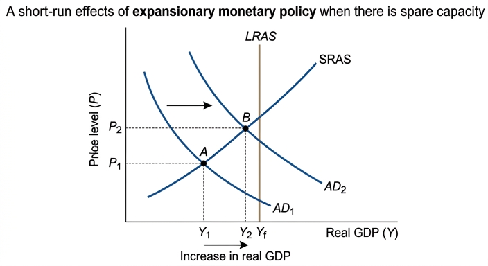
The diagram shows AD shifting from AD1 to AD2, moving the economy from point A to point B, with real GDP rising from Y1 to Y2. The short-run aggregate supply curve (SRAS) is upward-sloping, reflecting spare capacity. This illustrates how monetary policy can increase actual growth.
Similarly, quantitative easing (increasing the money supply) can reduce long-term interest rates and stimulate spending. Alternatively, a policy of devaluation (if the central bank manages the exchange rate) raises net exports, boosting AD, especially if the Marshall-Lerner condition holds.
Limitations and evaluation
The effectiveness of monetary policy depends on several factors:
- Spare capacity: If the economy is already at full capacity, expansionary policy will mainly cause inflation, not growth. The AD/AS diagram would show a vertical LRAS, so the increase in AD only raises the price level.
- Liquidity trap: When interest rates are already very low, further reductions may not stimulate borrowing and spending, as agents prefer to hold cash. Money supply increases may be hoarded rather than spent.
- Expectations and confidence: If consumers and firms are pessimistic (e.g., during a recession), lower interest rates may not induce significant consumption or investment. The impact on AD is muted.
- Inflation risk: Persistent expansionary policy may lead to higher inflation, which can harm long-term growth by reducing international competitiveness and creating uncertainty.
- Time lags: Monetary policy acts with a lag. The effect on growth may be delayed, reducing its effectiveness in responding to a downturn.
- Exchange rate effects: A devaluation can boost net exports, but its effectiveness depends on the Marshall-Lerner condition (sum of export and import demand elasticities > 1) and the J-curve effect (short-run worsening of trade balance before improvement).
- Supply-side constraints: If the economy's potential growth is low due to structural issues, monetary policy can only provide temporary growth. Long-term growth requires supply-side policies (investment in skills, infrastructure, innovation).
Evaluation
In the short run, monetary policy can be effective in increasing growth if the economy has spare capacity, low inflation expectations, and the transmission mechanism is working (e.g., banks are willing to lend, consumers are responsive). However, its effectiveness diminishes in a liquidity trap or when confidence is low. In the long run, monetary policy cannot raise the potential growth rate; it only addresses demand-side fluctuations. For sustained growth, it must be complemented by supply-side policies.
Conclusion
Monetary policy is a useful tool to increase economic growth in the short run, particularly during a recession with spare capacity. However, its effectiveness is limited by the liquidity trap, low confidence, and the risk of inflation. It is most effective when used alongside fiscal and supply-side policies, and when the economy is not at full capacity. Therefore, while it can contribute to growth, it is not a panacea and its effectiveness depends heavily on the prevailing economic conditions.
Monetary policy can increase economic growth in the short run when there is spare capacity and effective transmission, but it is limited by the liquidity trap, inflation risk, and inability to raise potential growth; it is most effective when complementing other policies.
Background Concept
Monetary policy refers to actions by a central bank to control the money supply and interest rates to achieve macroeconomic objectives. The main tools are the policy interest rate, reserve requirements, open market operations (quantitative easing), and exchange rate intervention. Economic growth is the increase in the productive capacity of the economy (potential growth) or the actual increase in real GDP (actual growth). The AD/AS model is the standard framework to analyse the impact of monetary policy on output and prices. Expansionary monetary policy shifts AD rightward, raising real GDP in the short run if the economy is operating below full employment (i.e., with a negative output gap).
Understanding the Question
The question asks you to evaluate the effectiveness of using monetary policy to increase the rate of economic growth. The command word 'evaluate' requires you to consider both the strengths and limitations of monetary policy in achieving this goal, and to reach a justified conclusion. The phrase 'with the help of a diagram' means you must draw and fully explain an AD/AS diagram. The question is worth 20 marks (14 for analysis, 6 for evaluation), so the answer must be a well-structured essay with developed analysis and a clear judgement. The top band requires detailed knowledge, fully developed explanations, accurate use of the diagram, and a justified conclusion.
Approach
Start by defining monetary policy and economic growth. Then explain the theoretical mechanism: how expansionary monetary policy (e.g., lower interest rates) increases AD, leading to higher real GDP. Use the AD/AS diagram to illustrate this. Then turn to the evaluation: discuss factors that limit effectiveness (liquidity trap, expectations, inflation, time lags, exchange rate conditions, supply-side constraints). Weigh the short-run vs long-run impact. Conclude with a judgement on when monetary policy is most effective and whether it is sufficient on its own.
Step-by-Step Reasoning
-
Define key terms: Monetary policy: central bank actions affecting interest rates, money supply, exchange rate. Economic growth: increase in real GDP (actual) or potential output. Effectiveness: the extent to which the policy achieves its intended goal without significant side effects.
-
Explain the theoretical case: A reduction in the policy rate lowers the cost of borrowing for consumers and firms. Consumption (C) and investment (I) increase, raising AD (C + I + G + X-M). In the AD/AS diagram, AD shifts right. If the economy is below full employment (spare capacity), the SRAS is relatively elastic, so the increase in AD leads to a rise in real GDP (from Y1 to Y2) with only a modest increase in the price level. This is actual growth. The diagram must be drawn and explained: label axes, AD1, AD2, SRAS, LRAS (if relevant), points A and B, and the change in Y.
-
Discuss quantitative easing: When interest rates are at the zero lower bound, central banks can increase the money supply by purchasing assets. This lowers long-term yields and encourages lending and spending. This can shift AD similarly.
-
Exchange rate channel: A lower interest rate may cause depreciation of the currency, making exports cheaper and imports dearer. Net exports (X-M) increase, boosting AD. This is effective if the Marshall-Lerner condition holds (sum of price elasticities of export and import demand > 1).
-
Introduce evaluation factors:
- Spare capacity: If the economy is at full employment (LRAS vertical), any increase in AD only causes inflation, not growth. The diagram would show price level rising but real GDP unchanged.
- Liquidity trap: When interest rates are near zero, agents may prefer to hold cash rather than spend or invest. Money supply increases are hoarded, so AD does not shift. This is a Keynesian critique.
- Expectations: If consumers expect deflation or are pessimistic, they may delay spending despite low interest rates. Similarly, firms may be reluctant to invest if demand is weak.
- Inflation: Persistent expansionary policy can lead to demand-pull inflation. High inflation reduces real income, hurts competitiveness, and may lead to higher interest rates in the future, dampening growth.
- Time lags: Monetary policy works with a lag (recognition, implementation, transmission). By the time the policy takes effect, the economic situation may have changed, potentially causing overheating.
- Exchange rate policies: Devaluation may not improve the trade balance if the Marshall-Lerner condition is not met, or due to the J-curve effect (short-run deterioration before improvement).
- Supply-side constraints: Monetary policy only affects demand. If low growth is due to low productivity, poor infrastructure, or labour market rigidities, monetary policy alone cannot raise potential growth. Supply-side policies are needed.
-
Weigh and conclude: In the short run, with spare capacity and normal transmission, monetary policy is effective. But its effectiveness is conditional. It is best used to stabilise the cycle, not to drive long-term growth. A justified conclusion: monetary policy is effective for short-run growth when there is a negative output gap, but it has limitations; for sustained growth, it must be part of a broader policy mix.
Key Takeaways
- The AD/AS model is essential for analysing the short-run impact of monetary policy on growth.
- Evaluation requires considering the economic context (spare capacity, expectations, interest rate environment).
- Monetary policy is a demand-side tool; it cannot increase potential growth on its own.
- A justified conclusion must weigh the conditions for effectiveness.
Common Mistakes
- Omitting the diagram or failing to explain it fully (labels, shift, equilibrium points).
- Presenting a one-sided argument: only discussing how monetary policy works without evaluating limitations.
- Confusing actual growth with potential growth.
- Ignoring the role of expectations and the liquidity trap.
- Providing a vague conclusion without a clear judgement.
- Not using economic terminology (e.g., 'spare capacity', 'transmission mechanism').
Things to Be Careful About
- Ensure the diagram is clearly labelled and the shift is in the correct direction.
- Distinguish between short-run and long-run effects.
- Use the extract's own data? Not applicable here, but in general, use given data.
- For the evaluation, structure it with clear points and link each to the effectiveness of monetary policy.
- The conclusion should directly answer the question: to what extent is monetary policy effective?
“The use of tariffs is the most effective way to correct a balance of payments deficit.”
With the help of a diagram, evaluate this statement.
Introduction
A balance of payments deficit on the current account occurs when a country's expenditure on imports of goods and services exceeds its revenue from exports. A tariff is a tax on selected imports, designed to raise their domestic price and switch expenditure from foreign to domestic goods. This essay evaluates whether tariffs are the most effective policy to correct such a deficit.
Analysis: how a tariff can correct a deficit
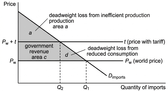
The diagram shows the domestic demand for imports (D_imports), which is downward sloping, and the world supply price (Pw), assumed to be perfectly elastic for a small country. Initially, the economy imports Q1 units at price Pw. The current account deficit includes Pw × Q1 of import expenditure.
A specific tariff of t per unit is imposed. The domestic price rises to Pw + t. Quantity of imports falls to Q2. The government collects tariff revenue of t × Q2 (area c). The value of imports at world prices falls from Pw × Q1 to Pw × Q2, so the current account improves by Pw × (Q1 − Q2). This is an expenditure-switching effect: domestic consumers switch to domestically produced substitutes.
The extent of the improvement depends on the price elasticity of demand for imports. If demand is price elastic, the quantity fall is large and the current account improves substantially. If demand is price inelastic, the quantity falls only a little; in that case total consumer expenditure on imports (including the tariff) actually rises, which may create inflationary pressure and offset some of the BOP improvement.
Evaluation
While the tariff can improve the current account in the short run, several limitations challenge the claim that it is the 'most effective' policy.
First, retaliation is highly likely. Trading partners may impose their own tariffs on the country's exports, reducing export revenue and potentially worsening the overall trade balance. The net effect may be zero or negative, especially if the country is part of a trading bloc or depends on export markets.
Second, the nature of the deficit matters. A temporary deficit caused by a cyclical boom may be better addressed by expenditure-reducing policies (fiscal or monetary tightening) that cool aggregate demand and reduce import spending without distorting trade. A persistent, structural deficit might require supply-side policies to improve competitiveness, such as investment in infrastructure or education, which address the root cause rather than merely suppressing imports.
Third, tariffs create deadweight welfare losses. They reduce consumer surplus (areas a + b + c + d in the diagram), of which area c is tariff revenue but areas a and d are deadweight losses – the loss from inefficient domestic production and the loss from reduced consumption. This reduces allocative efficiency and may harm long-run growth.
Fourth, alternatives exist. An exchange rate devaluation or depreciation can switch expenditure without creating tariff revenue or retaliation, provided the Marshall–Lerner condition holds. Expenditure-reducing policies (tighter monetary or fiscal policy) directly lower aggregate demand and import spending. Supply‑side policies improve productivity and export competitiveness over time. Each has its own drawbacks – devaluation may be inflationary; contractionary policy may raise unemployment – but none faces the same risk of tit‑for‑tat retaliation.
Conclusion
Tariffs can correct a balance of payments deficit in the short run by reducing import volumes, but they are not the most effective way overall. The risk of retaliation, the welfare losses they impose, and the availability of alternative policies that address underlying causes (such as supply-side reforms or exchange rate adjustment) mean that a single policy is unlikely to be 'most effective' in all circumstances. Their effectiveness is limited to situations where import demand is elastic and where retaliation is unlikely, and even then they are best used as part of a broader policy package rather than as a standalone solution.
Tariffs can improve the current account in the short run but are not generally the most effective policy due to the risk of retaliation, welfare losses, and the availability of alternative policies (expenditure-reducing, exchange rate, supply-side) that address the root causes of a deficit. Their effectiveness depends on the price elasticity of import demand, the nature and persistence of the deficit, and the likelihood of retaliation.
Background Concept
A balance of payments deficit on the current account occurs when the value of a country's imports of goods and services exceeds the value of its exports. This means the country is spending more foreign currency than it earns, which can put downward pressure on the exchange rate and require borrowing from abroad. A tariff is a tax imposed on imported goods. It raises the domestic price of those goods above the world price, making domestic products relatively cheaper. This is an example of an expenditure-switching policy – it aims to switch domestic spending away from imports and towards domestically produced substitutes, thereby improving the current account.
Tariffs belong to a broader class of protectionist trade policies. They differ from expenditure-reducing policies (such as contractionary fiscal or monetary policy) which reduce aggregate demand and therefore reduce spending on both imports and domestic goods. The effectiveness of a tariff depends critically on how strongly consumers respond to the price change – i.e. the price elasticity of demand for imports. It also depends on whether trading partners retaliate and on the underlying cause of the deficit (temporary versus structural).
Understanding the Question
The question asks you to evaluate the statement that "the use of tariffs is the most effective way to correct a balance of payments deficit." The word "most effective" makes this a comparative judgement: you must weigh tariffs against alternative policies (exchange rate adjustment, expenditure-reducing policies, supply-side policies) and decide whether tariffs are superior. The instruction "with the help of a diagram" means that a fully labelled and explained tariff diagram is required to reach the highest band. The diagram must show the market for imports, the effect of a tariff on price, quantity, and welfare.
A deficit can be caused by different factors: a cyclical boom (which creates a temporary deficit as imports rise with higher income), a structural lack of competitiveness (persistent deficit), or an overvalued exchange rate. The effectiveness of tariffs will vary with the cause. The statement's absolute language ("most effective") also invites you to challenge its claim – a one-sided answer that only argues in favour of tariffs cannot score evaluation marks. You must develop both the case for tariffs and the counter-arguments, then reach a justified conclusion.
Approach
- Define key terms (tariff, balance of payments deficit, current account) to establish knowledge.
- Present the tariff diagram and explain how a tariff can reduce import expenditure and improve the current account. This covers the analytical mechanism.
- Develop the first side – the case that tariffs work: they directly reduce import volumes, raise government revenue, and are quick to implement.
- Develop the second side – the limitations: retaliation, the need for elastic demand, welfare losses (deadweight loss), and the fact that tariffs do not address the root cause.
- Compare with alternative policies – devaluation/depreciation, expenditure-reducing policies, supply-side policies – explaining why each might be more or less effective than tariffs in different circumstances.
- Conclude with a justified judgement – tariffs can help in specific conditions (elastic demand, no retaliation, short-run) but are not the "most effective" across all scenarios.
The evaluation will rest on criteria such as time period (short-run vs long-run), elasticity (PED of imports), stakeholder effects (domestic consumers, producers, trading partners), and opportunity cost (welfare loss versus alternative use of policy instruments).
Step-by-Step Reasoning
Step 1 – Understanding the tariff diagram.
Start with the market for imports. The demand curve (D_imports) slopes downward, showing that as the domestic price of imports rises, the quantity demanded falls. The world supply is assumed to be perfectly elastic at price Pw (a small-country assumption – the country cannot influence the world price). Without a tariff, the domestic price equals Pw, and Q1 units are imported. The country's import expenditure is Pw × Q1.
Step 2 – Imposing the tariff.
Suppose the government imposes a specific tariff of t per unit. The domestic price rises to Pw + t. At this higher price, the quantity of imports demanded falls to Q2. The government collects tariff revenue equal to the rectangle t × Q2 (the area between Pw and Pw + t from quantity 0 to Q2). The value of imports at world prices becomes Pw × Q2, which is smaller than Pw × Q1. The current account therefore improves by the difference: Pw × (Q1 − Q2).
Step 3 – The role of elasticity.
The size of the improvement depends on how responsive import demand is to price. If demand is price elastic (PED > 1), the percentage fall in quantity is larger than the percentage rise in price, so the quantity falls substantially and the current account improves significantly. If demand is price inelastic (PED < 1), the quantity falls only a little, so the improvement in the current account is small. Moreover, total consumer expenditure on imports (including the tariff) = (Pw + t) × Q2. If demand is inelastic, this total actually rises, which means domestic consumers are spending more on imports than before (though part goes to the government as tax revenue). This can have inflationary effects and is one reason why tariffs may be ineffective.
Step 4 – Retaliation.
The analysis so far assumes no response from trading partners. In reality, other countries are likely to retaliate by placing their own tariffs on the country's exports. This reduces export revenue, which worsens the current account in the export sector. The net effect on the current account could be zero or negative. Retaliation is especially likely if the country is part of a trade agreement (e.g., WTO) or if it is a significant trading partner. This is one of the strongest arguments against tariffs as a general tool.
Step 5 – Nature of the deficit.
A deficit caused by a temporary cyclical boom may be self-correcting and best addressed by expenditure-reducing policies (e.g., tighter monetary policy) that cool demand without distorting trade patterns. A structural deficit (ongoing lack of competitiveness) may require supply-side policies to boost productivity and export quality. A deficit caused by an overvalued exchange rate may be best tackled by devaluation or depreciation. Tariffs treat the symptom (high imports) rather than the cause, and may create inefficiencies that persist after the deficit is corrected.
Step 6 – Welfare losses.
The tariff creates two deadweight losses: (i) the loss from inefficient domestic production – domestic producers expand output even though their costs exceed the world price, wasting resources (area a); (ii) the loss from reduced consumption – consumers who would have benefited from imports at the world price now pay more or go without (area d). These losses reduce allocative efficiency and harm long-run economic welfare, which is not directly captured in the current account figures but is an important broader cost.
Step 7 – Alternative policies compared.
- Exchange rate devaluation/depreciation: Switches expenditure without a tax, but may be inflationary and requires the Marshall–Lerner condition to hold. No tariff revenue, but no direct retaliation (though competitive devaluations can occur).
- Expenditure-reducing policies: Contractionary fiscal or monetary policy reduces aggregate demand, lowering imports. Effective for demand-pull deficits, but may cause unemployment and reduce growth. No market distortion from tariffs.
- Supply-side policies: Improve productivity, export quality, and long-run competitiveness. Slow to work but address the root cause; no trade war risk.
Step 8 – Reaching a judgement.
Weighing the arguments: tariffs have the advantage of being quick and directly targeting imports, and they raise revenue. However, the risk of retaliation, the need for elastic demand, the welfare losses, and the availability of alternative policies that address the cause mean tariffs are not the most effective policy overall. They may be suitable for a short-run, elastic-demand scenario with low risk of retaliation, but even then they should be part of a package. The word "most" in the statement overstates the case.
Key Takeaways
- Tariffs are an expenditure-switching policy: they raise the price of imports to reduce their quantity.
- The improvement in the current account depends on the price elasticity of demand for imports – elastic demand gives a larger improvement.
- Retaliation is a major limitation that can offset any gains.
- The cause of the deficit matters: tariffs treat symptoms, not underlying causes.
- Alternative policies (expenditure-reducing, exchange rate, supply-side) each have different strengths and weaknesses.
- A justified conclusion requires weighing both sides against explicit criteria (time period, elasticity, stakeholder impact).
- A diagram is compulsory for top marks – it must be fully labelled and explained in the text.
Common Mistakes
- One-sided argument: Only arguing that tariffs work (or don't). The command "evaluate" demands two sides; one side receives zero for AO3.
- No conclusion or a vague one: A summary of both sides without a judgement does not meet the top band. The conclusion must state which side is stronger and why.
- Omitted or poorly explained diagram: The mark scheme caps at L3 without a diagram. The diagram must be fully labelled (axes, curves, price levels, quantities, and welfare areas) and the explanation must walk through the shift.
- Ignoring retaliation: Many students analyse tariffs in isolation from the international response. This loses evaluation marks.
- Confusing expenditure-switching with expenditure-reducing: Tariffs switch expenditure; monetary/fiscal tightening reduces total expenditure. Mixing them up shows poor understanding.
- Assuming all deficits are the same: The effectiveness of tariffs depends on whether the deficit is cyclical, structural, or exchange-rate-driven.
- Using a micro diagram (e.g., domestic supply and demand for a single good) without explanation: While the diagram is micro, it must be explicitly linked to the current account and import expenditure.
Things to Be Careful About
- Diagram labels: Label the axes (Price and Quantity of imports), the curves (D_imports, world supply at Pw, world supply + tariff at Pw+t), and the equilibrium quantities (Q1, Q2). Show the tariff revenue rectangle and the deadweight loss triangles if possible.
- Elasticity usage: State clearly that it is the price elasticity of demand for imports that matters, not the elasticity of domestic demand for the product in general.
- Short run vs long run: Tariffs may work in the short run but lead to retaliation or inefficient domestic industries in the long run. Distinguish the time frame in your evaluation.
- Real-world examples: While not required, mentioning a specific case (e.g., US–China trade war) can strengthen evaluation by illustrating retaliation.
- Avoid fence-sitting: The conclusion should not be "it depends" without saying what it depends on and which way the scales tip under typical circumstances. Give a conditional but decisive judgement.
- Formatting: Use clear headings and logical flow. The top band rewards "well-organised, well-focused and presented in a logical and coherent manner."