Economics 9708/42 — October/November 2025
Cambridge A-Level · A Level Data Response and Essays · worked solutions for every part, with the mark scheme
Topics Externalities, Social Costs and Benefits · Economic Development and Living Standards · Growth and Survival of Firms · Market Structures · Government Policies to Correct Market Failure · Demand for and Supply of Labour · +4 more
Resources in Brazil
Between 2000 and 2020, Brazilian GDP, measured in US dollars ($), rose from $1.19 trillion to $1.89 trillion at constant prices (2015). In the same period GDP per head rose from $6745 to $8204 at constant prices (2015).
The strength of the Brazilian economy lies in the variety and quantity of its natural resources. For example, Brazil is one of the world’s largest exporters of agricultural commodities, mainly soya and beef. There are also significant exports of minerals. Brazil is the second largest iron ore producer in the world and extracts 3.4% of the world’s crude oil.
World agricultural markets are dominated by four large commodity traders that buy and sell products such as grain and soya. They have grown through both horizontal integration and vertical integration. These traders own many large farms, they process farm produce and transport it to trade on international markets. In addition to buying and selling, the traders provide seed and fertiliser to farmers and supply storage for their products. They use agricultural by-products to produce items like biofuel. These traders also provide financial services to these markets.
Commodity traders are very important to the development of complex global food markets. Food prices, access to scarce resources such as land and water, climate change and food security are all affected by the activities of traders. In Brazil, the output of 15 000 farmers is purchased by a single trader.
In Brazil the development of agriculture, mining and oil extraction all contribute to environmental degradation. Both agriculture and mining have been accompanied by deforestation of the Amazon rainforest. Access roads to mining areas also lead to deforestation. Waste water from mining activity is frequently stored in reservoirs behind dams. On two occasions in the last 10 years these dams failed to hold back the water. This led to widespread flooding, the discharge of pollutants such as mercury into rivers, and deaths.
Sources: The Guardian, 23 August 2022
Cereal Secrets, Oxfam Research Report, August 2012
oec.world/en/profile, August 2023
Answer
GDP measures the total value of goods and services produced within a country. When GDP is measured at constant prices, the effects of inflation are removed by using the prices of a base year. This ensures that changes in GDP reflect only changes in the volume of output, not changes in prices. The significance is that it allows for meaningful comparisons of real output over time, showing whether an economy has grown in real terms.
Constant prices allow comparison of real output over time by removing the effect of price changes.
Background Concept
Gross Domestic Product (GDP) is the total market value of all final goods and services produced within a country's borders in a given period. Nominal GDP is measured at current prices and can increase either because output rises or because prices rise. To isolate changes in output, economists use constant prices (also called real GDP) by fixing the price level of a base year. This is done using a price index (e.g., GDP deflator) to adjust nominal GDP.
Understanding the Question
The question asks for the significance of measuring GDP at constant prices. It is a 3-mark point-based question. The mark scheme awards 1 mark for defining GDP, 1 mark for explaining that constant prices remove price changes, and 1 mark for stating that this allows measurement of real change. The candidate should provide a clear explanation of why this adjustment matters.
Approach
Start by defining GDP briefly. Then explain what constant prices mean and how they adjust for inflation. Finally, state the significance: real GDP comparisons over time. No diagram is needed.
Step-by-Step Reasoning
- Define GDP: total output of a country. This establishes the context.
- Explain constant prices: using base year prices to value output, so that price changes are eliminated.
- Significance: allows comparison of real output across years, showing true economic growth. Without this, an increase in nominal GDP could be due to inflation, misleading assessment of economic performance.
Key Takeaways
- Real GDP adjusts for inflation, reflecting actual changes in production.
- Constant prices enable meaningful time-series comparisons.
- This is a fundamental concept for understanding macroeconomic growth.
Common Mistakes
- Confusing nominal and real GDP.
- Stating only that constant prices remove inflation without explaining why that is important.
- Omitting the definition of GDP, which may lose a mark.
Things to Be Careful About
- Ensure the answer clearly links constant prices to the ability to measure real change.
- Use precise language: 'constant prices', 'real output', 'base year'.
- Do not include extraneous information about GDP per capita or other measures.
Explain one possible benefit of horizontal integration and one possible benefit of vertical integration.
Answer
Horizontal integration is the merger of firms at the same stage of production. A benefit is that it can lead to economies of scale, reducing average costs and increasing market share. Vertical integration is the merger of firms at different stages of production. A benefit of backward vertical integration is that it secures the supply of inputs, reducing uncertainty and transaction costs, which can improve efficiency and profitability.
Horizontal integration can achieve economies of scale; vertical integration can secure supply chains and reduce costs.
Background Concept
Integration refers to the combination of firms to increase size and control. Horizontal integration occurs between firms in the same industry and same stage of production (e.g., two grain traders merging). Vertical integration occurs between firms at different stages of production (e.g., a trader buying a farm for backward integration, or a processor buying a retailer for forward integration). The extract mentions that commodity traders have grown through both horizontal and vertical integration, owning farms, processing, transport, etc.
Understanding the Question
This is a 4-mark point-based question: 2 marks for horizontal integration (definition + benefit) and 2 marks for vertical integration. The command word is 'Explain', so a brief description of the benefit is required. The extract provides context but the answer can be general.
Approach
Define each type of integration, then give one clear benefit. For horizontal integration, focus on economies of scale or market power. For vertical integration, focus on supply security or cost reduction. Use the extract's example of traders owning farms to illustrate backward integration.
Step-by-Step Reasoning
- Horizontal integration: definition - merger of firms at same stage. Benefit: economies of scale (e.g., bulk purchasing, shared overheads) or increased market share leading to market power.
- Vertical integration: definition - merger of firms at different stages. Backward integration benefit: securing inputs, reducing transaction costs. Forward integration benefit: control over distribution. Choose one clear benefit.
- No need to compare both; just state each separately.
Key Takeaways
- Horizontal integration reduces competition and can lower costs.
- Vertical integration improves supply chain control and efficiency.
- Both are common strategies for firm growth.
Common Mistakes
- Confusing horizontal and vertical integration.
- Giving a benefit that is not specific to the type (e.g., saying 'increases profits' for both).
- Omitting the definition, which loses a mark.
Things to Be Careful About
- Ensure the benefit is clearly linked to the integration type.
- Use the extract to show application if relevant, but not required.
- Keep each part concise to fit the mark allocation.
Describe how the market structure in which individual farmers operate is likely to differ from the market structure in which the commodity traders operate.
Answer
Farmers are likely to operate in a market structure of monopolistic competition. There are many farmers (15 000 supply one trader), they produce a similar product (soya, beef), barriers to entry are low, and each farmer has some degree of market power due to slight product differentiation, making them price makers. In contrast, commodity traders operate in an oligopoly. The extract states that four large traders dominate world agricultural markets. This small number of firms means high barriers to entry (e.g., capital, control over processing and transport), product differentiation, interdependence, and price-making ability. The key difference is the number of firms and the degree of market power.
Farmers: monopolistic competition (many sellers, low barriers, price makers); Traders: oligopoly (few sellers, high barriers, interdependence).
Background Concept
Market structures describe the competitive environment of a market. Key characteristics include number of firms, product differentiation, barriers to entry, and the degree of market power. Monopolistic competition has many firms, differentiated products, low barriers, and some price-making power. Oligopoly has few firms, high barriers, interdependence, and significant market power. The extract provides clues: 15 000 farmers vs 4 large traders.
Understanding the Question
This is a 6-mark point-based question, split 3 marks for farmers and 3 marks for traders. The command word 'Describe' requires a clear explanation of the market structure for each group, including characteristics. The answer must correctly identify the market structure to earn marks for explanation.
Approach
First, identify the market structure for farmers: monopolistic competition (or possibly perfect competition, but the mark scheme specifies monopolistic competition). Then describe the characteristics: many sellers, similar product, low barriers, price maker. Then identify the structure for traders: oligopoly. Describe: few sellers, high barriers, product differentiation, interdependence, price maker. Contrast the two.
Step-by-Step Reasoning
- Farmers: Number of sellers - many (15 000 supplying one trader). Product - soya, beef, likely similar but not identical (location, quality differences). Entry - low barriers (farming relatively easy to enter). Market power - each farmer has some pricing power due to differentiation, but limited. Hence monopolistic competition.
- Traders: Number of sellers - few (four large traders dominate). Product - may be differentiated by brand, service, scope. Entry - high barriers (need large capital, control over supply chain, financial services). Market power - significant, each trader can influence price. Interdependence - actions of one affect others. Hence oligopoly.
- Contrast: farmers face many competitors, traders face few; farmers have low barriers, traders have high barriers; farmers are price takers? No, they are price makers in monopolistic competition, but much less power than traders. The key difference is degree of market power.
Key Takeaways
- Market structure is determined by number of firms, product differentiation, and barriers to entry.
- Monopolistic competition and oligopoly differ greatly in firm size and market power.
- Extract evidence is crucial for supporting the description.
Common Mistakes
- Identifying the wrong market structure (e.g., perfect competition for farmers).
- Describing characteristics without linking to the extract.
- Forgetting to mention the number of firms for both.
Things to Be Careful About
- The mark scheme explicitly requires the correct market structure for each to earn explanation marks.
- Use the extract's numbers: 15 000 farmers and 4 traders.
- Do not confuse the two structures; keep the description separate.
Use the article to evaluate the impact of the development of the agricultural and mining industries on the standard of living in Brazil.
Answer
Standard of living encompasses both monetary and non-monetary aspects. Monetary indicators include GDP per capita, while non-monetary indicators cover health, education, environment, and other quality-of-life factors.
Positive impacts on Brazil's standard of living from the development of agriculture and mining include a significant increase in real GDP from $1.19 trillion to $1.89 trillion (2015 constant prices) and a rise in GDP per capita from $6,745 to $8,204. This suggests higher average incomes, which can improve material living standards. Additionally, Brazil's large exports of agricultural and mineral commodities generate foreign exchange and employment, further boosting income.
However, there are substantial negative impacts on non-monetary aspects of living standards. The extract states that the development has led to deforestation of the Amazon rainforest, environmental degradation, and pollution from mining waste water, which caused flooding and mercury discharge. These environmental damages reduce quality of life, harm health, and threaten sustainability. The extract does not provide data on improvements in health, education, or housing, which are important non-monetary dimensions.
Overall, while the data shows clear monetary gains, the environmental costs and lack of information on other non-monetary indicators suggest that the impact on overall standard of living is mixed. A full assessment would require a broader set of indicators including health, education, and environmental quality. Therefore, it is not possible to conclude that development has unambiguously improved the standard of living, as the negative externalities may offset the monetary gains.
Monetary indicators show improvement but environmental degradation reduces non-monetary quality of life; the impact is mixed and requires further data.
Background Concept
Standard of living is a broad concept that includes both material well-being (income, consumption) and non-material aspects (health, education, environment, leisure, political freedom). Monetary indicators like GDP per capita are commonly used but incomplete. Non-monetary indicators such as life expectancy, literacy rates, pollution levels, and access to services provide a more comprehensive picture. Externalities, particularly negative externalities of production (e.g., pollution), reduce social welfare and thus lower standard of living, even if GDP rises.
Understanding the Question
This is a 7-mark point-based evaluative question. The command word 'evaluate' requires a two-sided discussion and a conclusion. The mark scheme allocates: up to 2 marks for defining standard of living (monetary and non-monetary), up to 4 marks for using extract data to discuss both positive and negative impacts, and 1 mark for a conclusion. The extract provides specific data on GDP and GDP per capita increases, as well as environmental degradation. The answer must use this evidence.
Approach
- Define standard of living, covering both monetary and non-monetary aspects.
- Present the positive impacts using extract data: GDP growth, GDP per capita increase, export strength.
- Present the negative impacts using extract data: deforestation, pollution, dam failures.
- Note that the extract lacks data on other non-monetary indicators like health and education.
- Conclude that while monetary indicators improved, environmental costs are significant, and without further data a definitive judgement is not possible. The conclusion should be balanced and justified.
Step-by-Step Reasoning
- Definition: Standard of living includes monetary (GDP per capita) and non-monetary (environment, health, education) aspects. This is worth up to 2 marks.
- Positive: From the extract, real GDP rose from $1.19 trillion to $1.89 trillion, GDP per capita from $6,745 to $8,204. This indicates higher average income, improving material living standards. Brazil is a large exporter of agricultural and mineral products, generating income and employment. (Up to 2 marks for data interpretation.)
- Negative: The extract mentions deforestation of the Amazon, pollution from mining waste water, and dam failures causing flooding and mercury pollution. These are negative externalities that harm health and the environment, reducing non-monetary living standards. (Up to 2 marks for data interpretation.)
- Additional limitation: The extract does not provide data on education, health, or housing, which are important non-monetary aspects. This is a weakness in the evidence. (The mark scheme mentions this.)
- Conclusion: The impact is mixed. Monetary gains are clear, but environmental degradation is significant. Without a broader set of indicators, a full evaluation cannot be made. The conclusion should be balanced and justified, not a simple summary. (1 mark for conclusion.)
Key Takeaways
- Standard of living is multidimensional; monetary indicators alone are insufficient.
- Development can have both positive income effects and negative environmental externalities.
- Evaluation requires weighing different aspects and acknowledging data limitations.
- A good conclusion is justified and specific to the question.
Common Mistakes
- Only discussing monetary impacts (one-sided) – loses evaluation marks.
- Not using extract data (e.g., quoting GDP figures) – loses data interpretation marks.
- Omitting the definition of standard of living – loses up to 2 marks.
- Providing a conclusion that is a vague summary rather than a justified judgement.
- Failing to mention the lack of non-monetary data as a limitation.
Things to Be Careful About
- Use the exact figures from the extract: $1.19 trillion, $1.89 trillion, $6,745, $8,204.
- Clearly separate positive and negative impacts.
- The conclusion should explicitly state that the overall impact is mixed and that a full assessment requires more data – this is the justified judgement.
- Do not introduce new concepts not in the extract; stick to what is given.
Traffic congestion is a cause of allocative inefficiency.
Evaluate, with the help of diagram(s) two policies that a government may introduce to reduce the problem of allocative inefficiency caused by traffic congestion.
Introduction
Traffic congestion arises because individual drivers ignore the external costs they impose on others, leading to a negative consumption externality. This results in allocative inefficiency, where the marginal social benefit (MSB) of road use is less than the marginal private benefit (MPB), causing overconsumption. The government can implement policies to internalise this externality and move the market towards the socially optimal level of road use. This essay evaluates two such policies: a congestion charge (an indirect tax) and a subsidy for public transport.
Policy 1: Congestion Charge
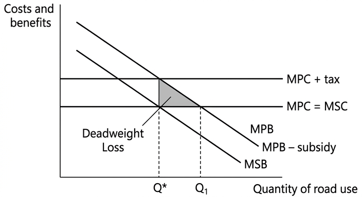
A congestion charge is a tax levied on drivers entering a congested area during peak times. It increases the private cost of driving, shifting the marginal private cost (MPC) curve upward to MPC+tax. As shown in the diagram, the initial market equilibrium is at Q1 where MPB = MPC, but the social optimum is at Q* where MSB = MSC. The congestion charge raises the cost to drivers, reducing the quantity of road use to Q*, thereby eliminating the deadweight welfare loss (the shaded area). This policy directly addresses the externality by making drivers pay the full social cost of their journey.
Evaluation of Congestion Charge
- Effectiveness: The charge is effective if it is set at the correct level to equate MPC+tax with MSC. However, estimating the exact external cost is difficult, and the charge may need to be adjusted over time.
- Equity: The charge may be regressive, disproportionately affecting lower-income drivers. However, revenue can be used to improve public transport or provide rebates.
- Behavioural response: The effectiveness depends on the price elasticity of demand for road use. If demand is inelastic, the charge may reduce congestion only slightly but generate significant revenue.
- Political feasibility: Congestion charges often face public opposition and may be costly to implement and enforce.
Policy 2: Subsidy for Public Transport
A subsidy for public transport reduces the cost of alternatives to driving, such as buses and trains. This lowers the opportunity cost of using public transport, effectively reducing the private benefit of driving. In the diagram, this can be represented as a downward shift of the MPB curve to MPB-subsidy, as drivers now derive less relative benefit from driving. The new equilibrium occurs at Q*, again eliminating the deadweight loss. The subsidy encourages a modal shift from private cars to public transport, reducing congestion.
Evaluation of Subsidy for Public Transport
- Effectiveness: The subsidy is effective if public transport is a close substitute for driving. If public transport is inconvenient or unreliable, the subsidy may have little impact on congestion.
- Cost: Subsidies require government expenditure, which has an opportunity cost. The funds could be used for other priorities such as healthcare or education.
- Demand elasticity: The price elasticity of demand for public transport determines the extent of modal shift. If demand is inelastic, a large subsidy may be needed to achieve a significant reduction in congestion.
- Indirect effects: Improved public transport can have positive externalities, such as reduced pollution and improved accessibility.
Overall Evaluation
Both policies can reduce allocative inefficiency, but they operate through different mechanisms. The congestion charge directly internalises the externality by raising the private cost to the social cost, making it a more targeted and potentially more efficient policy. However, it may be regressive and politically unpopular. The subsidy for public transport is more politically acceptable and can have wider benefits, but its effectiveness depends on the quality and convenience of public transport. A combination of both policies, using revenue from the congestion charge to fund public transport subsidies, may be the most effective approach.
Conclusion
In conclusion, both a congestion charge and a subsidy for public transport can help correct the allocative inefficiency caused by traffic congestion. The congestion charge is more direct in internalising the externality, while the subsidy addresses the problem indirectly. The optimal policy mix depends on the specific context, including price elasticities, equity considerations, and political feasibility. A well-designed congestion charge combined with improved public transport is likely to be the most effective solution.
A congestion charge is more direct and targeted, but a combination with a subsidy for public transport is likely to be the most effective solution.
Background Concept
Allocative efficiency occurs when resources are allocated to maximise consumer satisfaction, achieved when the marginal social benefit (MSB) equals the marginal social cost (MSC) for the last unit produced or consumed. Traffic congestion is a classic example of a negative consumption externality: each additional driver imposes a cost on others (time lost, increased pollution) that is not reflected in the private cost of driving. This leads to a divergence between the marginal private benefit (MPB) and the marginal social benefit (MSB), with MPB > MSB. The market equilibrium (where MPB = MPC) results in overconsumption (Q1 > Q*), creating a deadweight welfare loss. Government intervention aims to internalise this externality and move the market to the socially optimal output Q*.
Understanding the Question
The question asks you to evaluate two government policies to reduce allocative inefficiency caused by traffic congestion, using diagram(s). The command word 'evaluate' requires you to present both the strengths and weaknesses of each policy and reach a justified conclusion. The top band for AO1/AO2 demands detailed knowledge, fully developed explanations, and accurate use of diagrams that are fully explained. The top band for AO3 requires a justified conclusion with developed evaluative comments. You must address the specific problem of allocative inefficiency, not just congestion in general.
Approach
- Define allocative efficiency and explain how traffic congestion causes a negative consumption externality, leading to overconsumption and a deadweight loss.
- Draw a diagram showing the market for road use with MPB, MSB, MPC, MSC, the market equilibrium Q1, the social optimum Q*, and the deadweight loss.
- Analyse the first policy: a congestion charge (indirect tax). Explain how it shifts the MPC curve upward, reducing quantity to Q*. Evaluate its effectiveness, equity, behavioural response, and political feasibility.
- Analyse the second policy: a subsidy for public transport. Explain how it shifts the MPB curve downward (or increases the opportunity cost of driving), also leading to Q*. Evaluate its effectiveness, cost, demand elasticity, and indirect effects.
- Provide an overall evaluation comparing the two policies, considering their relative merits and drawbacks.
- Conclude with a justified judgement that addresses the specific question, possibly recommending a combination of policies.
Step-by-Step Reasoning
Step 1: The Externality Diagram
Draw a diagram with 'Quantity of road use' on the horizontal axis and 'Costs and benefits' on the vertical axis. The MPB curve slopes downward, representing the diminishing private benefit of additional driving. The MSB curve lies below MPB, reflecting the external congestion cost (the difference is the marginal external cost). Assume constant marginal private cost (MPC) and marginal social cost (MSC) are equal and horizontal (no production externality). The market equilibrium is at Q1 where MPB = MPC. The social optimum is at Q* where MSB = MSC. The deadweight loss is the triangle between Q* and Q1, bounded by MPB and MSB.
Step 2: Congestion Charge
A congestion charge is a specific tax per journey. It increases the private cost of driving, shifting the MPC curve upward by the amount of the tax to MPC+tax. The new equilibrium is where MPC+tax = MPB, which occurs at Q*. The tax internalises the externality by making drivers pay the full social cost. The revenue generated can be used to compensate losers or fund alternatives.
Evaluation: The charge is effective if set correctly, but estimating the external cost is difficult. It may be regressive, but revenue recycling can mitigate this. If demand for road use is inelastic, the charge may not reduce congestion much but raises revenue. Political opposition is common.
Step 3: Subsidy for Public Transport
A subsidy reduces the price of public transport, making it a more attractive alternative. This reduces the private benefit of driving relative to public transport, effectively shifting the MPB curve downward to MPB-subsidy. The new equilibrium is where MPB-subsidy = MPC, again at Q*. The subsidy encourages modal shift.
Evaluation: The subsidy is effective if public transport is a close substitute. If public transport is poor, the subsidy may have little effect. It requires government spending with opportunity cost. The price elasticity of demand for public transport determines the extent of shift. Positive externalities from reduced pollution and improved accessibility are additional benefits.
Step 4: Overall Evaluation
Compare the two policies: the congestion charge directly targets the externality and is more efficient in theory, but faces equity and political issues. The subsidy is more politically palatable but less direct and may be costly. A combination can be synergistic: use congestion charge revenue to fund public transport subsidies, addressing both efficiency and equity.
Step 5: Conclusion
A justified conclusion should state which policy or combination is likely to be most effective, given the context. For example: 'A congestion charge is more direct and efficient, but its regressive nature can be offset by using revenue to subsidise public transport, making a combined approach the most effective solution.'
Key Takeaways
- Negative consumption externalities cause allocative inefficiency by leading to overconsumption.
- Diagrams are essential to illustrate the divergence between private and social costs/benefits and the deadweight loss.
- Indirect taxes (congestion charges) internalise externalities by raising private costs to social costs.
- Subsidies for alternatives reduce the private benefit of the externality-generating activity.
- Evaluation must consider effectiveness, equity, elasticity, political feasibility, and opportunity cost.
- A justified conclusion is required for top marks.
Common Mistakes
- One-sided evaluation: only discussing advantages or disadvantages of each policy, not both.
- Not using a diagram or not explaining it fully (e.g., leaving axes unlabelled).
- Confusing a negative consumption externality with a production externality.
- Failing to link the policies explicitly to allocative efficiency (i.e., not showing how they move the market to Q*).
- Providing a vague conclusion that does not address the specific question.
- Listing many policies without developing any in depth.
Things to Be Careful About
- Label all axes and curves clearly on the diagram.
- Explain the diagram in the text, not just present it.
- Distinguish between private and social curves and show the direction of shifts.
- Consider the price elasticity of demand for road use and public transport when evaluating effectiveness.
- Address equity implications and how they might be mitigated.
- Ensure the conclusion is justified and specific, not a general summary.
The average wage of chief executives in large companies in a country is over 100 times greater than the average wage of their employees.
Assess how economic theory can account for this variation in average wages.
Introduction
The vast difference between the average wage of chief executives (CEs) and that of their employees can be analysed using labour market theory. In a perfectly competitive labour market, wages are determined by the interaction of demand and supply, where the demand for labour is derived from its marginal revenue product (MRP). This essay will explain how differences in MRP and labour supply conditions can account for wage variation, and then evaluate the limitations of this framework.
Analysis: Labour Demand and Supply
The demand for labour is a derived demand; firms hire workers as long as the extra revenue from employing one more unit (MRP) exceeds the marginal cost of that labour (the wage). MRP = marginal physical product (MPP) x price of output. Chief executives typically have a very high MPP – their decisions affect the entire company’s output and profitability. For example, a CE who successfully expands markets or improves efficiency can raise the firm’s value by millions, so their MRP is extremely high. In contrast, a typical employee’s MPP is limited to a specific task, and its impact on company revenue is much smaller.
On the supply side, the market for CEs is small and highly specialised. The supply of individuals with the necessary skills, experience and leadership ability is very inelastic. Acquiring these skills requires extensive education, training and a long track record, which acts as a barrier to entry. This inelastic supply means that even a modest increase in demand for CEs will drive up their wages substantially. Conversely, the supply of ordinary workers is often more elastic because there are many potential employees with the required qualifications, and entry barriers are lower.
Combining demand and supply, the equilibrium wage for CEs is high because demand (MRP) is high and supply is inelastic. For typical workers, lower MRP combined with more elastic supply results in a much lower equilibrium wage.
Economic Rent and Transfer Earnings
The concept of economic rent further explains the differential. The wage of a CE contains a large element of economic rent – the payment above the minimum necessary to keep them in their current job (transfer earnings). Since the supply of CEs is highly inelastic, most of their wage is economic rent. For ordinary workers, supply is more elastic, so a larger proportion of their wage is transfer earnings, and the rent element is smaller. This difference reinforces the overall wage gap.
Evaluation
While marginal productivity theory provides a coherent framework, its application to CE pay faces several problems. First, measuring the MRP of a CE is extremely difficult because their contribution is indirect and depends on many factors outside their control. Second, CE pay is often set by remuneration committees composed of other CEs, which can lead to upward bias (‘rent-seeking’). This suggests that CE wages may exceed their true MRP.
Third, the labour market for ordinary workers is not perfectly competitive. Many firms have monopsony power – they are the dominant employer in a local area and can pay workers less than their MRP. This widens the gap. Additionally, discrimination and prejudice can lower the wages of certain groups, making the observed variation partly a result of market failures rather than pure productivity differences.
Conclusion
Economic theory offers a powerful explanation for the variation in average wages: differences in MRP and labour supply conditions can account for a large part of the CEO–worker pay gap. However, the extreme magnitude of the gap – over 100 times – is unlikely to be explained solely by competitive market forces. Market imperfections such as monopsony power, rent-setting in CEO compensation, and discrimination also play significant roles. Therefore, while the standard demand-and-supply framework is a necessary starting point, it must be supplemented with institutional and behavioural factors to fully account for the observed variation.
Economic theory explains wage differentials primarily through differences in marginal revenue product and supply conditions; however, the extreme CEO-worker pay gap also reflects market failures such as monopsony power in labour markets, imperfect information, and rent-seeking, making the theory a partial but incomplete account.
Background Concept
This question requires an understanding of how wages are determined in labour markets. The core theory is the marginal productivity theory of wages, which states that in a perfectly competitive labour market, the wage rate is determined by the intersection of labour demand (the value of the marginal product of labour, MRP) and labour supply. The MRP is the additional revenue generated by employing one more unit of labour, calculated as MRP = MPP x P (marginal physical product multiplied by the price of output).
Under perfect competition, workers are paid the value of their marginal contribution because firms maximise profit by hiring labour up to the point where MRP = wage. However, real-world labour markets often deviate from perfect competition due to monopsony power, trade unions, discrimination, and imperfect information. The concepts of economic rent and transfer earnings help analyse wages: economic rent is the portion of a worker's wage that exceeds the minimum required to keep them in their job; transfer earnings are the minimum payment needed to keep them from moving to another job.
Understanding the Question
The question asks you to "assess how economic theory can account for this variation in average wages." The key fact is that chief executives earn over 100 times the average wage of employees. You need to explain why this huge gap exists using economic theory, and then evaluate how well the theory explains it. The command word "assess" requires a two-sided discussion: first, present the theoretical explanation (how demand and supply, MRP, and economic rent account for the gap), and second, identify limitations and alternative explanations (e.g., difficulties measuring MRP, monopsony, rent-seeking, discrimination). A final judgement is required.
This is a levels-marked essay (20 marks, AO1+AO2 out of 14, AO3 out of 6). To achieve the top band (11–14 for analysis), you must provide detailed, well-developed explanations supported by examples where appropriate. For evaluation (4–6), you must offer a justified conclusion with developed, reasoned evaluative comments.
Approach
- Start with an introduction that defines the theoretical framework and states what you will do.
- First, explain the basic theory: wages are determined by MRP and labour supply. Apply it to both CEs and workers: CEs have high MRP (because their decisions affect whole company) and inelastic supply; workers have lower MRP and more elastic supply. This explains part of the gap.
- Introduce economic rent vs transfer earnings to add depth: a large portion of CE pay is economic rent due to inelastic supply.
- Then evaluate: discuss difficulties of measuring MRP for CEs, possibility of rent-seeking in pay setting, monopsony power over workers, and discrimination. These factors can widen the gap beyond what pure theory would predict.
- Conclude with a justified judgement: the theory provides a useful framework but is incomplete; the extreme gap is partly due to market imperfections.
Step-by-Step Reasoning
Step 1: Theory of wage determination
In a competitive labour market, firms demand labour up to the point where the MRP of labour equals the wage. MRP depends on the worker's productivity (MPP) and the price of the good they produce. For a chief executive, the MPP is extremely high because their strategic decisions affect the entire company's output and profitability. Example: a CE who leads a cost-cutting initiative that saves $100 million has a huge MRP. In contrast, a factory worker's MPP is limited to what they produce per hour, perhaps a few hundred dollars. The price of the output also matters: CEs often work for large firms with high-priced goods, raising their MRP further.
Step 2: Supply side
The supply of labour to a particular occupation depends on the number of people with the required skills, qualifications, and willingness to work. For CEs, the supply is very inelastic because few individuals have the necessary experience, leadership skills, and track record. Acquiring these qualifications takes many years and involves high opportunity cost. Hence, any increase in demand for CEs leads to a large rise in equilibrium wage. For workers, the supply is more elastic because there are many potential workers with similar skills, and entry barriers are lower. This causes the equilibrium wage to be much lower.
Step 3: Economic rent and transfer earnings
A CE's high wage mostly consists of economic rent – the payment above their transfer earnings (the wage they could earn in the next best alternative). Since the supply of CEs is highly inelastic, a large portion of their wage is rent. For workers, supply is more elastic, so a larger share of their wage is transfer earnings. This difference further contributes to the wage gap.
Step 4: Limitations of the theory
Despite the logic, the practical application is problematic:
- Measuring the MRP of a CE is extremely difficult. Their contribution is spread over many decisions, and external factors (economic conditions, team performance) also affect outcomes. The MRP may be overestimated or underestimated.
- CE pay is often set by remuneration committees whose members are themselves CEs. This can lead to 'managerial power' or rent-seeking, where pay is set above the competitive level.
- Many workers are employed in markets where firms have monopsony power (e.g., a dominant employer in a town). A monopsony firm can pay workers less than their MRP because workers lack alternative job options. This depresses workers' wages below what theory would predict.
- Discrimination and prejudice can reduce the wages of certain groups (e.g., gender or racial pay gaps), which is not explained by MRP differences.
Step 5: Justified conclusion
Considering both sides, economic theory can account for a significant portion of the variation – the gap is far from arbitrary. However, the magnitude observed (over 100 times) is likely beyond what a simple competitive model predicts. The presence of monopsony power, rent-seeking in executive pay, and discrimination suggests that market imperfections amplify the gap. Therefore, while the theory is a necessary starting point, a full explanation requires incorporating institutional factors and market failures.
Key Takeaways
- Wage differentials are primarily explained by differences in labour demand (MRP) and labour supply elasticities.
- The marginal productivity theory works best in perfectly competitive markets; real-world deviations require careful evaluation.
- Economic rent and transfer earnings provide a useful lens for analysing how much of a wage is due to scarcity versus opportunity cost.
- For a balanced assessment, always consider both the theory and its limitations.
Common Mistakes
- Writing a one-sided answer that only explains the theory without evaluation – this would lose all AO3 marks (up to 6 marks).
- Failing to provide a justified conclusion. Simply stating "it depends" without reaching a verdict is not enough; you must say which side is stronger and why.
- Not using economic terminology correctly (e.g., confusing MRP with MPP, or forgetting that MRP = MPP x P).
- Providing generic explanations without applying to the specific context of CEs vs workers.
- Listing many points superficially rather than developing a few in depth. The top band requires detailed development.
Things to Be Careful About
- Ensure your analysis includes both demand and supply sides – not just MRP. Supply conditions are equally important.
- When using the concept of economic rent, be precise: economic rent is not the same as supernormal profit; it applies to factor payments.
- In the evaluation, avoid merely listing limitations; explain how each limitation affects the explanation and why it matters.
- The conclusion should be specific: answer the question "how can economic theory account for this variation?" – say it can account partly, but needs supplementation.
- Do not introduce irrelevant topics (e.g., trade unions if not directly relevant; though unions could be mentioned briefly).
Evaluate the effect of a fall in the exchange rate on the achievement of the macroeconomic aims of a country.
Introduction
A fall in the exchange rate (a depreciation under a floating system or a devaluation under a fixed system) makes exports cheaper in foreign currency and imports dearer in domestic currency. This essay evaluates the effect of such a fall on the achievement of a country's macroeconomic aims: economic growth, the balance of payments, inflation, and employment.
Effect on the Balance of Payments
A fall in the exchange rate reduces the foreign currency price of exports, increasing their international competitiveness. Assuming demand is price elastic, the quantity of exports demanded rises. Simultaneously, the domestic currency price of imports rises, reducing the quantity of imports demanded. If the Marshall-Lerner condition holds (the sum of the price elasticities of demand for exports and imports is greater than 1), the current account balance improves in the long run. However, in the short run, the J-curve effect may cause the current account to worsen first because contracts are already in place and demand is inelastic; the volume of exports and imports adjusts slowly, so the initial effect is a higher import bill without a compensating rise in export volumes.
Effect on Economic Growth and Employment
The improvement in net exports (X – M) represents an increase in aggregate demand (AD). This can be shown using an AD/AS diagram.
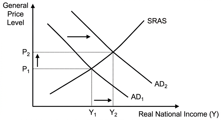
As AD shifts right from AD1 to AD2, the equilibrium level of real national income (Y) rises from Y1 to Y2, generating economic growth. This increase in output leads to derived demand for labour, reducing demand-deficient unemployment. The size of the effect depends on the multiplier: the initial injection of net exports leads to further rounds of spending, amplifying the impact on national income.
Effect on Inflation
The rise in AD puts upward pressure on the general price level, as shown by the movement from P1 to P2 on the diagram. More significantly, the increase in the domestic currency price of imported raw materials and intermediate goods raises firms' costs of production. This cost-push inflation shifts the short-run aggregate supply (SRAS) curve leftwards, further raising the price level and potentially offsetting some of the output gain. The overall effect on inflation is therefore likely to be negative (higher inflation).
Trade-offs and Conflicts
The analysis reveals a clear policy conflict. A falling exchange rate can boost growth and employment (helping achieve those aims) but at the cost of higher inflation (hindering the price stability aim). The effect on the balance of payments is ambiguous in the short run (J-curve) but positive in the long run if the Marshall-Lerner condition holds.
Evaluation
The net effect on the achievement of macroeconomic aims depends on several factors:
- Elasticities: The Marshall-Lerner condition is crucial. If export and import demand are price inelastic (common for primary commodities or countries with few substitutes), the current account may not improve, and the growth stimulus will be weak.
- Supply-side capacity: If the economy is already at or near full capacity (a positive output gap), the increase in AD will mainly cause inflation rather than growth. The SRAS curve will be steep, and the output gain minimal. If there is spare capacity (a negative output gap), the growth effect dominates.
- Pass-through to inflation: The extent to which higher import costs are passed on to consumers depends on the degree of competition in domestic markets. In a highly competitive market, firms may absorb some of the cost increase, limiting inflation.
- Debt servicing: If the country has significant foreign-currency-denominated debt, a depreciation increases the domestic currency cost of servicing that debt, potentially causing a financial crisis that outweighs any trade benefits.
- Time horizon: The J-curve means the short-run effect on the current account is negative, while the long-run effect may be positive. Similarly, the inflationary effect is immediate, while the growth effect may take time to materialise as export volumes adjust.
Conclusion
A fall in the exchange rate is not a straightforward policy tool. It can help achieve growth and employment aims when the economy has spare capacity and demand is elastic, but it simultaneously worsens inflation. The effect on the balance of payments is positive only in the long run and only if the Marshall-Lerner condition is satisfied. The net outcome is therefore conditional: a depreciation is likely to be beneficial for a country with a large output gap and elastic trade, but harmful for a country at full capacity with inelastic trade and high foreign-currency debt. It is not a universal solution to macroeconomic problems.
A fall in the exchange rate can boost economic growth and employment by increasing net exports, but it simultaneously raises inflation through higher import costs. The effect on the balance of payments is positive only in the long run if the Marshall-Lerner condition holds, and is negative in the short run due to the J-curve. The net benefit depends critically on the economy's supply-side capacity, the price elasticities of trade, and the currency denomination of its debt. It is not a universal solution and involves significant trade-offs.
Background Concept
This question tests your understanding of the exchange rate as a macroeconomic variable and its linkages to a country's key objectives: economic growth, price stability (low inflation), a sustainable balance of payments, and full employment. A fall in the exchange rate (depreciation/devaluation) is a change in the external value of the currency. It has two immediate price effects: exports become cheaper for foreign buyers, and imports become more expensive for domestic buyers. These price changes then trigger volume changes, which feed into aggregate demand (AD) and aggregate supply (AS), affecting national income, employment, and the price level.
Key theoretical tools you must deploy:
- AD/AS analysis: To show the effect on real output and the price level.
- The multiplier: To show how an initial change in net exports is amplified through the circular flow.
- The Marshall-Lerner condition: The condition under which a depreciation actually improves the current account (PEDx + PEDm > 1).
- The J-curve: The time-path of the current account following a depreciation, which worsens in the short run before improving in the long run.
- Cost-push inflation: The mechanism by which higher import prices raise domestic costs and shift SRAS leftwards.
Understanding the Question
The question asks you to "Evaluate the effect of a fall in the exchange rate on the achievement of the macroeconomic aims of a country." This is a classic 20-mark Paper 4 essay. The command word "Evaluate" demands a two-sided, developed analysis followed by a justified conclusion. The question does not specify which macroeconomic aims, so you must select at least two (ideally three or four) and analyse the effect on each. The top band (11-14 marks for AO1/AO2) requires "detailed knowledge and understanding," "fully developed" explanations, and the accurate use of analytical tools like diagrams that are "fully explained." The top band for evaluation (4-6 marks) requires a "justified conclusion or judgement that addresses the specific requirements of the question" with "developed, reasoned and well-supported evaluative comment(s)."
You must not simply describe what happens. You must analyse the chains of causation and then evaluate the conditions under which the effects are strong or weak, beneficial or harmful.
Approach
- Define the key term: Start by defining a fall in the exchange rate (depreciation/devaluation) and listing the main macroeconomic aims (growth, low inflation, balance of payments equilibrium, full employment).
- Analyse the effect on the Balance of Payments: This is the most direct effect. Build the chain: fall in ER -> exports cheaper, imports dearer -> if PEDx + PEDm > 1, volume changes outweigh price changes -> current account improves. But introduce the J-curve for the short-run complication.
- Analyse the effect on Economic Growth and Employment: The change in net exports (X-M) is a component of AD. Use an AD/AS diagram. Show AD shifting right. Explain the multiplier effect. Link higher output to derived demand for labour and lower unemployment.
- Analyse the effect on Inflation: Two channels: (a) demand-pull from higher AD, and (b) cost-push from higher import prices. Explain that the SRAS may shift left, creating stagflationary pressure.
- Identify the trade-off: The analysis reveals a conflict between growth/employment (positive) and inflation (negative). This is the core of the evaluation.
- Evaluate: Weigh the factors that determine the net outcome: elasticities, spare capacity, pass-through, debt denomination, time horizon. This is where you show depth.
- Conclude: Provide a justified judgement that answers the question directly. Do not sit on the fence. State the conditions under which the fall is beneficial or harmful.
Step-by-Step Reasoning
Step 1: Define and set the scene.
A fall in the exchange rate means the domestic currency buys fewer units of foreign currency. For example, if the US dollar falls from $1 = €0.90 to $1 = €0.80, US exports to the Eurozone become 12.5% cheaper for Eurozone buyers, while Eurozone imports to the US become 12.5% more expensive for US buyers. The macroeconomic aims typically include: (i) a sustainable balance of payments on current account, (ii) stable prices (low inflation), (iii) economic growth, and (iv) full employment.
Step 2: Effect on the Balance of Payments.
- Price effect: Exports become cheaper in foreign currency, so the volume of exports demanded should rise. Imports become dearer in domestic currency, so the volume of imports demanded should fall.
- Volume effect: The change in the value of the current account depends on the price elasticities of demand for exports and imports. The Marshall-Lerner condition states that a depreciation will improve the current account if PEDx + PEDm > 1. If the sum is less than 1, the current account worsens.
- J-curve: In the very short run, contracts are already in place, and demand is inelastic. The immediate effect is that the import bill rises (because the same volume of imports now costs more in domestic currency) while export revenue may not yet have risen (because volumes have not adjusted). Hence, the current account initially worsens. Over time, as volumes adjust, it improves. This creates a J-shaped time path.
Step 3: Effect on Economic Growth and Employment.
- The improvement in net exports (X-M) is an injection into the circular flow of income. It increases aggregate demand (AD).
- Diagram: Draw an AD/AS diagram. Label the vertical axis "General Price Level" and the horizontal axis "Real National Income (Y)". Draw a downward-sloping AD1 curve and an upward-sloping SRAS curve. The initial equilibrium is at Y1 and P1. The increase in net exports shifts AD rightwards to AD2. The new equilibrium is at Y2 and P2. Real national income rises from Y1 to Y2, representing economic growth. The price level rises from P1 to P2.
- Multiplier effect: The initial increase in AD (from the rise in X-M) leads to higher incomes, which leads to higher consumption, which leads to further increases in AD. The total change in national income = initial change in AD x the multiplier (k = 1/(1-MPC)).
- Employment: As firms increase output to meet the higher demand, they hire more workers. This reduces demand-deficient (cyclical) unemployment.
Step 4: Effect on Inflation.
- Demand-pull inflation: The rightward shift of AD, as shown on the diagram, puts upward pressure on the price level. This is demand-pull inflation.
- Cost-push inflation: More significantly, the rise in the domestic price of imported raw materials, components, and fuel increases firms' costs of production. This shifts the short-run aggregate supply (SRAS) curve leftwards. The combined effect of AD shifting right and SRAS shifting left is a higher price level (more inflation) and an ambiguous effect on real output. The leftward SRAS shift could partially or fully offset the output gain from the AD shift. This is a classic stagflationary scenario.
Step 5: Identify the policy conflict.
The analysis shows a clear trade-off. The fall in the exchange rate helps achieve the aims of economic growth and full employment (assuming spare capacity) but hinders the aim of price stability. The effect on the balance of payments is positive in the long run (if M-L holds) but negative in the short run. The government cannot simultaneously achieve all aims through this single policy.
Step 6: Evaluation (the two-sided weighing).
This is where you earn the AO3 marks. You must go beyond the basic analysis and discuss the conditions that determine the strength and direction of the effects.
- Elasticities (Marshall-Lerner): This is the most critical factor. For a developing country exporting primary commodities (e.g., coffee, copper) with few substitutes, PEDx is likely to be low. Similarly, if the country imports essential goods (e.g., oil, machinery) with no domestic substitutes, PEDm is low. In such cases, the Marshall-Lerner condition may not hold, and the depreciation could worsen the current account, failing to achieve the balance of payments aim.
- Supply-side capacity: If the economy is operating at or near full capacity (a positive output gap), the SRAS curve is steep. An increase in AD will mainly cause inflation, with very little increase in real output. The growth and employment benefits will be minimal. Conversely, if there is a large negative output gap (e.g., in a recession), the SRAS curve is relatively flat, and the same increase in AD will generate significant growth with only a modest rise in inflation.
- Pass-through to inflation: The extent to which higher import costs feed through to consumer prices depends on market structure. In a highly competitive retail sector, firms may absorb some of the cost increase by reducing their profit margins, limiting the inflationary impact. In a less competitive market, firms may pass on the full cost increase.
- Foreign-currency debt: Many developing countries borrow in foreign currencies (e.g., US dollars). A depreciation of their domestic currency increases the domestic currency value of their debt, making it more expensive to service. This can lead to a debt crisis, which would severely harm growth and employment, potentially outweighing any trade benefits.
- Time horizon: The J-curve means the short-run effect on the current account is negative. A government with a short-term focus might abandon the policy before the long-run benefits materialise. The inflationary effect is immediate, while the growth effect takes time. This creates a political economy problem.
- Proportion of trade to GDP: For a very open economy (e.g., Singapore), the effect of an exchange rate change on AD and inflation will be large. For a relatively closed economy (e.g., the US), the effect will be smaller.
Step 7: Conclusion.
A justified conclusion must weigh these factors and state a clear judgement. For example: "A fall in the exchange rate is most likely to help achieve the aims of growth and employment when the economy has significant spare capacity and its trade is price-elastic. However, it will always worsen inflation. The effect on the balance of payments is uncertain in the short run and positive only under specific conditions. Therefore, it is not a universally effective policy and its net benefit is highly context-dependent."
Key Takeaways
- A fall in the exchange rate has multiple, interconnected effects on different macroeconomic aims, creating trade-offs.
- The Marshall-Lerner condition and the J-curve are essential for analysing the balance of payments effect.
- An AD/AS diagram is the primary tool for showing the effect on growth and inflation, but it must be fully explained, not just drawn.
- Evaluation requires discussing the conditions (elasticities, spare capacity, debt, time horizon) that determine the net outcome.
- A justified conclusion must answer the specific question and not just summarise both sides.
Common Mistakes
- One-sided answer: Only discussing the benefits (growth, employment) or only the costs (inflation). This forfeits all evaluation marks.
- No diagram or an unexplained diagram: The mark scheme explicitly requires a diagram. Drawing an AD/AS shift without explaining what each curve represents and what the new equilibrium shows will not earn top marks.
- Confusing a movement along a curve with a shift: A change in the exchange rate shifts the AD curve (via net exports), not a movement along it.
- Ignoring the J-curve: Stating that a depreciation always improves the current account immediately is incorrect and shows a lack of depth.
- No conclusion or a vague conclusion: "It depends" is not a conclusion. You must say what it depends on and which way the balance tips under stated conditions.
- Listing many points without development: The top band requires "fully developed" explanations. One well-developed chain of reasoning (e.g., from exchange rate fall to import prices to costs to SRAS shift to inflation) is worth more than three shallow points.
- Ignoring the supply side: Only analysing the demand-side (AD) effects and forgetting that higher import costs shift SRAS leftwards is a significant omission.
Things to Be Careful About
- Label your diagram correctly: Axes must be labelled "General Price Level" and "Real National Income" (or "Real GDP"). Curves must be labelled AD1, AD2, SRAS. Equilibrium points must be marked (Y1, P1; Y2, P2). Show the direction of the shift with an arrow.
- Use economic terminology precisely: "Depreciation" (floating rate) vs "devaluation" (fixed rate). "Current account" not just "balance of payments." "Cost-push inflation" vs "demand-pull inflation."
- Distinguish short run from long run: The J-curve is a short-run phenomenon. The Marshall-Lerner condition applies to the long run. The effect on growth depends on whether the economy is in the short run (with sticky wages) or the long run (with flexible wages).
- Be specific about the multiplier: State the formula and explain the process, but do not invent numbers unless the question provides them.
- Answer the question asked: The question is about the "achievement of the macroeconomic aims." Your analysis must explicitly link each effect back to whether it helps or hinders the achievement of a specific aim. Do not just describe the effects in isolation.
Evaluate whether the presence of multinational companies (MNCs) in low-income countries is always beneficial.
Introduction
A multinational company (MNC) is a firm that operates in more than one country, typically through foreign direct investment (FDI). A low-income country (LIC) is defined by the World Bank as one with a GNI per capita below a certain threshold (e.g. US$1,135 in 2022). This essay evaluates whether the presence of MNCs in LICs is always beneficial, considering both the potential gains and the significant drawbacks.
The case that MNCs are beneficial
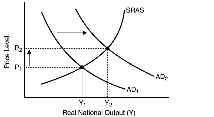
MNCs bring capital, technology, and managerial expertise that LICs lack. This investment increases aggregate demand (AD) in the host economy. For example, an MNC building a factory creates construction jobs and then permanent employment. The rise in employment raises incomes, which increases consumption, further boosting AD. This can be shown with an AD/AS diagram: AD shifts right from AD1 to AD2, increasing real national output from Y1 to Y2 and, if the economy is below full employment, reducing unemployment.
In the long run, MNCs can increase potential output. They invest in infrastructure (roads, ports, power) and train local workers, shifting the long-run aggregate supply (LRAS) curve rightwards and the production possibility curve (PPC) outwards. This raises the economy's trend growth rate. The transfer of technology and management practices can also improve productivity in domestic firms through spillover effects.
MNCs also improve the balance of payments on the capital and financial account through inward FDI. If they export a significant share of output, the current account also improves. The increased supply of foreign exchange from export earnings can strengthen the exchange rate, reducing the cost of imported capital goods.
The case against MNCs being always beneficial
However, the benefits are not automatic or universal. MNCs may crowd out local firms that cannot compete with their scale and technology, leading to deindustrialisation and structural unemployment. Profits are often repatriated rather than reinvested, so the net capital inflow may be smaller than the gross figure suggests.
MNCs can cause negative externalities. They may exploit weak environmental regulations, creating pollution and resource depletion that impose social costs exceeding private benefits. In the extractive sector, the 'Dutch disease' can occur: large inflows of foreign exchange from raw material exports appreciate the real exchange rate, making other export sectors uncompetitive and causing a loss of manufacturing jobs.
There are also governance concerns. MNCs may engage in transfer pricing to avoid tax, depriving the LIC of revenue. Corruption of local officials to secure favourable terms can undermine institutions and distort policy. Cultural disruption and changes in work practices may reduce non-material living standards even if measured GDP rises.
Evaluation
The net effect depends critically on the type of MNC activity, the host country's policies, and the strength of its institutions. MNCs in manufacturing with high local content and strong backward linkages tend to generate more benefits than those in extractive industries with few linkages. A LIC with a skilled workforce, good infrastructure, and effective regulation can capture more of the gains. Conversely, a LIC with weak governance and a narrow resource-based economy may suffer more from the drawbacks.
Conclusion
The presence of MNCs in low-income countries is not always beneficial. While they can bring capital, jobs, technology, and growth, these benefits are conditional on the sector, the host country's policies, and the behaviour of the MNC. In many cases, the costs — including crowding out, environmental damage, Dutch disease, and governance problems — can outweigh the gains. Therefore, the statement that MNCs are always beneficial is false; the outcome is context-dependent and requires careful policy management to maximise net benefits.
The presence of MNCs in low-income countries is not always beneficial; the net effect depends on the sector, host-country policies, and institutional quality, with significant potential costs that can outweigh the gains.
Background Concept
A multinational company (MNC) is a firm that owns or controls production facilities in more than one country, typically through foreign direct investment (FDI). Low-income countries (LICs) are characterised by low GNI per capita, limited capital, low levels of technology, and often weak institutions. The core economic question is whether the net welfare effect of MNC presence is positive — i.e., whether the benefits to the host economy exceed the costs. This involves analysing impacts on aggregate demand and supply, the balance of payments, employment, externalities, and institutional quality.
Understanding the Question
The question asks: "Evaluate whether the presence of multinational companies (MNCs) in low-income countries is always beneficial." The key word is "always" — an absolute claim. The command word "Evaluate" requires a two-sided analysis and a justified conclusion. The top band (AO3) demands a justified conclusion that addresses the specific requirements of the question. The AO1/AO2 top band requires detailed knowledge, fully developed explanations, and accurate use of analytical tools such as diagrams. The question is an undivided 20-mark essay (AO1+AO2 out of 14, AO3 out of 6).
Approach
The essay will first define key terms. Then it will develop the case for MNCs being beneficial, using an AD/AS diagram to show short-run demand-side effects and a PPC/LRAS argument for long-run supply-side effects. It will then develop the counter-case, covering crowding out, profit repatriation, negative externalities, Dutch disease, and governance issues. Evaluation will weigh these against each other using criteria such as sector type, host-country policies, and institutional strength. The conclusion will reject the absolute claim and state that benefits are conditional.
Step-by-Step Reasoning
Step 1: Definitions
- MNC: a firm with operations in multiple countries, usually via FDI.
- LIC: a country with low GNI per capita (e.g., < US$1,135).
Step 2: The beneficial case
- MNCs bring capital, technology, and management skills that are scarce in LICs.
- This investment increases AD: construction jobs, then permanent employment, then higher consumption. The multiplier effect amplifies the initial spending.
- AD/AS diagram: AD shifts right, increasing real output and reducing unemployment (if below full employment).
- Long-run: MNCs invest in infrastructure and training, shifting LRAS right and PPC outward. This raises potential growth.
- Balance of payments: inward FDI improves the capital account; exports improve the current account. The increased supply of foreign exchange can strengthen the exchange rate, reducing import costs.
Step 3: The counter-case
- Crowding out: MNCs may outcompete local firms, leading to deindustrialisation and structural unemployment.
- Profit repatriation: net capital inflow may be small if profits are sent home.
- Negative externalities: pollution, resource depletion, and environmental damage impose social costs.
- Dutch disease: large foreign exchange inflows from resource exports appreciate the real exchange rate, harming other export sectors and causing job losses.
- Governance issues: transfer pricing reduces tax revenue; corruption distorts policy; cultural disruption reduces non-material living standards.
Step 4: Evaluation
- The net effect depends on:
- Sector: manufacturing with linkages > extractive industries.
- Host-country policies: strong regulation, skilled workforce, good infrastructure capture more gains.
- MNC behaviour: reinvestment vs. repatriation, environmental standards, tax compliance.
- A LIC with weak institutions may suffer more from the drawbacks.
Step 5: Conclusion
- The statement that MNCs are "always beneficial" is false. Benefits are conditional and context-dependent. In many cases, costs can outweigh benefits. Therefore, the presence of MNCs is not always beneficial.
Key Takeaways
- MNCs can bring significant benefits to LICs, but these are not automatic.
- The net effect depends on the sector, host-country policies, and MNC behaviour.
- Absolute claims ("always", "never") in economics are rarely correct and must be challenged with counter-examples.
- Evaluation requires weighing costs and benefits using explicit criteria and reaching a justified conclusion.
Common Mistakes
- One-sided answer: only listing benefits or only listing costs. This forfeits all AO3 marks.
- No conclusion or a vague conclusion (e.g., "it depends" without saying on what).
- No diagram or an unexplained diagram. The top band requires diagrams to be fully explained.
- Confusing correlation with causation: assuming MNC presence causes growth without considering other factors.
- Ignoring the specific context of LICs: applying analysis relevant to developed countries without adjustment.
Things to Be Careful About
- Label all axes and curves in the diagram. Explain the shift and its effect on equilibrium.
- Use the extract's evidence if provided (none here, but in a data-response question, always cite figures).
- Distinguish between short-run demand-side effects and long-run supply-side effects.
- Ensure the conclusion is justified, not just a summary. State which side is stronger and why.
- Avoid over-generalising: the answer should acknowledge that outcomes vary by country and sector.