Economics 9708/34 — October/November 2025
Cambridge A-Level · A Level Multiple Choice · answer key with instant marking and worked solutions
Topics Equity, Poverty and Redistribution · Economic Growth and Sustainability · Government Policies to Correct Market Failure · Demand for and Supply of Labour · Wage Determination and Labour Market Intervention · Money and Banking · +15 more
Tap an option under each question to check it — your score builds as you go.
What will act as a barrier to collusion between firms?
Options
A an ability to detect price cuts by rivals
B the abolition of anti-trust measures
C the existence of a small number of firms in the industry
D unstable demand conditions for products
Answer
Collusion between firms is more likely to succeed when market conditions are stable and predictable. Unstable demand conditions (option D) make it difficult for firms to agree on output levels and prices, and increase the incentive to cheat on any agreement, thus acting as a barrier to collusion.
Option A is incorrect because the ability to detect price cuts actually facilitates collusion by making cheating easier to identify and punish. Option B is incorrect because the abolition of anti-trust measures removes legal barriers to collusion, making it easier. Option C is incorrect because a small number of firms typically makes collusion easier to coordinate and monitor.
Therefore, the correct answer is D.
D
Background Concept
Collusion occurs when firms in an oligopolistic market cooperate to restrict output and raise prices, often to increase joint profits. Successful collusion requires firms to agree on a common price or output level and to monitor each other to prevent cheating. The Prisoner's Dilemma illustrates the tension: each firm has an incentive to cheat on the agreement to gain market share, but if all cheat, they all end up worse off. Factors that make collusion more difficult include unstable demand, many firms, product differentiation, and weak legal enforcement.
Understanding the Question
The question asks: "What will act as a barrier to collusion between firms?" It is a multiple-choice question with four options. The correct answer is the factor that makes collusion harder to achieve or sustain. The other options are factors that would actually facilitate collusion.
Approach
Evaluate each option in turn, considering whether it helps or hinders collusion. Use economic reasoning about the conditions necessary for collusion to be effective: stable market conditions, ability to detect cheating, few firms, and absence of legal prohibitions.
Step-by-Step Reasoning
- Option A: an ability to detect price cuts by rivals. If firms can easily detect when a rival cuts price, they can quickly retaliate, which deters cheating. This actually supports collusion, not hinders it. So A is not a barrier.
- Option B: the abolition of anti-trust measures. Anti-trust laws (e.g., competition laws) prohibit collusion. Abolishing them removes legal penalties, making collusion easier. So B is not a barrier.
- Option C: the existence of a small number of firms in the industry. A small number of firms makes coordination and monitoring easier, facilitating collusion. So C is not a barrier.
- Option D: unstable demand conditions for products. When demand is unstable, it is hard to agree on a common price or output because the optimal level changes frequently. Moreover, firms may have different expectations about future demand, leading to disagreements. Unstable demand also increases the temptation to cheat to capture sales during booms or to avoid losses during slumps. Thus, unstable demand acts as a barrier to collusion.
Therefore, D is the correct answer.
Key Takeaways
- Collusion is easier when market conditions are stable, there are few firms, and cheating can be detected and punished.
- Unstable demand undermines the basis for agreement and increases incentives to cheat.
- Legal prohibitions (anti-trust) are a barrier to collusion, so their removal would facilitate it.
Common Mistakes
- Confusing factors that help collusion with those that hinder it. For example, thinking that a small number of firms makes collusion harder (it actually makes it easier).
- Overlooking the role of demand stability: students may focus only on supply-side factors.
Things to Be Careful About
- Read each option carefully and think about its effect on the ability to coordinate and sustain collusion.
- Remember that collusion is illegal in many countries, so legal factors matter.
- The question asks for a barrier, so choose the option that makes collusion more difficult.
The diagram shows two indifference curves.
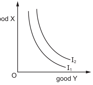
What do indifference curves indicate?
Options
A Consumers get more satisfaction on curve I1 from consuming more of X and less of Y.
B Consumers get more satisfaction on curve I2 from consuming less of X and more of Y.
C Each point on the curve represents the marginal rate of substitution of good X for good Y.
D Movement from I1 to I2 cannot be made unless the indifference curves cross.
Reasoning
An indifference curve maps all combinations of two goods that yield the same level of consumer utility (satisfaction). The marginal rate of substitution (MRS) of good X for good Y at any point on the curve is the quantity of good Y the consumer is willing to sacrifice to obtain one additional unit of good X, while remaining on the same indifference curve (i.e., maintaining the same utility level). By definition, every point on an indifference curve corresponds to a specific MRS of X for Y for that consumption bundle.
Answer
C
C
Background Concept
Indifference curves are a core tool in ordinal utility theory, used to model consumer preferences. They rely on key assumptions: consumers are rational, they can rank preferences between bundles of two goods (ordinal utility, not cardinal), they prefer more of a good to less (non-satiation), their preferences are transitive (if they prefer A to B and B to C, they prefer A to C), and they are willing to substitute between the two goods at a diminishing rate (diminishing marginal rate of substitution, MRS).
Each individual indifference curve represents all combinations of the two goods that give the consumer exactly the same level of utility. Curves further from the origin represent higher utility levels, as they contain bundles with more of at least one good. The MRS of X for Y at any point on the curve is the absolute value of the curve's slope at that point: it measures how much Y the consumer will give up to get one extra unit of X, while staying on the same curve (so utility does not change). A key property of indifference curves is that they cannot cross, as this would violate the transitivity of preferences. They are also always convex to the origin, due to the diminishing MRS.
Understanding the Question
The question presents a standard indifference curve diagram with two curves: I1 (closer to the origin, lower utility) and I2 (further from the origin, higher utility), with good X on the vertical axis and good Y on the horizontal. It asks which statement correctly describes what indifference curves indicate. This is a 1-mark multiple-choice question testing basic recall of indifference curve definitions and properties.
Approach
First, restate the core definition and properties of indifference curves, then evaluate each of the four options against these properties to identify the only correct statement.
Step-by-Step Reasoning
- First, list the key relevant properties of indifference curves:
- All points on a single indifference curve give the consumer identical utility. Moving along the curve (more of one good, less of the other) keeps utility constant.
- Higher indifference curves (further from the origin) represent higher utility, so any point on I2 gives greater satisfaction than any point on I1.
- The MRS of X for Y at any point on the curve is the trade-off the consumer is willing to make between the two goods at that bundle, represented by the slope of the curve at that point.
- Indifference curves never cross, as crossing would imply inconsistent (non-transitive) preferences.
- Evaluate each option:
- Option A: Claims consumers get more satisfaction on I1 from consuming more X and less Y. This is false: all points on I1 give the same level of satisfaction. Moving along I1 to more X and less Y does not increase utility, it keeps it constant.
- Option B: Claims consumers get more satisfaction on I2 from consuming less X and more Y. This is false: all points on I2 give the same (higher than I1) level of satisfaction. Moving along I2 to less X and more Y keeps utility constant on I2, it does not increase satisfaction further.
- Option C: Claims each point on the curve represents the marginal rate of substitution of good X for good Y. This is true: by definition, the MRS at a point on the indifference curve is the exact trade-off between X and Y the consumer is willing to make at that consumption bundle, which is what the point represents.
- Option D: Claims movement from I1 to I2 cannot be made unless the indifference curves cross. This is false: I2 is a separate, higher indifference curve, so movement from I1 to I2 represents a gain in utility (the consumer is better off). Indifference curves never cross, so this movement does not require crossing curves at all.
- The only correct statement is Option C.
Key Takeaways
- Indifference curves represent bundles of two goods that give the same level of consumer utility; higher curves (further from the origin) mean higher utility.
- The marginal rate of substitution (MRS) is the trade-off between two goods that keeps utility constant, and is represented by the slope of the indifference curve at each point.
- Indifference curves cannot cross, as this would violate the transitivity of consumer preferences.
- Movement along an indifference curve keeps utility constant; movement to a higher curve increases utility, movement to a lower curve decreases utility.
Common Mistakes
- Confusing movement along an indifference curve (constant utility) with movement between curves (changing utility). For example, assuming that moving to more X and less Y along I1 increases satisfaction, when it actually keeps it the same.
- Assuming that moving along a higher indifference curve increases satisfaction, rather than keeping it at the same higher level.
- Forgetting that the MRS is specific to a single point on the curve, representing the trade-off at that exact consumption bundle.
Things to Be Careful About
- Utility in indifference curve analysis is ordinal (ranked) not cardinal: we only compare whether one bundle is better/worse than another, or whether two bundles are equally preferred, we do not measure exact utility values.
- The MRS is technically negative (since the curve slopes downwards), but it is almost always referred to by its absolute value when describing the trade-off between goods.
- The convex shape of indifference curves comes from the diminishing MRS: as a consumer has more of X and less of Y, they are willing to give up less Y to get an extra unit of X, because X is becoming relatively more abundant and Y relatively scarcer.
What is an example of forward vertical integration?
Options
A A firm manufacturing computers merges with a firm that manufactures furniture.
B A firm manufacturing computers merges with a firm that manufactures silicon chips for computers.
C A firm manufacturing computers merges with a retail outlet that sells computers.
D A firm manufacturing computers merges with another firm that also manufactures computers.
Answer
Forward vertical integration occurs when a firm merges with or takes over another firm that is closer to the final consumer in the supply chain. A computer manufacturer merging with a retail outlet that sells computers is an example of forward vertical integration, as the manufacturer is moving forward towards the consumer.
Answer
C
C
Background Concept
Vertical integration is a type of external growth where a firm merges with or takes over another firm operating at a different stage of the same industry's supply chain. The supply chain traces the journey of a product from raw material to final consumer. There are two directions of vertical integration:
- Backward (upstream) vertical integration: The firm merges with a supplier of its inputs, moving backwards in the supply chain. For example, a car manufacturer merging with a steel producer.
- Forward (downstream) vertical integration: The firm merges with a business closer to the final consumer, such as a distributor or retailer, moving forwards in the supply chain.
This is distinct from:
- Horizontal integration: A merger between two firms at the same stage of production in the same industry (e.g., two car manufacturers merging).
- Conglomerate integration: A merger between firms in unrelated industries.
Understanding the Question
The question asks you to identify which of the four scenarios is an example of forward vertical integration. The key is to identify the computer manufacturer's position in its supply chain and then determine which of the other firms is closer to the final consumer. The correct answer will be the one where the computer manufacturer moves forward towards the end-user.
Approach
- Define forward vertical integration: A merger with a firm closer to the final consumer.
- Analyze each option: Determine the position of the second firm relative to the computer manufacturer in the supply chain.
- Option A: Furniture is unrelated to computers. This is conglomerate integration.
- Option B: Silicon chips are an input for computers. This is backward vertical integration.
- Option C: A retail outlet sells the finished computer to the consumer. This is forward vertical integration.
- Option D: Another computer manufacturer is at the same stage. This is horizontal integration.
- Select the correct option: The option that matches the definition of forward vertical integration.
Step-by-Step Reasoning
- Identify the base firm: The firm in question is a computer manufacturer. Its position in the supply chain is the assembly and production of finished computers.
- Analyze Option A: A furniture manufacturer is in a completely different industry. A merger between a computer manufacturer and a furniture manufacturer is a conglomerate merger, not a vertical one. Therefore, A is incorrect.
- Analyze Option B: Silicon chips are a key component (input) used in manufacturing computers. A firm that manufactures silicon chips is a supplier to the computer manufacturer. A merger with a supplier is backward vertical integration, not forward. Therefore, B is incorrect.
- Analyze Option C: A retail outlet that sells computers is the next step in the supply chain after the computer is manufactured. The retail outlet is the point of sale to the final consumer. A merger with this retail outlet is a move forward towards the consumer. This perfectly matches the definition of forward vertical integration. Therefore, C is correct.
- Analyze Option D: Another firm that also manufactures computers is at the same stage of production. A merger between two firms at the same stage is horizontal integration. Therefore, D is incorrect.
Key Takeaways
- Supply Chain Direction: The key to distinguishing forward from backward vertical integration is to think about the flow of the product from raw materials to the consumer. Forward is towards the consumer; backward is towards the raw materials.
- Distinguishing Integration Types: Be able to clearly differentiate between horizontal (same stage), vertical (different stages in the same chain), and conglomerate (different industries) integration.
- Application: This question tests the ability to apply a theoretical definition to a practical, real-world business scenario.
Common Mistakes
- Confusing Forward and Backward: The most common mistake is mixing up the two directions. Students might think that merging with a supplier (getting inputs) is 'forward' because it's a step in the production process, but 'forward' is defined by proximity to the final consumer, not the production sequence.
- Confusing Vertical and Horizontal: A student might see two firms in the same broad industry (computers) and incorrectly assume it's vertical integration, without checking if they are at different stages of the supply chain.
Things to Be Careful About
- Read the Direction: Always note whether the question asks for 'forward' or 'backward' vertical integration.
- Define the Supply Chain: Before answering, mentally map out the simple supply chain for the product in question (e.g., raw materials -> component manufacturer -> assembler -> wholesaler -> retailer -> consumer). This makes the direction of integration clear.
- Focus on the Relationship: The key is the relationship between the two merging firms in the production and distribution process, not just the industry they are in.
The diagram shows positive and negative externalities of production and consumption.
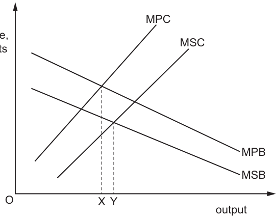
Which row shows the correct combination of production and consumption externality when economic welfare is maximised?
Options
| position of economic welfare | production externality | consumption externality | |
|---|---|---|---|
| A | X | negative | negative |
| B | Y | positive | negative |
| C | X | negative | positive |
| D | Y | positive | positive |
Reasoning
Economic welfare is maximised at the allocatively efficient output where marginal social cost (MSC) equals marginal social benefit (MSB). The diagram shows this occurs at output Y, not X (which is the private market equilibrium where MPC = MPB).
To classify the externalities:
- Production externality: The MSC curve lies below the MPC curve, meaning social cost is lower than private cost. This indicates a positive production externality (external benefits from production).
- Consumption externality: The MSB curve lies below the MPB curve, meaning social benefit is lower than private benefit. This indicates a negative consumption externality (external costs from consumption).
This combination matches row B.
Answer
B
B
Background Concept
Externalities are costs or benefits of economic activity that affect third parties not directly involved in the transaction, and are not reflected in market prices. They are classified as positive (external benefits) or negative (external costs), and can arise from production or consumption.
- Production externalities: occur when a firm's production imposes costs or benefits on third parties. Marginal private cost (MPC) is the cost to the firm of producing one more unit. Marginal social cost (MSC) is the total cost to society of that unit, equal to MPC plus any marginal external cost (MEC) of production. If MSC > MPC, there is a negative production externality (external costs, e.g. pollution from a factory). If MSC < MPC, there is a positive production externality (external benefits, e.g. a firm's research that spills over to other industries).
- Consumption externalities: occur when a consumer's consumption imposes costs or benefits on third parties. Marginal private benefit (MPB) is the benefit to the consumer of consuming one more unit. Marginal social benefit (MSB) is the total benefit to society of that unit, equal to MPB plus any marginal external benefit (MEB) of consumption. If MSB > MPB, there is a positive consumption externality (external benefits, e.g. education reducing crime). If MSB < MPB, there is a negative consumption externality (external costs, e.g. passive smoking from someone else's cigarette consumption).
- Economic welfare maximisation: this occurs at the allocatively efficient output level, where the marginal benefit to society of the last unit produced equals the marginal cost to society of producing it: MSC = MSB. At this point, there is no deadweight welfare loss, and total economic surplus (consumer + producer surplus plus any external benefits minus external costs) is maximised. The unregulated private market equilibrium occurs where MPC = MPB, which will only coincide with the social optimum if there are no externalities.
Understanding the Question
The question presents a diagram with four curves (MPC, MSC, MPB, MSB) and two output levels: X (where MPC = MPB, the private market equilibrium) and Y (where MSC = MSB, the social optimum). It asks which row correctly identifies the welfare-maximising output level, plus the type of production and consumption externality present. The task requires applying knowledge of externality classification and the condition for maximum economic welfare to the labelled diagram.
Approach
- First, identify the welfare-maximising output: recall that economic welfare is maximised where MSC = MSB, which the diagram states is output Y, so eliminate options A and C which cite X.
- Next, identify the production externality: compare the positions of MPC and MSC. If MSC is below MPC, social cost is lower than private cost, indicating a positive production externality. If MSC is above MPC, it is a negative production externality.
- Then identify the consumption externality: compare the positions of MPB and MSB. If MSB is below MPB, social benefit is lower than private benefit, indicating a negative consumption externality. If MSB is above MPB, it is a positive consumption externality.
- Match these findings to the remaining options (B and D) to select the correct row.
Step-by-Step Reasoning
- Identify the welfare-maximising output: The condition for maximum economic welfare (allocative efficiency) is that the marginal social cost of the last unit produced equals the marginal social benefit gained from consuming it: MSC = MSB. The diagram explicitly labels output Y as the point where MSC = MSB, so Y is the welfare-maximising position. This immediately rules out options A and C, which incorrectly state the welfare-maximising position is X (the private market equilibrium where MPC = MPB, which only maximises private welfare, not total social welfare when externalities exist).
- Classify the production externality: Compare the MPC and MSC curves. The MPC curve is steeper and lies above the MSC curve at all output levels (evident from the diagram, where at output Y, the MPC curve is above the MSC curve). This means that for any given level of output, the marginal private cost to the firm is higher than the marginal social cost to society. The difference between MPC and MSC is the marginal external cost (MEC) of production: MSC = MPC - MEC, so MEC is positive, meaning production generates external benefits for third parties. This is a positive production externality.
- Classify the consumption externality: Compare the MPB and MSB curves. The MPB curve lies above the MSB curve at all output levels (evident from the diagram, where MPB is the upper downward-sloping curve, MSB is the lower one). This means that for any given level of output, the marginal private benefit to the consumer is higher than the marginal social benefit to society. The difference between MPB and MSB is the marginal external cost (MEC) of consumption: MSB = MPB - MEC, so MEC is positive, meaning consumption imposes external costs on third parties. This is a negative consumption externality, which eliminates option D (which incorrectly states the consumption externality is positive).
- Match to the options: The correct combination is welfare-maximising position Y, positive production externality, negative consumption externality, which is row B.
Key Takeaways
- The condition for maximum economic welfare (allocative efficiency) is MSC = MSB, not the private market equilibrium MPC = MPB.
- A positive production externality exists when MSC < MPC (social cost is lower than private cost, due to external benefits from production).
- A negative consumption externality exists when MSB < MPB (social benefit is lower than private benefit, due to external costs from consumption).
- When classifying externalities, always compare the social curve (MSC/MSB) to the private curve (MPC/MPB) to identify the direction of the externality.
Common Mistakes
- Confusing the private equilibrium (X, MPC=MPB) with the social optimum (Y, MSC=MSB): X only maximises private welfare, not total social welfare when externalities are present.
- Mixing up the direction of externalities: a negative externality means the social curve is worse (higher cost, lower benefit) than the private curve, while a positive externality means the social curve is better (lower cost, higher benefit) than the private curve.
- Misreading the diagram's curve positions: assuming MSC is always above MPC (which is only true for negative production externalities) or MSB is always above MPB (only true for positive consumption externalities), without checking the actual diagram.
- Forgetting that the question asks for the combination at the welfare-maximising position, not the private equilibrium.
Things to Be Careful About
- Always check the relative positions of the curves in the specific diagram provided, rather than relying on default assumptions about externalities (e.g. pollution is a negative production externality, but not all production externalities are negative).
- Confirm the axis labels and curve labels: upward-sloping curves are cost curves (MPC, MSC), downward-sloping are benefit curves (MPB, MSB).
- Remember that the welfare-maximising output is always where the social marginal cost equals social marginal benefit, regardless of the type of externality.
- When matching to options, eliminate rows with the wrong welfare position first, then check the externality types to avoid confusion between similar options.
A firm has fixed costs of $300 and can produce two units per hour. Its total variable costs are $200 for one unit and $300 for two units.
Which cost will fall by the lowest amount when the second unit is produced?
Options
A average fixed cost
B average total cost
C average variable cost
D marginal cost
Working
For 1 unit:
- TFC = $300
- TVC = $200
- TC = TFC + TVC = $300 + $200 = $500
- AFC = TFC / Q = $300 / 1 = $300
- AVC = TVC / Q = $200 / 1 = $200
- ATC = TC / Q = $500 / 1 = $500
- MC = change in TC = $500 - $0 = $500 (or change in TVC = $200 - $0 = $200)
For 2 units:
- TFC = $300
- TVC = $300
- TC = $300 + $300 = $600
- AFC = $300 / 2 = $150
- AVC = $300 / 2 = $150
- ATC = $600 / 2 = $300
- MC = change in TC = $600 - $500 = $100 (or change in TVC = $300 - $200 = $100)
Change when second unit is produced:
- AFC falls by $300 - $150 = $150
- ATC falls by $500 - $300 = $200
- AVC falls by $200 - $150 = $50
- MC falls by $500 - $100 = $400 (but note MC is not a 'fall' in the same sense; it is the cost of the marginal unit, which is lower for the second unit than the first)
The smallest fall is $50 for average variable cost.
Answer
C
C
Background Concept
This question tests your understanding of the different cost concepts a firm faces in the short run. The key distinction is between fixed costs (which do not change with output) and variable costs (which do change with output). From these, we derive total cost (TC), average fixed cost (AFC), average variable cost (AVC), average total cost (ATC), and marginal cost (MC).
- Total Fixed Cost (TFC): Constant at all output levels in the short run. Here, $300.
- Total Variable Cost (TVC): Increases as output rises. Given as $200 for 1 unit, $300 for 2 units.
- Total Cost (TC): TFC + TVC.
- Average Fixed Cost (AFC): TFC / Q. Falls continuously as output rises because the same fixed cost is spread over more units.
- Average Variable Cost (AVC): TVC / Q. Can fall, rise, or stay constant depending on the production function.
- Average Total Cost (ATC): TC / Q. The sum of AFC and AVC.
- Marginal Cost (MC): The change in total cost (or total variable cost) when one more unit is produced.
The question asks which cost falls by the lowest amount when the second unit is produced. This requires calculating each cost at 1 unit and at 2 units, then finding the difference.
Understanding the Question
The question gives:
- Fixed costs = $300 (constant)
- Output per hour = 2 units (so we consider Q = 1 and Q = 2)
- TVC at Q = 1: $200
- TVC at Q = 2: $300
We are asked: "Which cost will fall by the lowest amount when the second unit is produced?" The options are four different cost measures: AFC, ATC, AVC, and MC. Note that MC is the cost of producing the next unit, so it is not a 'fall' in the same way as the averages; we compare the MC of the first unit ($500) with the MC of the second unit ($100) — a fall of $400. But the question is about the amount each cost falls, so we calculate the absolute change.
Approach
- Calculate TC, AFC, AVC, ATC, and MC for Q = 1 and Q = 2.
- Compute the change in each cost measure when output increases from 1 to 2.
- Identify which change is the smallest (lowest absolute fall).
Step-by-Step Reasoning
Step 1: Costs at Q = 1
- TFC = $300
- TVC = $200
- TC = $300 + $200 = $500
- AFC = $300 / 1 = $300
- AVC = $200 / 1 = $200
- ATC = $500 / 1 = $500
- MC (from 0 to 1 unit) = change in TC = $500 - $0 = $500 (or change in TVC = $200 - $0 = $200; both give the same MC because fixed costs don't change)
Step 2: Costs at Q = 2
- TFC = $300 (unchanged)
- TVC = $300
- TC = $300 + $300 = $600
- AFC = $300 / 2 = $150
- AVC = $300 / 2 = $150
- ATC = $600 / 2 = $300
- MC (from 1 to 2 units) = change in TC = $600 - $500 = $100 (or change in TVC = $300 - $200 = $100)
Step 3: Calculate the fall in each cost
- AFC falls from $300 to $150: a fall of $150.
- ATC falls from $500 to $300: a fall of $200.
- AVC falls from $200 to $150: a fall of $50.
- MC falls from $500 to $100: a fall of $400.
Step 4: Identify the smallest fall
The smallest fall is $50, which is the change in average variable cost (AVC).
Therefore, the correct answer is C.
Key Takeaways
- Always calculate all relevant cost measures from the given data before comparing.
- AFC always falls as output increases, but the amount of the fall depends on the level of fixed costs and the change in output.
- AVC can fall, rise, or stay constant; here it falls because the variable cost per unit decreases from $200 to $150.
- MC is the cost of the marginal unit; it can be very different from average costs.
- The question tests the ability to compute and compare different cost concepts, not just recall definitions.
Common Mistakes
- Confusing average and marginal costs: Some students might think MC is always the lowest cost, but here it falls by the largest amount, not the smallest.
- Forgetting to calculate AFC: AFC always falls, but the amount of the fall is not always the smallest; here it is larger than the fall in AVC.
- Misreading the question: The question asks which cost falls by the lowest amount, not which cost is lowest in absolute terms.
- Incorrect calculation of MC: MC is the change in TC (or TVC) when output increases by one unit. Some might calculate MC as the change in ATC, which is wrong.
Things to Be Careful About
- Always show your working clearly, even for a multiple-choice question, to avoid arithmetic errors.
- Remember that fixed costs are constant in the short run, so AFC falls as output rises.
- MC is not an average; it is the cost of the next unit. Comparing the MC of the first unit with the MC of the second unit gives a change, but the question asks about the fall in each cost measure, so we compare the values at Q=1 and Q=2.
- Double-check which cost measure each option refers to: A is AFC, B is ATC, C is AVC, D is MC.
What is the most likely evidence that an economy has reached a position of Pareto optimality?
Options
A price volatility
B a large current account deficit
C a regressive taxation system
D full employment
Answer
Pareto optimality is a situation where no one can be made better off without making someone else worse off. This is most likely to occur when all resources are fully employed in their most efficient uses. Full employment of resources is a necessary condition for Pareto optimality, as unemployed resources could be used to make someone better off without harming anyone else.
Answer
D
D
Background Concept
Pareto optimality (or Pareto efficiency) is a key concept in welfare economics. It describes a state of allocation of resources in which it is impossible to make any one individual better off without making at least one individual worse off. This is a condition of allocative efficiency. For an economy to be Pareto optimal, several conditions must hold:
- Efficiency in exchange: The marginal rate of substitution (MRS) between any two goods must be equal for all consumers.
- Efficiency in production: The marginal rate of technical substitution (MRTS) between any two inputs must be equal for all producers.
- Efficiency in product mix: The marginal rate of transformation (MRT) between any two goods must equal the MRS for all consumers.
A key prerequisite for achieving these conditions is that all resources are fully employed. If there are unemployed resources (e.g., labour, capital), it is possible to use them to produce more of some goods without reducing the output of others, thereby making someone better off without making anyone worse off. This violates the condition of Pareto optimality.
Understanding the Question
This is a multiple-choice question asking for the 'most likely evidence' that an economy has reached Pareto optimality. It requires you to select the option that is a necessary condition or a strong indicator of this state. The question tests your understanding of what Pareto optimality implies in a real-world macroeconomic context, rather than just its theoretical definition.
Approach
- Recall the definition of Pareto optimality: A state where no one can be made better off without making someone else worse off.
- Analyse each option: Determine whether each option is a necessary condition, a likely consequence, or unrelated to Pareto optimality.
- Eliminate incorrect options: Identify why options A, B, and C are not evidence of Pareto optimality.
- Select the correct option: Confirm why option D is the most likely evidence.
Step-by-Step Reasoning
Let's evaluate each option:
-
Option A: price volatility. Price volatility refers to rapid and unpredictable changes in prices. This is a feature of markets with unstable supply or demand, speculation, or imperfect information. It does not indicate that resources are allocated efficiently. In fact, high volatility can lead to misallocation of resources and uncertainty, which is the opposite of a Pareto optimal state. Therefore, A is incorrect.
-
Option B: a large current account deficit. A current account deficit means a country is importing more goods and services than it is exporting. This is a macroeconomic imbalance. While it can be a sign of a growing economy (importing capital goods), it is not evidence of Pareto optimality. A deficit can exist even when resources are misallocated or underemployed. Pareto optimality is about the efficiency of allocation, not the balance of trade. Therefore, B is incorrect.
-
Option C: a regressive taxation system. A regressive tax system takes a larger percentage of income from low-income earners than from high-income earners. This is a matter of equity (fairness), not efficiency. Pareto optimality is a condition of efficiency, not equity. A regressive tax system could be in place in an economy that is Pareto optimal, but it is not evidence of it. In fact, a regressive tax might create disincentives to work, leading to inefficiency. Therefore, C is incorrect.
-
Option D: full employment. Full employment means that all available labour resources are being used in the most efficient way possible. In a state of full employment, there is no involuntary unemployment. If there were unemployed workers, they could be employed to produce more goods and services, making some people better off (e.g., the newly employed workers and the consumers of the extra output) without making anyone else worse off. This would be a Pareto improvement. Therefore, the absence of such an opportunity (i.e., full employment) is a necessary condition for Pareto optimality. It is the most likely evidence among the options.
Key Takeaways
- Pareto optimality is a state of allocative efficiency where no further Pareto improvements are possible.
- A Pareto improvement is a change that makes at least one person better off without making anyone else worse off.
- Full employment of resources is a necessary condition for Pareto optimality because unemployed resources represent a potential Pareto improvement.
- Pareto optimality is a concept of efficiency, not equity or macroeconomic balance. A Pareto optimal state can be highly unequal.
Common Mistakes
- Confusing Pareto optimality with equity: A common mistake is to think that a Pareto optimal state is 'fair' or 'just'. It is not. It is purely about efficiency. A situation where one person has everything and everyone else has nothing can be Pareto optimal if taking from the rich person makes them worse off.
- Confusing Pareto optimality with full employment of all resources: While full employment of labour is a key condition, Pareto optimality also requires that capital, land, and other resources are fully and efficiently employed. The question asks for the 'most likely evidence', and full employment is the strongest indicator among the options.
- Selecting a distractor based on a superficial link: A student might incorrectly choose 'a large current account deficit' because they associate it with a 'bad' economy, but Pareto optimality is not about 'good' or 'bad' in a normative sense.
Things to Be Careful About
- Read the question carefully: It asks for 'most likely evidence', not a 'definition' or 'guarantee'. Full employment is strong evidence but not a perfect guarantee (e.g., there could be allocative inefficiency even at full employment).
- Distinguish between efficiency and equity. Pareto optimality is an efficiency concept.
- Understand that Pareto optimality is a theoretical benchmark. Real-world economies are rarely, if ever, perfectly Pareto optimal, but the concept is used to evaluate the efficiency of different allocations.
A firm is operating at a level of output which corresponds to the point where MR = 0.
What objective is the firm achieving?
Options
A maximising consumer surplus
B maximising profit
C maximising sales
D maximising revenue
Answer
When marginal revenue (MR) is zero, total revenue (TR) is at its maximum. This is because TR increases while MR is positive, and TR falls when MR becomes negative. Therefore, the firm is achieving the objective of revenue maximisation.
Answer
D
D
Background Concept
Total revenue (TR) is the total amount of money a firm receives from selling its output. Marginal revenue (MR) is the change in total revenue from selling one more unit of output. The relationship between MR and TR is fundamental: MR is the slope of the TR curve. When MR is positive, TR is rising. When MR is negative, TR is falling. When MR is zero, the TR curve has reached its peak — it is neither rising nor falling. This is the condition for total revenue to be maximised.
Profit maximisation, by contrast, occurs where marginal cost (MC) equals marginal revenue (MR), provided MR is not zero (unless MC is also zero). Sales maximisation typically means maximising the quantity sold, which occurs where average revenue (AR) equals average cost (AC), or where the firm breaks even. Consumer surplus is a measure of consumer welfare, not a firm objective.
Understanding the Question
The question presents a specific condition: the firm is producing at an output level where MR = 0. It asks which objective the firm is achieving. The four options are: maximising consumer surplus, maximising profit, maximising sales, and maximising revenue. The task is to match the given condition (MR = 0) to the correct objective.
Approach
Recall the relationship between MR and TR. Since MR is the derivative (or slope) of TR, MR = 0 implies that TR is at a maximum. Therefore, the firm is maximising its total revenue. Check each other option: profit maximisation requires MR = MC, not MR = 0; sales maximisation is about quantity, not revenue; consumer surplus is not a firm objective.
Step-by-Step Reasoning
- Identify the condition: The firm is producing where MR = 0.
- Recall the relationship: MR is the change in TR from selling one more unit. If MR > 0, TR is increasing. If MR < 0, TR is decreasing. If MR = 0, TR is neither increasing nor decreasing — it is at its maximum point.
- Match to the objective: The objective of maximising total revenue is achieved when MR = 0. This is a standard result in microeconomics.
- Eliminate other options:
- A (maximising consumer surplus): Consumer surplus is the difference between what consumers are willing to pay and what they actually pay. It is not a firm objective; firms aim to capture it, not maximise it.
- B (maximising profit): Profit is maximised where MR = MC. The question gives MR = 0, but says nothing about MC. Unless MC is also zero, this is not the profit-maximising condition.
- C (maximising sales): Sales maximisation usually means maximising the quantity sold, often subject to a break-even constraint (AR = AC). It is not directly related to MR = 0.
- Conclusion: The correct answer is D, revenue maximisation.
Key Takeaways
- MR = 0 is the condition for total revenue maximisation.
- MR = MC is the condition for profit maximisation.
- Understanding the relationship between MR and TR is essential for identifying a firm's objective from its output decision.
Common Mistakes
- Confusing revenue maximisation (MR = 0) with profit maximisation (MR = MC). Students often assume any mention of MR relates to profit, but the condition is different.
- Thinking that MR = 0 means the firm is making zero profit. MR is about revenue, not profit. Profit depends on both revenue and cost.
- Assuming that maximising sales is the same as maximising revenue. Sales maximisation focuses on quantity, while revenue maximisation focuses on total income from sales.
Things to Be Careful About
- Always distinguish between the conditions for different objectives: MR = 0 for revenue max, MR = MC for profit max.
- Remember that MR can be positive, zero, or negative, and each tells you something different about the behaviour of TR.
What is a potential benefit of the privatisation of a country’s railway services?
Options
A higher levels of competition
B higher costs passed on in the form of higher prices
C opportunity for government regulation
D potential for a private monopoly
Answer
Privatisation transfers ownership of a state-owned enterprise to the private sector. A potential benefit is that the newly private firm(s) can face higher levels of competition if the market is opened to multiple operators, which can drive down costs and improve service quality for consumers.
Answer
A
A
Background Concept
Privatisation is the transfer of ownership and control of a state-owned enterprise (SOE) to the private sector. The main economic arguments for privatisation are that private firms, driven by the profit motive, have stronger incentives to cut costs, innovate, and respond to consumer demand. A key condition for these benefits to materialise is that the privatised industry is exposed to competition — without it, a private monopoly may simply replace a public one, with little gain in efficiency.
Understanding the Question
This is a multiple-choice question asking for a potential benefit of privatising a country's railway services. The word "potential" is important: it means the answer should be something that can happen under the right conditions, not something that is guaranteed. The four options are:
- A — higher levels of competition
- B — higher costs passed on as higher prices (this is a cost to consumers, not a benefit)
- C — opportunity for government regulation (regulation is possible regardless of ownership)
- D — potential for a private monopoly (this is a risk, not a benefit)
Only one of these is unambiguously a benefit.
Approach
Identify which option describes a positive outcome that privatisation can bring about. Eliminate options that describe costs, risks, or things that are not specific to privatisation.
Step-by-Step Reasoning
-
Option A: higher levels of competition. When a state-owned railway is privatised, the government can break up the monopoly and allow multiple private companies to operate different routes or services. This introduces competition, which can lead to lower prices, better quality, and greater efficiency. This is a standard argument in favour of privatisation and is a genuine potential benefit.
-
Option B: higher costs passed on in the form of higher prices. This is a negative outcome — higher prices for consumers. It is not a benefit. If privatisation leads to higher costs (e.g., because the private firm now has to pay dividends to shareholders), those costs may be passed on, but that is a drawback, not a benefit.
-
Option C: opportunity for government regulation. Governments can regulate industries regardless of whether they are publicly or privately owned. Regulation is not a benefit that arises from privatisation; it is a tool that exists independently. Moreover, regulation is often seen as a necessary check on private power, not a benefit in itself.
-
Option D: potential for a private monopoly. If the railway is sold as a single entity without introducing competition, it becomes a private monopoly. This is a risk of privatisation, not a benefit. A private monopoly can charge higher prices and produce less output than a competitive market, harming consumer welfare.
Therefore, only option A describes a genuine potential benefit.
Key Takeaways
- Privatisation can improve efficiency, but only if it is accompanied by competition.
- The same policy can have both benefits and risks; exam questions often test your ability to distinguish them.
- A "benefit" is a positive outcome; costs, risks, and neutral facts are not benefits.
Common Mistakes
- Choosing D (potential for a private monopoly) because it sounds like a possible outcome of privatisation. It is a possible outcome, but it is a negative one, not a benefit.
- Choosing C (opportunity for government regulation) because regulation is often discussed alongside privatisation. However, regulation is not a benefit of privatisation — it is a separate policy tool.
Things to Be Careful About
- Read the question carefully: it asks for a benefit, not just any consequence.
- Remember that the benefits of privatisation depend on the market structure that results. Competition is the key driver of gains.
Which of these actions illustrates equality rather than equity?
Options
A A firm that installs ramps to its workplace to improve the access for people with disabilities.
B A government subsidy on rice of $0.10 per kilo for all members of the public.
C A university admissions policy that offers places to students from disadvantaged socio-economic backgrounds.
D An income tax system where high-income earners pay a higher percentage of income as tax.
Answer
Equality means treating everyone the same, regardless of their circumstances. Equity means treating people differently according to their needs, to achieve a fairer outcome.
Option B — a uniform subsidy of $0.10 per kilo of rice for all members of the public — treats every consumer identically. It does not adjust the subsidy for income, need, or any other circumstance. This is an example of equality, not equity.
Options A, C and D all involve differential treatment based on need or circumstance (disability, socio-economic background, ability to pay), which are examples of equity.
Answer
B
B
Background Concept
In economics, equality and equity are distinct concepts, though they are often confused in everyday language.
- Equality refers to a situation where everyone receives the same treatment, the same share of resources, or the same opportunity, regardless of their individual circumstances. It is about uniformity and sameness.
- Equity, by contrast, is about fairness and justice. It recognises that people start from different positions and have different needs, so achieving a fair outcome may require treating people differently. Equity often involves redistributing resources or opportunities to those who are disadvantaged.
A classic illustration: giving everyone the same size box to stand on to see over a fence is equality. Giving shorter people a taller box so everyone can see equally well is equity.
Understanding the Question
The question asks which of four policy actions illustrates equality rather than equity. This is a conceptual distinction question. You must identify the option that treats everyone the same (equality) and distinguish it from the three options that treat people differently according to their needs (equity).
Approach
Read each option and ask: does this policy treat every person identically, or does it differentiate based on some characteristic (income, disability, background)? If it differentiates, it is equity. If it is uniform, it is equality.
Step-by-Step Reasoning
Option A: A firm installs ramps to improve access for people with disabilities. This is differential treatment — it specifically helps those with mobility impairments. It is an equity measure, aiming to create fairer access. Not equality.
Option B: A government subsidy on rice of $0.10 per kilo for all members of the public. Every person, regardless of income, age, or need, receives the same subsidy per kilo. There is no differentiation. This is a textbook example of equality — uniform treatment. This is the correct answer.
Option C: A university admissions policy that offers places to students from disadvantaged socio-economic backgrounds. This differentiates based on background, aiming to compensate for disadvantage. It is an equity measure. Not equality.
Option D: An income tax system where high-income earners pay a higher percentage of income as tax. This differentiates based on ability to pay, a classic progressive tax designed for equity. Not equality.
Key Takeaways
- Equality = sameness of treatment. Equity = fairness, often requiring differential treatment.
- A uniform subsidy or a flat tax rate is equality. Progressive taxes, targeted subsidies, affirmative action, and accessibility adjustments are equity.
- The distinction is fundamental to policy debates about redistribution and social justice.
Common Mistakes
- Confusing the two terms: many students think 'equality' means 'fairness', but in economics they are distinct.
- Choosing Option D (progressive tax) because it seems 'fair' — but fairness is equity, not equality. A progressive tax is explicitly unequal in its treatment of different income groups.
- Choosing Option A because it 'helps people' — but helping people differently is equity, not equality.
Things to Be Careful About
- Read the question carefully: it asks for equality, not equity. The trap is that three options are equity examples, and only one is equality.
- Remember that equality does not mean 'good' or 'fair' — it simply means uniform. A policy can be equal but unfair, or equitable but unequal.
There is a decrease in the supply of female labour.
What will the likely effect on male and female wages be?
Options
| male wages | female wages | |
|---|---|---|
| A | decrease | decrease |
| B | decrease | increase |
| C | increase | decrease |
| D | increase | increase |
Answer
A decrease in the supply of female labour shifts the supply curve for female labour to the left. At the initial wage, there is an excess demand for female workers, which pushes the female wage upward.
As female labour becomes more expensive, firms may substitute male labour for female labour where the two are substitutable in production. This increases the demand for male labour, shifting the demand curve for male labour to the right and raising the male wage.
Therefore, both male and female wages increase.
Answer
D
D
Background Concept
This question tests the labour market as a factor market. Labour is a derived demand — firms hire workers because they produce goods and services that can be sold. The wage is the price of labour, determined by the interaction of demand and supply in each labour market.
A decrease in the supply of female labour means that, at any given wage, fewer women are willing or able to work. This could be due to a range of non-wage factors: a change in social norms, a reduction in childcare availability, a rise in female participation in education, or a shift in preferences towards unpaid work. The supply curve for female labour shifts left.
Crucially, male and female labour are often substitutable in production — many jobs can be done by either gender. When the price of one input (female labour) rises, firms have an incentive to use more of the other input (male labour) if it is now relatively cheaper. This increases the demand for male labour.
Understanding the Question
The question presents a single change: a decrease in the supply of female labour. It asks for the likely effect on both male and female wages. The options are combinations of increase and decrease for each.
The key insight is that the two labour markets are linked through the production decisions of firms. A change in one market spills over into the other. The question tests whether the candidate can trace this spillover, not just the direct effect.
Approach
-
Direct effect on female wages: A leftward shift in the supply of female labour, with demand unchanged, creates a shortage at the original wage. Competition among employers bids the wage up. So female wages rise.
-
Indirect effect on male wages: The rise in female wages makes female labour more expensive relative to male labour. Firms that can substitute between the two will switch towards male labour. This increases the demand for male labour, shifting its demand curve right. With supply of male labour unchanged, the male wage rises.
-
Conclusion: Both wages rise. The correct option is D.
Step-by-Step Reasoning
Step 1: The female labour market
- Initial equilibrium: wage Wf, quantity Qf.
- Supply decreases: the supply curve shifts left from Sf1 to Sf2.
- At the original wage Wf, quantity demanded (Qd) now exceeds quantity supplied (Qs). There is an excess demand for female workers.
- Employers compete for the reduced pool of female workers, bidding up the wage.
- New equilibrium: higher wage Wf2, lower quantity Qf2.
- Result: female wage increases.
Step 2: The male labour market
- Initially, the male labour market is in equilibrium at wage Wm, quantity Qm.
- The rise in the female wage makes female labour more expensive. If male and female labour are substitutes in production (e.g., both can perform similar tasks in a factory or office), firms will adjust their input mix.
- They reduce their demand for the now-more-expensive female labour and increase their demand for the relatively cheaper male labour.
- This increases the demand for male labour: the demand curve shifts right from Dm1 to Dm2.
- At the original male wage Wm, there is now excess demand for male workers.
- Employers bid up the male wage to attract additional workers.
- New equilibrium: higher wage Wm2, higher quantity Qm2.
- Result: male wage increases.
Step 3: Synthesis
Both wages rise. The direct effect on female wages is a supply-driven increase. The indirect effect on male wages is a demand-driven increase arising from input substitution.
Key Takeaways
- Labour markets are interconnected through production. A change in one factor market can affect others via substitution or complementarity.
- A decrease in supply of a factor, with demand unchanged, raises its price (wage).
- When two inputs are substitutes, a rise in the price of one increases demand for the other.
- The derived demand for labour means that changes in the cost of one input affect firms' hiring decisions for other inputs.
Common Mistakes
- Only considering the direct effect: Many candidates see the supply decrease and correctly conclude female wages rise, but then incorrectly assume male wages are unaffected or fall. They miss the substitution effect.
- Confusing substitution with complementarity: If male and female labour were complements (e.g., a team requires one of each), a rise in female wages could reduce demand for both. But the question does not specify complementarity, and in most real-world contexts, some degree of substitution is plausible. The mark scheme expects the substitution logic.
- Thinking a supply decrease always reduces wages: This is backwards. A decrease in supply (shift left) raises price, all else equal. A decrease in quantity supplied (movement along the curve) is different.
Things to Be Careful About
- Distinguish between a shift of the supply curve (change in supply) and a movement along it (change in quantity supplied). The question says "decrease in the supply" — a shift.
- The substitution effect depends on the degree of substitutability between male and female labour. In reality, it may be limited by occupational segregation or skill differences. However, the question asks for the "likely" effect, and the standard economic model predicts substitution.
- Do not confuse this with a scenario where female labour supply falls because women move into the male labour market — that would increase male labour supply and lower male wages. The question states a decrease in female labour supply, not a transfer.
A government introduces a national minimum wage.
What is not a benefit of this to the economy?
Options
A It boosts the morale of workers and enhances labour productivity.
B It raises incomes of poorer workers.
C It reduces government spending on welfare payments.
D It reduces structural unemployment.
Answer
A national minimum wage sets a floor above the market-clearing wage for low-paid workers. This can raise incomes for those who remain employed (B), reduce the government's welfare bill if in-work benefits fall (C), and may boost morale and productivity (A). However, structural unemployment arises from a mismatch between workers' skills and available jobs — for example, due to technological change or regional decline — and is not directly caused or cured by a wage floor. A minimum wage may cause disequilibrium unemployment (excess supply of labour) but not structural unemployment. Therefore, option D is not a benefit.
D
D
Background Concept
A national minimum wage is a legally imposed floor on the hourly wage rate, set above the equilibrium wage in a low-skilled labour market. In a standard demand-and-supply diagram for labour, the demand curve (DL) slopes downward (reflecting diminishing marginal revenue product), and the supply curve (SL) slopes upward. At the minimum wage (Wmin) above the equilibrium (We), the quantity of labour supplied (Qs) exceeds the quantity demanded (Qd), creating a surplus of labour — disequilibrium unemployment. This is distinct from structural unemployment, which arises from a long-term mismatch between the skills or location of workers and the requirements of available jobs, often caused by deindustrialisation, technological change, or regional shifts in industry.
Understanding the Question
This is a multiple-choice question asking which of the four listed outcomes is not a benefit of introducing a national minimum wage. The candidate must evaluate each option against standard economic theory and empirical evidence. Options A, B, and C are commonly cited potential benefits; option D is a different type of unemployment altogether.
Approach
- Recall the standard analysis of a minimum wage: it raises wages for low-paid workers, may reduce poverty and inequality, can increase worker effort and productivity (efficiency wage theory), and may reduce the government's welfare bill if it replaces some in-work benefits.
- Recall the definition of structural unemployment: it is caused by a mismatch between labour supply and demand, not by a wage floor. A minimum wage can cause disequilibrium (classical) unemployment, but not structural unemployment.
- Identify that option D is the odd one out.
Step-by-Step Reasoning
- Option A: A minimum wage can boost morale and productivity. The efficiency wage hypothesis suggests that higher wages reduce shirking and turnover, increasing output per worker. This is a recognised potential benefit.
- Option B: By raising the wage floor, the minimum wage directly increases the incomes of low-paid workers who keep their jobs. This is the primary intended benefit.
- Option C: If the minimum wage lifts some workers above the threshold for means-tested welfare benefits (e.g., in-work tax credits), government spending on such payments may fall. This is a possible fiscal benefit.
- Option D: Structural unemployment is caused by factors such as technological change, globalisation, or regional decline — not by a wage floor. A minimum wage may cause disequilibrium unemployment (excess supply of labour), but this is a different type. Therefore, reducing structural unemployment is not a benefit of a minimum wage; indeed, it may worsen other forms of unemployment.
Key Takeaways
- A national minimum wage has several potential benefits (higher incomes for low-paid workers, reduced poverty, possible productivity gains, lower welfare spending) but also costs (potential job losses, reduced hours, possible inflation).
- It is crucial to distinguish between different types of unemployment: disequilibrium (caused by wage rigidity) versus structural (caused by skill/location mismatch). A minimum wage does not address structural unemployment.
- In multiple-choice questions, carefully read the question stem — "not a benefit" — and evaluate each option against economic theory.
Common Mistakes
- Confusing structural unemployment with disequilibrium unemployment caused by a minimum wage. A minimum wage can cause the latter, not the former.
- Assuming that any policy that helps low-paid workers must also reduce all forms of unemployment. This is not correct.
- Failing to read the "not" in the question stem and selecting a benefit instead.
Things to Be Careful About
- Read the question carefully: "What is not a benefit?"
- Understand the precise definitions of different types of unemployment.
- Remember that a minimum wage can have both positive and negative effects; this question asks only about benefits, but the correct answer is the one that is not a benefit at all.
An increase in which variable would shift the supply curve for farm workers to the right?
Options
A job security
B the hourly wage rate
C the productivity of farm workers
D the qualifications required
Answer
The supply curve for farm workers shifts to the right when more workers are willing to supply their labour at any given wage rate. This is caused by a change in a non-wage factor that makes farm work more attractive.
- A: job security — An increase in job security makes farm work more attractive relative to other occupations, increasing the supply of labour at every wage rate. This shifts the supply curve to the right. Correct.
- B: the hourly wage rate — A change in the wage rate causes a movement along the existing supply curve, not a shift of the curve. Incorrect.
- C: the productivity of farm workers — Productivity affects the demand for labour (the marginal revenue product), not the supply. A rise in productivity shifts the demand curve for labour, not the supply curve. Incorrect.
- D: the qualifications required — Higher qualifications make it harder to enter the occupation, reducing the supply of labour at every wage rate. This would shift the supply curve to the left, not the right. Incorrect.
Answer
A
A
Background Concept
The supply of labour refers to the number of workers willing and able to work in a particular occupation or industry at various wage rates. The supply curve for labour is typically upward-sloping: as the wage rate rises, more workers are willing to supply their labour (the opportunity cost of leisure is higher).
Crucially, a change in the wage rate causes a movement along the supply curve — it changes the quantity of labour supplied, not the supply itself. A shift of the supply curve occurs only when a non-wage factor changes, altering the willingness to work at every wage rate. Non-wage factors include: working conditions, job security, qualifications required, non-wage benefits, the availability of alternative jobs, and the size of the working-age population.
Understanding the Question
This is a multiple-choice question asking which variable, if it increased, would shift the supply curve for farm workers to the right. A rightward shift means that at any given wage rate, more workers are willing to supply their labour. The question tests the distinction between factors that shift the supply curve (non-wage conditions) and factors that cause a movement along it (the wage rate itself).
Approach
For each option, determine whether it is a wage factor or a non-wage factor. If it is a wage factor, it causes a movement along the curve, not a shift. If it is a non-wage factor, decide whether an increase in it makes farm work more attractive (rightward shift) or less attractive (leftward shift).
Step-by-Step Reasoning
Option A: job security — Job security is a non-wage characteristic of a job. If farm work becomes more secure (e.g., longer contracts, less risk of dismissal), workers will be more willing to work in farming at any given wage rate. This increases the supply of labour, shifting the supply curve to the right. This is the correct answer.
Option B: the hourly wage rate — The wage rate is the price of labour. A change in the wage rate causes a movement along the supply curve, not a shift. If the wage rises, the quantity of labour supplied increases (a movement up the curve); if the wage falls, the quantity supplied decreases (a movement down the curve). The curve itself does not move. Incorrect.
Option C: the productivity of farm workers — Productivity affects the demand for labour, not the supply. The demand for labour is derived from the marginal revenue product (MRP = marginal physical product × price of output). If workers become more productive, the MRP rises, and firms demand more labour at any given wage rate — the demand curve for labour shifts right. The supply curve is unaffected. Incorrect.
Option D: the qualifications required — Qualifications are a barrier to entry. If the qualifications required to become a farm worker increase (e.g., a new certification is needed), fewer workers will be able to enter the occupation. This reduces the supply of labour at every wage rate, shifting the supply curve to the left. An increase in qualifications would shift the curve left, not right. Incorrect.
Key Takeaways
- The supply curve for labour shifts only when a non-wage factor changes.
- The wage rate causes a movement along the supply curve, not a shift.
- Factors that affect the attractiveness of a job (job security, working conditions, benefits) shift the supply curve.
- Factors that affect the demand for labour (productivity, product price) shift the demand curve, not the supply curve.
Common Mistakes
- Confusing a shift of the supply curve with a movement along it. A change in the wage rate is the most common trap — candidates often think a higher wage 'increases supply', but it actually increases the quantity supplied (a movement).
- Confusing supply-side factors (what workers want) with demand-side factors (what firms want). Productivity is a demand-side factor.
- Misreading the direction of the shift: higher qualifications make entry harder, so supply decreases (leftward shift), not increases.
Things to Be Careful About
- Read the question carefully: 'shift the supply curve to the right' means an increase in supply at every wage rate.
- Distinguish between 'supply' (the whole curve) and 'quantity supplied' (a point on the curve).
- Remember that non-wage factors can be positive (better conditions → rightward shift) or negative (higher barriers → leftward shift).
Which combination of policies is most likely to reduce the number of low-paid workers caught in the poverty trap?
Options
| individual’s tax-free allowance for income tax | national minimum wage in real terms | |
|---|---|---|
| A | decrease | increase |
| B | decrease | unchanged |
| C | increase | increase |
| D | increase | unchanged |
Reasoning
The poverty trap occurs when low-paid workers face high effective marginal tax rates as they earn more, losing means-tested benefits and paying higher taxes, which reduces the incentive to increase earnings. Increasing the tax-free allowance for income tax reduces the tax liability of low-paid workers, increasing their net income and reducing the effective marginal tax rate, thereby weakening the poverty trap. Increasing the national minimum wage in real terms raises the earnings of low-paid workers, reducing their reliance on means-tested benefits and further alleviating the trap. Decreasing the tax-free allowance would worsen the trap, and leaving the minimum wage unchanged would not help. Therefore, the combination that is most likely to reduce the number of low-paid workers caught in the poverty trap is to increase both the tax-free allowance and the national minimum wage.
Answer
C
C
Background Concept
The poverty trap describes a situation where low-income individuals face a high effective marginal tax rate (the proportion of additional earnings lost to higher taxes and reduced means-tested benefits). As they earn more, they may lose eligibility for benefits such as housing benefit, tax credits, or universal credit, while also paying more income tax and National Insurance. This can create a disincentive to increase work hours or seek higher pay, effectively trapping them in low income. Policies to address the poverty trap aim to reduce the effective marginal tax rate, often by increasing tax-free allowances, reducing benefit withdrawal rates, or raising wages through a minimum wage.
Understanding the Question
The question asks which combination of two policies – changes to the individual's tax-free allowance for income tax and changes to the national minimum wage in real terms – is most likely to reduce the number of low-paid workers caught in the poverty trap. The command word is "most likely", implying a comparative judgement across the four options. The options vary whether each policy is increased, decreased, or left unchanged. The correct answer must simultaneously reduce the poverty trap through both channels.
Approach
First, consider each policy in isolation: how does increasing or decreasing the tax-free allowance affect the poverty trap? How does increasing or leaving unchanged the minimum wage affect it? Then evaluate the combinations: only one combination has both policies moving in a direction that alleviates the trap. Decreasing the tax-free allowance would increase the tax burden and worsen the trap, so options A and B are ruled out. Between C and D, increasing the minimum wage (C) directly raises earnings and reduces benefit dependency, while leaving it unchanged (D) does not help. Therefore C is the best.
Step-by-Step Reasoning
-
Poverty trap mechanism: A low-paid worker earning an extra $1 may lose $0.50 in benefits and pay $0.20 in extra tax, so net gain is only $0.30 – an effective marginal tax rate of 70%. This discourages work effort.
-
Effect of increasing the tax-free allowance: Raising the tax-free allowance means the worker pays income tax only on earnings above a higher threshold. For a low-paid worker, this reduces or eliminates their tax liability, increasing their disposable income. More importantly, it reduces the effective marginal tax rate because the worker now faces a lower tax rate on additional earnings (or no tax at all). This weakens the poverty trap.
-
Effect of decreasing the tax-free allowance: This would increase the tax burden on low-paid workers, raising the effective marginal tax rate and worsening the poverty trap. So options A and B (which include a decrease) are unlikely to reduce the number of workers in the trap.
-
Effect of increasing the national minimum wage in real terms: A higher minimum wage directly increases the earnings of low-paid workers. This can reduce their reliance on means-tested benefits, potentially lowering the benefit withdrawal rate they face. However, if the minimum wage is set too high, it could cause unemployment, but the question assumes a moderate increase that raises incomes without significant job loss. Overall, an increase in the minimum wage helps lift workers out of the poverty trap by increasing their market income.
-
Effect of leaving the minimum wage unchanged: This does nothing to address the poverty trap; workers' earnings remain the same, and any improvement must come solely from tax changes. While increasing the tax-free allowance alone (option D) would help, the combination with a minimum wage increase (option C) is more effective because it tackles both the tax and benefit sides.
-
Conclusion: Option C (increase both) is the only combination where both policies work to reduce the poverty trap. Option D helps only through the tax side, missing the opportunity to raise earnings directly.
Key Takeaways
- The poverty trap is caused by high effective marginal tax rates from the interaction of taxes and means-tested benefits.
- Policies that reduce the effective marginal tax rate (e.g., higher tax-free allowances, lower benefit withdrawal rates) can alleviate the trap.
- Raising the minimum wage directly increases earnings and can reduce benefit dependency, but must be balanced against potential employment effects.
- When evaluating policy combinations, consider the direction of each policy's effect and whether they complement each other.
Common Mistakes
- Confusing the poverty trap with simply having low income; the trap is about disincentives to increase earnings, not just low absolute income.
- Thinking that decreasing the tax-free allowance (which increases tax) could help – it actually worsens the trap.
- Overlooking that the minimum wage is in real terms, so an increase means higher purchasing power, not just nominal.
- Assuming that any increase in the minimum wage automatically reduces the poverty trap without considering possible unemployment effects; but the question asks for "most likely", and a moderate increase is generally beneficial.
Things to Be Careful About
- The question specifies "in real terms" for the minimum wage, so inflation-adjusted. An increase in real terms means workers can buy more, which is more effective than a nominal increase that might be eroded by inflation.
- The tax-free allowance is for income tax; changes affect only those who pay tax. Very low-paid workers below the allowance may not be directly affected, but those near the threshold are.
- The poverty trap also involves benefit withdrawal rates, which are not directly changed here, but the policies indirectly affect the trap through net income and incentives.
The diagram represents the demand and supply of labour in a competitive industry.
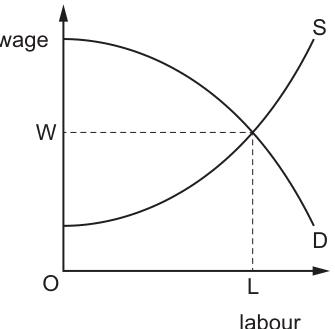
What is true about unit of labour L when they are paid wage W?
Options
A L is paid only economic rent.
B L is paid an element of economic rent and transfer earnings.
C L is paid below transfer earnings and leaves the industry.
D L is paid exactly transfer earnings and remains in work.
Reasoning
Transfer earnings are the minimum wage required to keep a unit of labour in its current employment, represented by the labour supply curve at each quantity of labour. Economic rent is any payment above this minimum. At the competitive labour market equilibrium, the wage W equals the marginal revenue product of labour, and for the marginal unit of labour L, the supply curve is exactly at wage W. This means the transfer earnings of L are equal to W, so L is paid exactly its transfer earnings and will remain in work.
Answer
D
D
Background Concept
In labour market analysis, transfer earnings refer to the minimum payment a worker requires to supply a unit of labour in a specific job. This is the worker's supply price for that unit of labour, and it is represented by every point on the labour supply curve: at any quantity of labour, the corresponding point on the supply curve shows the minimum wage needed to induce that worker to offer their labour. Economic rent is the excess payment a worker receives above their transfer earnings — it is the surplus over the minimum required to keep the worker in their current role. In a competitive labour market, the demand for labour equals the marginal revenue product of labour (MRP), as firms hire labour up to the point where the wage equals the additional revenue generated by the last worker.
Understanding the Question
The question provides a diagram of a competitive labour market, with equilibrium at wage W and employment level L (the intersection of the upward-sloping supply curve S and downward-sloping demand curve D). It asks which statement is true about the unit of labour L when paid the equilibrium wage W. The options test the distinction between transfer earnings and economic rent, and how these concepts apply to the marginal unit of labour at equilibrium. The task is to match the definitions of these terms to the features of the labelled diagram.
Approach
First, recall the formal definitions of transfer earnings and economic rent. Then, interpret the diagram: the supply curve S shows the transfer earnings of each unit of labour, while the horizontal dashed line at W is the actual wage paid to all employed workers. For the specific unit of labour L (the last worker hired at equilibrium), compare the wage W to the corresponding point on the supply curve to determine whether L is paid transfer earnings, economic rent, or both. Then evaluate each option against this comparison to identify the correct statement.
Step-by-Step Reasoning
- Define key terms clearly
- Transfer earnings: The minimum wage a worker will accept to supply a unit of labour in a given job. For any quantity of labour, the supply curve gives the transfer earnings of that unit.
- Economic rent: Any payment to a worker above their transfer earnings. It is the difference between the actual wage paid and the worker's supply price.
- Interpret the diagram's equilibrium
The labour market is competitive, so demand D equals the MRP of labour. The equilibrium is where D = S, at wage W and employment level L. All workers employed at this equilibrium are paid the same wage W. - Analyse the unit of labour L specifically
L is the marginal (last) unit of labour hired at the equilibrium wage. To find L's transfer earnings, look at the point on the supply curve S at quantity L: this point lies exactly on the horizontal line at wage W. This means L's transfer earnings are equal to W — W is the minimum wage this worker would accept to supply their labour.
Since the actual wage paid is exactly equal to L's transfer earnings, there is no economic rent paid to this unit of labour (economic rent would only exist if the wage was higher than the supply curve at L). - Evaluate each option
- Option A: Incorrect. L is not paid economic rent, as the wage equals its transfer earnings, so there is no excess payment above the minimum required.
- Option B: Incorrect. There is no economic rent component in L's pay, only transfer earnings.
- Option C: Incorrect. The wage W is equal to L's transfer earnings, not below it. If the wage was below transfer earnings, the worker would choose not to supply labour, but here the wage meets their minimum requirement.
- Option D: Correct. L is paid exactly its transfer earnings (W), so the worker is indifferent between staying in the job and leaving, but will remain in work as they receive their minimum required payment.
Key Takeaways
- The labour supply curve directly represents the transfer earnings of each unit of labour: every point on S is the minimum wage required for that unit of labour to be supplied.
- Economic rent is only paid to workers whose transfer earnings are below the equilibrium wage — these are workers employed at quantities below L, where the supply curve lies below W.
- The marginal unit of labour at the equilibrium quantity is always paid exactly its transfer earnings, with no economic rent.
- In a competitive labour market, the equilibrium wage is set by the intersection of labour demand (MRP) and labour supply, so all workers are paid the same wage regardless of their individual transfer earnings.
Common Mistakes
- Confusing transfer earnings and economic rent: Transfer earnings are the minimum required payment, while economic rent is the surplus above this minimum. Many students incorrectly assume all workers at the equilibrium wage earn economic rent, but this only applies to workers with transfer earnings below the equilibrium wage.
- Misinterpreting the supply curve: The supply curve shows the minimum wage for each unit of labour, not the actual wage paid. The actual wage is the horizontal line at W, set by the equilibrium.
- Focusing on the wrong unit of labour: The question asks specifically about unit L (the equilibrium quantity), not workers employed at lower quantities who do earn economic rent.
Things to Be Careful About
- Always link the supply curve to transfer earnings: each point on S is the transfer earnings of that specific unit of labour, so you must check the supply curve at the exact quantity L to find L's transfer earnings.
- For the marginal unit of labour at equilibrium, the wage will always equal the supply price (transfer earnings), so no economic rent is earned by this unit.
- Ensure you answer the exact question asked: the question refers only to unit L, so do not make claims about other units of labour employed at lower quantities.
What leads to an inflationary gap?
Options
A Aggregate demand is greater than the maximum potential output of the economy.
B Investment increases at a greater rate than profits received by a firm.
C The economy is operating below its full capacity.
D Innovation results in increased productivity in the economy.
Answer
An inflationary gap occurs when aggregate demand (AD) exceeds the economy's maximum potential output at full employment. This excess demand pulls up the general price level, creating demand-pull inflation.
Answer
A
A
Background Concept
An inflationary gap is a macroeconomic concept that describes a situation where the actual level of aggregate demand in an economy is greater than the economy's full-employment level of output (also called potential output). This gap is associated with demand-pull inflation. The opposite situation, where AD is less than potential output, is called a deflationary (or recessionary) gap, leading to unemployment and downward pressure on prices.
Understanding the Question
This is a multiple-choice question asking for the correct cause of an inflationary gap. The four options present different economic scenarios. The task is to select the one that accurately describes the condition that creates an inflationary gap.
Approach
Recall the definition of an inflationary gap: it is the amount by which actual aggregate demand exceeds the economy's potential output at full employment. Evaluate each option against this definition.
Step-by-Step Reasoning
- Option A: "Aggregate demand is greater than the maximum potential output of the economy." This is the textbook definition of an inflationary gap. When AD exceeds potential output, the economy is producing beyond its sustainable capacity, leading to upward pressure on prices (demand-pull inflation). This is correct.
- Option B: "Investment increases at a greater rate than profits received by a firm." This describes a firm-level financial situation, not a macroeconomic gap. It does not directly cause an inflationary gap.
- Option C: "The economy is operating below its full capacity." This describes a deflationary (recessionary) gap, not an inflationary gap. When the economy is below full capacity, there is a negative output gap, and inflation is typically low or negative.
- Option D: "Innovation results in increased productivity in the economy." Increased productivity shifts the long-run aggregate supply (LRAS) curve to the right, increasing potential output. This would tend to reduce an inflationary gap or create a deflationary gap, not cause one.
Therefore, only option A correctly identifies the cause of an inflationary gap.
Key Takeaways
- An inflationary gap is defined by AD exceeding potential output.
- It is associated with demand-pull inflation and a positive output gap.
- A deflationary gap is the opposite: AD is less than potential output.
- Understanding the difference between actual and potential output is crucial for analysing macroeconomic equilibrium.
Common Mistakes
- Confusing an inflationary gap with a deflationary gap (choosing option C).
- Thinking that any increase in investment (option B) automatically creates an inflationary gap, without considering the level of potential output.
- Assuming that productivity improvements (option D) cause inflation, when they actually increase supply and can be disinflationary.
Things to Be Careful About
- The question asks for what leads to an inflationary gap, not what happens during one. Option A describes the direct cause.
- Remember that an inflationary gap is a short-run phenomenon; in the long run, the economy may adjust through rising wages and prices, shifting the SRAS leftwards to restore equilibrium at potential output.
An open economy has a positive output gap.
What is likely to be decreasing?
Options
A expenditure on imports
B leisure time of workers
C nominal wage rates
D the general price level
Reasoning
A positive output gap means actual GDP exceeds potential GDP. The economy is operating above full employment, producing beyond its sustainable capacity. This is a boom phase of the business cycle.
In such conditions:
- Output and income are high, so expenditure on imports (A) would likely increase, not decrease.
- Workers are in high demand, often working overtime, so leisure time (B) would likely decrease.
- Strong demand for labour pushes nominal wage rates (C) up, not down.
- Strong aggregate demand puts upward pressure on the general price level (D), causing inflation, not deflation.
Therefore, the only variable likely to be decreasing is the leisure time of workers.
Answer
B
B
Background Concept
An output gap is the difference between the actual level of real GDP and the estimated potential level of real GDP (the maximum sustainable output an economy can produce without generating inflationary pressure).
- A positive output gap occurs when actual GDP > potential GDP. The economy is 'overheating' or in a boom. Resources, especially labour, are being used beyond their normal, sustainable capacity. Unemployment is below the natural rate.
- A negative output gap occurs when actual GDP < potential GDP. The economy is in a recession or slump with spare capacity and high unemployment.
The business cycle describes the fluctuations in actual GDP around the trend (potential) GDP, moving through phases of boom, recession, slump, and recovery.
Understanding the Question
The question states: "An open economy has a positive output gap." It then asks: "What is likely to be decreasing?"
You are given four options: expenditure on imports, leisure time of workers, nominal wage rates, and the general price level. The task is to identify which one of these is most likely to fall during a period when the economy is operating above its potential.
This is a multiple-choice question testing your understanding of the macroeconomic characteristics of a boom phase of the business cycle. The command word "What is likely to be decreasing?" requires you to apply your knowledge of the typical features of a positive output gap to each option and deduce the correct outcome.
Approach
- Recall the features of a positive output gap: High aggregate demand, high output, high employment (below natural rate), upward pressure on wages and prices, high levels of spending and investment.
- Analyse each option in turn: Consider the direction of change for each variable in the context of an overheating economy.
- Eliminate the options that would increase: Options A, C, and D are all variables that typically rise during a boom.
- Identify the option that would decrease: Option B is the only one that logically falls when the economy is running hot.
Step-by-Step Reasoning
Let's examine each option:
-
Option A: expenditure on imports. In an open economy with a positive output gap, domestic income and output are high. A rise in national income leads to a rise in the demand for imports (as imports are a positive function of income). Therefore, expenditure on imports is likely to be increasing, not decreasing. This option is incorrect.
-
Option B: leisure time of workers. A positive output gap means the economy is producing beyond its sustainable capacity. To achieve this, firms require more labour input. This can be achieved by hiring more workers (pushing unemployment below the natural rate) and by getting existing workers to work longer hours (overtime). As workers spend more time at work, their leisure time (time not spent in paid work or on personal obligations) necessarily decreases. This is the only option that is likely to be decreasing. This is the correct answer.
-
Option C: nominal wage rates. With the economy operating above full employment, the demand for labour is very high. There is a shortage of labour. To attract and retain workers, firms will bid up wages. Therefore, nominal wage rates are likely to be increasing, not decreasing. This option is incorrect.
-
Option D: the general price level. A positive output gap is characterised by demand-pull inflation. Aggregate demand exceeds the economy's ability to supply goods and services at stable prices. This excess demand pushes up the general price level. Therefore, the general price level is likely to be increasing (inflation), not decreasing. This option is incorrect.
Key Takeaways
- A positive output gap signifies an economy in a boom phase, operating above its potential.
- Key characteristics of a positive output gap include: high inflation, high employment (below natural rate), rising wages, high levels of spending and imports, and over-utilisation of resources (including labour).
- Understanding the relationship between the output gap and the labour market is crucial: a positive gap implies labour is being used intensively, reducing leisure time.
- This question tests the ability to apply macroeconomic theory to a specific scenario and deduce the logical consequence for different variables.
Common Mistakes
- Confusing a positive output gap with a negative one: A student might mistakenly think a positive output gap means the economy is doing well and workers have more leisure, or that prices are stable. It's important to remember that a positive gap means the economy is 'overheating'.
- Focusing on 'open economy' and overcomplicating the import option: While the 'open economy' detail is relevant for option A, it doesn't change the fundamental logic that higher income leads to higher imports. A student might incorrectly think about exchange rate effects, but the most direct and immediate effect is the income effect.
- Not considering the direction of change for all variables: A student might correctly identify that wages and prices rise but fail to consider the impact on leisure time. The question asks for what is decreasing, so it's essential to check each option against that specific criterion.
Things to Be Careful About
- Distinguish between actual and potential output: The output gap is the difference between these two. A positive gap means actual > potential.
- Understand the implications for the labour market: A positive output gap implies the economy is producing beyond its sustainable capacity, which requires more labour input than normal, reducing leisure.
- Remember the direction of change: The question asks for what is decreasing. Ensure you are not selecting an option that is increasing.
- Don't overthink: The most direct and logical answer is the one that follows from the basic definition of a positive output gap. The leisure time of workers is the only variable that clearly decreases in such a scenario.
In a two-sector economy, autonomous consumer expenditure increases by $100 billion, autonomous investment expenditure increases by $200 billion, and the marginal propensity to consume is 0.5.
What will the increase in National Income be?
Options
A $150 billion
B $300 billion
C $450 billion
D $600 billion
Working
Multiplier (k) = 1 / (1 - MPC) = 1 / (1 - 0.5) = 1 / 0.5 = 2
Total increase in autonomous expenditure = $100 billion + $200 billion = $300 billion
Increase in National Income = k x change in autonomous expenditure = 2 x $300 billion = $600 billion
Answer
D
D
Background Concept
In a two-sector economy (households and firms, no government and no foreign trade), the multiplier measures the number of times an initial change in autonomous expenditure (spending not dependent on income, such as autonomous consumption or investment) is multiplied to produce the final change in national income. The multiplier exists because one person's spending becomes another person's income, which is then partly spent again, creating a chain of additional rounds of spending. The size of the multiplier depends on the marginal propensity to consume (MPC) — the fraction of each additional dollar of income that is spent on consumption. The formula for the multiplier in a two-sector economy is:
k = 1 / (1 - MPC)
The change in national income is then:
Change in Y = k x Change in autonomous expenditure
Understanding the Question
This question gives us:
- An increase in autonomous consumer expenditure of $100 billion.
- An increase in autonomous investment expenditure of $200 billion.
- A marginal propensity to consume (MPC) of 0.5.
The economy is two-sector, so there is no government spending or taxation, and no imports or exports. The question asks for the total increase in National Income resulting from both injections together.
Approach
- Calculate the multiplier using the MPC.
- Add the two autonomous expenditure increases to find the total initial injection.
- Multiply the total injection by the multiplier to get the final change in National Income.
- Match the result to one of the four options.
Step-by-Step Reasoning
Step 1: Calculate the multiplier.
In a two-sector economy, the multiplier formula is:
k = 1 / (1 - MPC)
Given MPC = 0.5:
k = 1 / (1 - 0.5) = 1 / 0.5 = 2
This means that every $1 of autonomous spending will eventually generate $2 of national income.
Step 2: Find the total initial change in autonomous expenditure.
Both autonomous consumption and autonomous investment are injections into the circular flow. They are independent of income, so they add together:
Total injection = $100 billion + $200 billion = $300 billion
Step 3: Apply the multiplier.
Change in National Income = k x total injection = 2 x $300 billion = $600 billion
Step 4: Select the correct option.
Option D is $600 billion.
Key Takeaways
- The multiplier amplifies any change in autonomous expenditure.
- In a two-sector economy, the multiplier depends only on the MPC.
- Autonomous consumption and autonomous investment are both injections and their effects are additive.
- Always check the economy's structure (two-sector, three-sector with government, four-sector with foreign trade) because the multiplier formula changes when there are taxes or imports.
Common Mistakes
- Using only one injection: Some students might apply the multiplier to only the consumption increase or only the investment increase, forgetting that both are autonomous and both affect national income. This would give $200 billion or $400 billion, which are not even options, but the logic would be flawed.
- Incorrect multiplier formula: Using k = 1 / MPC (which would be 2 as well here, but is wrong in general) or k = MPC / (1 - MPC). The correct formula is k = 1 / (1 - MPC).
- Adding the MPC to the injection: Some might think the increase in income is simply the sum of the injections plus the MPC times something, which is not correct.
- Forgetting that the multiplier applies to the total injection: The multiplier applies to the sum of all autonomous changes, not to each separately and then added (though that would give the same result here, it is conceptually important to add first).
Things to Be Careful About
- The economy is two-sector, so there are no taxes or imports to reduce the multiplier. If the question had included a marginal tax rate or a marginal propensity to import, the formula would be different.
- The MPC is given as 0.5, so the multiplier is 2. A common trap is to think the multiplier is 1 / MPC = 2 as well, but that is a coincidence here; the correct formula is always 1 / (1 - MPC).
- The units are billions of dollars, so the answer is $600 billion, not 600.
- The question asks for the increase in National Income, not the new level of National Income. The answer is the change, not the final value.
Which government policy is least likely to promote inclusive economic growth?
Options
A increasing the national minimum wage
B investment in transport and infrastructure
C legislation reducing the power of trade unions
D using taxes and transfer payments to redistribute income
Answer
C. Legislation reducing the power of trade unions is the policy least likely to promote inclusive economic growth. Weakening trade unions typically reduces the bargaining power of lower-paid workers, potentially widening income inequality and limiting the extent to which the benefits of growth are shared. In contrast, the other three options directly target the incomes or opportunities of disadvantaged groups:
- A (increasing the national minimum wage) raises the floor for low-paid workers.
- B (investment in transport and infrastructure) improves access to employment and services.
- D (using taxes and transfer payments to redistribute income) directly narrows inequality.
C
Background Concept
Inclusive economic growth is growth whose benefits are widely shared across all segments of society, especially the poor and disadvantaged. It combines both an increase in national output (the 'growth' part) and a reduction in inequality of outcomes and opportunities (the 'inclusive' part). Policies that promote inclusive growth therefore must either directly raise the incomes of low-income groups (e.g. minimum wage, redistribution) or expand their access to productive resources and opportunities (e.g. infrastructure, education, labour rights).
Trade unions are organisations that bargain collectively on behalf of workers to improve wages, working conditions, and job security. Their power to do so depends on legal frameworks, union density, and the right to strike. Legislation that reduces union power weakens this bargaining function, typically lowering the wages of unionised workers (often lower- and middle-income) relative to what they would otherwise be. This can widen the gap between top earners and the rest, and reduce the share of national income going to labour compared to capital.
Understanding the Question
The question asks which of four government policies is least likely to promote inclusive economic growth. This is a comparative evaluation: each option must be assessed against the dual criterion of raising output and sharing its benefits more fairly. The command word is implicit in the multiple-choice format — the test-taker must reason through each option to identify the one that works against (or does least to advance) the goal of inclusive growth.
Option C stands out because weakening trade unions tends to worsen income distribution and reduce low-paid workers' share of growth, whereas the other three all have a direct positive impact on lower-income groups.
Approach
- Define inclusive economic growth.
- For each option, state the mechanism by which it might affect both growth and distribution.
- Identify which option works against (or does least for) distributional fairness, and explain why it is the 'least likely' to promote inclusive growth.
Step-by-Step Reasoning
-
Option A – increasing the national minimum wage
A higher minimum wage directly raises the earnings of the lowest-paid workers. Provided it is not set so high that it causes significant job losses, it reduces poverty and reduces inequality — both central to inclusivity. The growth effect is indirect (higher demand from low earners, possible productivity gains from reduced turnover), but the distributional effect is clearly positive. -
Option B – investment in transport and infrastructure
Better roads, public transport, and digital connectivity lower the cost of accessing jobs, education, and services, particularly for rural and low-income populations. This expands opportunities and raises potential output. The growth is inclusive because the new opportunities disproportionately benefit those who were previously excluded. -
Option D – using taxes and transfer payments to redistribute income
Progressive taxation combined with cash or in-kind transfers (e.g. child benefits, pensions, unemployment support) directly narrows post-tax income inequality. This targets the 'inclusive' dimension of growth most directly, even if its effect on the growth rate is more debatable (some argue it may dampen incentives; others argue it boosts aggregate demand). Overall, it is clearly supportive of inclusivity. -
Option C – legislation reducing the power of trade unions
Weakening unions reduces their ability to bargain for higher wages and better conditions. Unionised workers — many of whom are in lower- and middle-skill occupations — typically earn a premium over non-union workers. Removing or reducing that premium flattens or lowers the wage floor, widening the gap between top earners (whose earnings are set by market forces) and the rest. The gains from any resulting growth are less likely to flow to lower-income workers. This makes Option C the policy that is least likely to promote inclusive growth; indeed, it may actively work against it.
Key Takeaways
- Inclusive growth requires both an increase in output and a fair distribution of its benefits.
- Policies that weaken labour market institutions (such as trade unions) tend to increase inequality and therefore reduce inclusivity, even if they have some positive effect on output (e.g. by lowering labour costs for firms).
- Redistribution, minimum wage laws, and public investment are all broadly consistent with an inclusive growth agenda.
Common Mistakes
- Choosing Option A (minimum wage) because of the risk of unemployment — while a legitimate concern, the question asks which is least likely to promote inclusive growth, and minimum wage increase is generally considered a pro-inclusivity policy, especially at moderate levels.
- Choosing Option D because 'taxes reduce growth' — the question is about inclusive growth, not growth per se; redistribution directly improves inclusivity even if it slightly dampens the growth rate.
- Failing to consider the distributional dimension of each policy and focusing only on the growth dimension.
Things to Be Careful About
- The question is comparative: 'least likely' does not mean 'impossible' — the other three options are simply more clearly aligned with inclusive growth.
- 'Inclusive growth' is a specific concept; do not conflate it with 'economic growth' alone.
- Be ready to justify why weakening unions is more harmful to inclusivity than the potential costs of the other policies (e.g. unemployment from minimum wage, disincentive effects from redistribution).
What is an example of a demand-side macroeconomic policy that would reduce cyclical unemployment?
Options
A an increase in government spending on new infrastructure such as roads
B an increase in government spending on retraining workers
C a reduction in the rate of tax on imports
D an increase in the rate of tax on goods and services
Cyclical unemployment arises from a deficiency in aggregate demand (AD). A demand-side policy aims to increase AD. Option A, an increase in government spending on infrastructure, is an expansionary fiscal policy that directly increases AD, thereby reducing cyclical unemployment. Option B is a supply-side policy (improving labour mobility). Option C reduces the cost of imports, which may increase imports and worsen net exports, reducing AD. Option D increases taxes on goods and services, reducing consumption and AD, which would increase cyclical unemployment.
Answer
A
A
Background Concept
Cyclical unemployment (also called demand-deficient unemployment) occurs when there is insufficient aggregate demand in the economy to employ all those willing and able to work. It is associated with the downturn phase of the business cycle. Demand-side macroeconomic policies are those that influence the level of aggregate demand, primarily through fiscal policy (government spending and taxation) and monetary policy (interest rates and money supply). Supply-side policies, by contrast, aim to increase the productive capacity of the economy by improving labour markets, competition, or incentives.
Understanding the Question
The question asks for an example of a demand-side policy that would reduce cyclical unemployment. It presents four options, each describing a government action. The task is to identify which one is both demand-side and would reduce cyclical unemployment. The key is to recognise that cyclical unemployment is caused by low AD, so the correct policy must increase AD.
Approach
Evaluate each option in turn:
- Determine whether the policy is demand-side or supply-side.
- If demand-side, assess whether it increases or decreases AD.
- If it increases AD, it will reduce cyclical unemployment; if it decreases AD, it will worsen it.
- Only one option fits all criteria.
Step-by-Step Reasoning
Option A: Increase in government spending on new infrastructure such as roads.
Government spending is a component of AD (AD = C + I + G + (X-M)). An increase in G directly raises AD. This is an expansionary fiscal policy, a classic demand-side measure. Higher AD leads to higher output and employment, reducing cyclical unemployment. This is correct.
Option B: Increase in government spending on retraining workers.
Retraining improves the skills of workers, making them more employable in growing sectors. This addresses structural unemployment (mismatch of skills) rather than cyclical unemployment. It is a supply-side policy because it increases the quality and mobility of labour, shifting the long-run aggregate supply curve. It does not directly boost AD. Therefore, it is not a demand-side policy for cyclical unemployment.
Option C: Reduction in the rate of tax on imports.
A reduction in import taxes (tariffs) makes imports cheaper. This may increase the volume of imports. If imports rise, net exports (X-M) fall, reducing AD. This is a contractionary effect on AD, which would increase cyclical unemployment. Moreover, trade policy is not typically classified as a demand-side macroeconomic policy; it is more microeconomic or trade policy. So this is incorrect.
Option D: Increase in the rate of tax on goods and services.
An increase in indirect taxes (e.g., VAT) raises prices, reducing consumers' real purchasing power and thus consumption (C). Consumption is the largest component of AD, so AD falls. This is a contractionary fiscal policy, which would worsen cyclical unemployment. Hence incorrect.
Thus only Option A is a demand-side policy that reduces cyclical unemployment.
Key Takeaways
- Cyclical unemployment is caused by deficient aggregate demand.
- Demand-side policies aim to influence AD; the main ones are fiscal policy (government spending and taxation) and monetary policy.
- Supply-side policies target the productive capacity and labour market flexibility; they are not directly aimed at cyclical unemployment.
- When evaluating policies, always consider the direction of the effect on AD and the type of unemployment being addressed.
Common Mistakes
- Confusing supply-side policies (like retraining) with demand-side policies. Retraining is a supply-side measure to reduce structural unemployment, not cyclical.
- Thinking that any government spending is demand-side; but spending on retraining is supply-side because it improves labour supply, not AD.
- Misinterpreting tax changes: a reduction in import taxes may be seen as expansionary, but it actually reduces net exports, lowering AD.
- Failing to recognise that an increase in taxes on goods and services reduces consumption and AD, making cyclical unemployment worse.
Things to Be Careful About
- Always identify the type of unemployment first: cyclical, structural, frictional, etc.
- Distinguish between demand-side and supply-side policies clearly.
- Remember that government spending can be either demand-side (if it directly increases AD) or supply-side (if it improves productivity or labour supply). The purpose matters.
- In multiple-choice questions, eliminate obviously wrong options by applying economic reasoning step by step.
The diagram shows two liquidity preference curves LP1 and LP2.
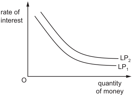
What would cause the liquidity preference curve to shift from LP1 to LP2?
Options
A There has been a fall in national income.
B There has been a rise in the general price level.
C There has been an increase in government borrowing.
D There has been an increase in the rate of interest.
Reasoning
The liquidity preference (LP) curve shows the quantity of money demanded at each rate of interest, ceteris paribus. A rightward shift from LP1 to LP2 means that at every interest rate, the public wishes to hold more money.
- Option A: A fall in national income reduces transactions demand for money, shifting the LP curve left, not right.
- Option C: Increased government borrowing raises the interest rate, causing a movement along the existing LP curve, not a shift.
- Option D: A rise in the interest rate is a change in the variable on the vertical axis, causing a movement along the LP curve, not a shift.
- Option B: A rise in the general price level increases the money needed for transactions, raising money demand at every interest rate and shifting the LP curve rightward from LP1 to LP2.
Answer
B
B
Background Concept
Keynesian liquidity preference theory explains the demand for money as the desire to hold liquid assets rather than interest-bearing assets like bonds. The demand for money has three motives: transactions demand (money needed for everyday purchases), precautionary demand (money held for unexpected expenses), and speculative demand (money held to take advantage of future changes in bond prices). The liquidity preference (LP) curve is a downward-sloping curve with the rate of interest on the vertical axis and the quantity of money demanded on the horizontal axis. It slopes downward because the interest rate is the opportunity cost of holding money: when interest rates are high, holding money means forgoing more interest income, so people hold less money; when interest rates are low, the opportunity cost is lower, so people hold more money.
Shifts in the LP curve are caused by changes in non-interest rate factors that affect the overall demand for money. These include changes in national income (higher income increases transactions demand, shifting LP right), changes in the general price level (higher prices increase the money needed for transactions, shifting LP right), and changes in expectations about future interest rates (if people expect interest rates to rise, they will hold more money now to buy bonds later when prices fall, increasing speculative demand and shifting LP right). Movements along the LP curve are caused only by changes in the interest rate itself, as this changes the quantity of money demanded via the opportunity cost effect.
Understanding the Question
The diagram shows the LP curve shifting rightward from LP1 to LP2. This means that at any given rate of interest, the quantity of money demanded has increased. The question asks which of the four options would cause this shift. To answer, we need to distinguish between factors that shift the LP curve (changes in non-interest rate determinants of money demand) and factors that cause a movement along the curve (changes in the interest rate, or changes that affect the interest rate rather than underlying money demand). We also need to identify which factor would increase money demand, leading to a rightward shift.
Approach
The core distinction to apply is between a shift in a curve and a movement along it:
- A shift in the LP curve is caused by a change in a factor other than the interest rate that affects the total demand for money.
- A movement along the LP curve is caused by a change in the interest rate itself, or a change that alters the interest rate without changing underlying money demand.
We will evaluate each option against this distinction, checking whether it increases money demand (rightward shift) or not.
Step-by-Step Reasoning
- First, confirm the meaning of the diagram: LP2 lies to the right of LP1, so at every interest rate, the quantity of money demanded is higher on LP2. This is a rightward shift of the LP curve, meaning total money demand has risen.
- Evaluate Option A: A fall in national income. National income is a key determinant of transactions demand for money: when income is higher, people spend more on goods and services, so they need to hold more money for transactions. A fall in income reduces spending, so transactions demand falls, shifting the LP curve to the left, not the right. Option A is incorrect.
- Evaluate Option C: An increase in government borrowing. When the government borrows more, it typically sells government bonds to the public to fund the deficit. This increases the demand for bonds, which pushes up the market interest rate (ceteris paribus). A change in the interest rate leads to a change in the quantity of money demanded, which is a movement along the existing LP curve (people hold less money as the interest rate rises, moving up along the curve). It does not shift the curve itself. Option C is incorrect.
- Evaluate Option D: An increase in the rate of interest. The interest rate is the variable on the vertical axis of the LP diagram. A change in the interest rate causes a change in the quantity of money demanded, which is a movement along the LP curve, not a shift. A higher interest rate would cause a movement up along the curve, reducing the quantity of money demanded, which is the opposite of the shift shown in the diagram. Option D is incorrect.
- Evaluate Option B: A rise in the general price level. The general price level determines how much money is required to purchase a given basket of goods and services. If prices rise, people need to hold more money to finance the same level of transactions, so the overall demand for money increases at every interest rate. This shifts the LP curve rightward, exactly as shown in the diagram. Option B is correct.
Key Takeaways
- The liquidity preference curve is the demand curve for money in Keynesian theory, downward sloping because the interest rate is the opportunity cost of holding money.
- Shifts in the LP curve are caused by changes in non-interest rate determinants of money demand: national income, the general price level, and expectations about future interest rates or bond prices.
- Movements along the LP curve are caused only by changes in the interest rate itself.
- A rightward shift of the LP curve means money demand has increased at every interest rate, which can be caused by higher national income, a higher price level, or expectations of lower future interest rates (which raise speculative demand for money).
Common Mistakes
- Confusing shifts and movements along the curve: A very common error is to select options that change the interest rate (such as increased government borrowing or a rise in the interest rate itself) as causes of a shift. These only cause a movement along the existing LP curve, not a shift.
- Misidentifying the effect of national income: Some students incorrectly think a fall in income increases money demand, but lower income means less spending and lower transactions demand, which shifts the LP curve left.
- Forgetting the link between the price level and transactions demand: Students may not connect a higher general price level to a higher need for money for daily purchases, so they fail to recognise that this is a valid shift factor.
Things to Be Careful About
- Always first identify whether a change affects the variable on the vertical axis (the interest rate) or a non-interest rate determinant of money demand: the former causes a movement along the curve, the latter causes a shift.
- Remember the direction of the effect of each determinant: higher national income or a higher price level increases money demand (shifts LP right), while lower income or lower prices decreases it (shifts LP left).
- Government borrowing affects the interest rate via increased demand for loanable funds, not the underlying demand for money, so it causes a movement along the LP curve, not a shift.
What does the Phillips curve show?
Options
A the relationship between economic growth and employment
B the relationship between inequality and income per capita
C the relationship between inflation and unemployment
D the relationship between prices and national income
Reasoning
The Phillips curve, named after A.W. Phillips, originally described an inverse relationship between the rate of wage inflation and the rate of unemployment. In modern macroeconomics, it is commonly interpreted as showing the relationship between general price inflation and unemployment. This is a core concept in the study of macroeconomic objectives and policy conflicts.
- Option A refers to the relationship between economic growth and employment, which is not what the Phillips curve shows (though there is a connection via Okun's law, but not the Phillips curve).
- Option B describes the Kuznets curve, not the Phillips curve.
- Option D relates to the aggregate demand and supply model or the quantity theory of money, not directly to the Phillips curve.
- Option C is the correct description: the Phillips curve shows the relationship between inflation and unemployment.
Answer
C
C
Background Concept
The Phillips curve is a fundamental concept in macroeconomics that illustrates the historical inverse relationship between the rate of inflation and the rate of unemployment. It was first observed by A.W. Phillips in 1958 for the UK economy. The original Phillips curve showed a trade-off: lower unemployment was associated with higher wage inflation. Later, it was adapted to show the relationship between price inflation and unemployment. The curve is central to understanding macroeconomic policy trade-offs, especially between the objectives of low inflation and low unemployment. The traditional Phillips curve suggests that policymakers face a choice: they can achieve lower unemployment only at the cost of higher inflation, and vice versa. However, the expectations-augmented Phillips curve (Friedman-Phelps) argues that in the long run, there is no trade-off; the long-run Phillips curve is vertical at the natural rate of unemployment. The short-run Phillips curve can shift due to changes in inflation expectations.
Understanding the Question
This is a straightforward multiple-choice question asking for the definition of the Phillips curve. The question tests basic knowledge of macroeconomic relationships. It expects the candidate to know which two variables the Phillips curve relates. The options are phrased to confuse the Phillips curve with other well-known economic relationships: the Kuznets curve (inequality and income per capita) and the aggregate demand-supply framework (prices and national income). The correct answer is the relationship between inflation and unemployment.
Approach
Recall the definition of the Phillips curve from your macroeconomic studies. Eliminate options that describe other economic models. The Phillips curve is specifically about inflation (or wage inflation) and unemployment. No calculation or deeper analysis is needed.
Step-by-Step Reasoning
- The Phillips curve is a graphical representation of the trade-off between inflation and unemployment.
- Option A: economic growth and employment – this relates to Okun's law (which links output and unemployment) or the business cycle, not the Phillips curve. Eliminate.
- Option B: inequality and income per capita – this is the Kuznets curve, not the Phillips curve. Eliminate.
- Option D: prices and national income – this is the aggregate demand and aggregate supply model (price level vs real GDP), not the Phillips curve. Eliminate.
- Option C: inflation and unemployment – this is exactly what the Phillips curve shows. Correct.
Key Takeaways
- The Phillips curve is a key policy tool illustrating the trade-off between inflation and unemployment in the short run.
- It is distinct from other curves like the Kuznets curve (income inequality) and the AD-AS model (price level vs output).
- Knowing the exact definitions of major economic curves is essential for multiple-choice questions.
Common Mistakes
- Confusing the Phillips curve with the Kuznets curve (inequality vs income).
- Thinking that the Phillips curve shows a relationship between economic growth and employment.
- Misremembering the axes: inflation (vertical) and unemployment (horizontal).
Things to Be Careful About
- The Phillips curve exists in both short-run and long-run versions, but the basic definition remains the same: inflation vs unemployment.
- The Phillips curve is not a demand or supply curve; it is a trade-off relationship.
- Make sure to distinguish between wage inflation and price inflation; the standard modern Phillips curve refers to price inflation.
A government is aiming to increase the role of market forces.
Which policy might achieve this?
Options
A deregulation
B nationalisation
C price controls
D production quotas
Reasoning
Market forces operate when supply and demand determine prices and quantities with minimal government intervention. Deregulation removes rules and restrictions, allowing market forces to play a larger role. The other options all increase government intervention: nationalisation transfers ownership from private to public sector; price controls override market prices; production quotas restrict the quantity supplied. Therefore, only deregulation increases the role of market forces.
Answer
A
A
Background Concept
Market forces refer to the natural interplay of supply and demand that determines prices, output, and resource allocation in a free market. Government intervention can reduce the role of these forces through regulations, state ownership, price controls, or quantity restrictions. Deregulation is a policy that removes or reduces government rules and restrictions, thereby allowing market forces to operate more freely. It is often considered a market-based supply-side policy intended to increase efficiency and competition.
Understanding the Question
The question asks which policy among the four options would help a government increase the role of market forces. The key is to understand whether each policy expands or contracts the scope of government intervention. The four options are:
- A: Deregulation
- B: Nationalisation
- C: Price controls
- D: Production quotas
Only one of these reduces government intervention and thus increases the role of market forces.
Approach
Evaluate each option in turn:
-
Deregulation: This involves removing or reducing government rules and regulations that constrain market activity. By eliminating barriers, firms can respond more freely to market signals, so market forces become stronger.
-
Nationalisation: This is the transfer of private assets to government ownership. The government then controls production and pricing decisions, often overriding market forces. This reduces the role of market forces.
-
Price controls: These are government-imposed limits on prices, such as price ceilings or floors. They prevent prices from adjusting to equilibrium, thus distorting market signals and reducing the role of supply and demand.
-
Production quotas: These are government-imposed limits on the quantity that can be produced or supplied. By restricting output, quotas override market forces and reduce the role of supply and demand.
Clearly, only deregulation aligns with the aim of increasing market forces.
Step-by-Step Reasoning
- Start with the definition: Market forces are the forces of supply and demand that determine equilibrium price and quantity without external interference.
- A government aiming to increase the role of market forces seeks to reduce its own intervention in the economy.
- Examine each option:
- Deregulation: Removing rules (e.g., licensing requirements, safety standards, or entry barriers) allows firms to compete more freely, and prices become more responsive to changes in supply and demand. This directly increases the role of market forces.
- Nationalisation: The government takes ownership of an industry. Decisions about what to produce, how much, and at what price are made by the state, not by market forces. This dramatically reduces the role of market forces.
- Price controls: Setting a maximum price (ceiling) or minimum price (floor) prevents the market from clearing at the equilibrium. For example, a rent control keeps prices below equilibrium, causing shortages and reducing the role of market forces. Similarly, a price floor above equilibrium causes surpluses.
- Production quotas: The government sets a limit on output. This restricts the quantity supplied, and the price is determined by demand at that quota, but the market cannot adjust to equilibrium. This reduces the role of market forces.
- Conclusion: Only deregulation increases the role of market forces; the other three policies increase government intervention and thus reduce market forces.
Key Takeaways
- Deregulation is a market-based policy that enhances the role of supply and demand.
- Nationalisation, price controls, and production quotas are interventionist policies that limit market forces.
- The question tests the basic understanding of the difference between policies that expand market freedom and those that restrict it.
Common Mistakes
- Confusing deregulation with nationalisation: Some students might think that nationalisation (taking control) can be used to increase market forces, but it actually does the opposite.
- Thinking that price controls are market-friendly because they are used in markets (e.g., agricultural price support) – but they override market prices.
- Believing that production quotas are just a way to manage supply without affecting market forces – but they are a direct restriction on quantity.
Things to Be Careful About
- The phrase “increase the role of market forces” is a clear signal that the policy should reduce government intervention.
- Read all options carefully; sometimes there can be subtle twists, but here the options are straightforward.
- Remember that deregulation is a supply-side policy that promotes competition and efficiency by removing barriers.
A country has a progressive income tax system.
What is not a valid reason for a government’s decision to reduce the rate of income tax paid on higher incomes?
Options
A to attract highly skilled workers from abroad
B to prevent tax evasion
C to provide work incentives
D to reduce income inequalities
Reasoning
A progressive income tax system takes a larger proportion of income from higher earners, reducing post-tax income inequality. Reducing the rate on higher incomes would increase the after-tax income of the wealthy relative to others, widening income inequality. Therefore, such a reduction cannot be a valid reason for a government aiming to reduce income inequalities.
The other options are valid reasons:
- A – Lower top tax rates can attract highly skilled workers from abroad, boosting the supply of labour and economic growth.
- B – Lower rates may reduce the incentive to engage in tax evasion, as the gain from evasion is smaller and compliance costs less.
- C – Lower marginal rates can provide work incentives for high earners, encouraging them to work more or invest more.
Answer
D
D
Background Concept
A progressive income tax system is one in which the average tax rate rises as income increases. This is typically used to achieve greater equity (fairness) by redistributing income from the rich to the poor. The trade-off between equity and efficiency is a central theme in public economics: policies that promote equity (e.g., high top tax rates) may reduce incentives to work, save, or invest, while policies that promote efficiency (e.g., low top tax rates) may worsen inequality. The question tests understanding of this trade-off by asking which of the listed reasons is inconsistent with the nature of a progressive tax.
Understanding the Question
The question presents a scenario: a country has a progressive income tax system. It then asks for the option that is NOT a valid reason for the government to reduce the rate of income tax paid on higher incomes. The command word is "What is not a valid reason?" – this is a negative multiple-choice question, meaning we must identify the option that does not logically follow from the stated policy goal (or that contradicts the goal of reducing inequality). Options A, B, and C are all plausible reasons that a government might offer to justify cutting top tax rates, often based on efficiency or administrative arguments. Option D, however, would be a reason to INCREASE top tax rates, not reduce them. The correct answer is therefore D.
Approach
To solve, evaluate each option against the likely effects of reducing the higher-income tax rate:
- A: Attracting highly skilled workers from abroad – a lower top rate makes the country more attractive to high-income earners, increasing the supply of talent. This is a supply-side argument and is often used to justify lower top rates.
- B: Preventing tax evasion – higher tax rates can increase the incentive to evade; lower rates may reduce evasion. This is a practical argument based on tax compliance.
- C: Providing work incentives – high marginal tax rates can reduce the incentive to work additional hours or take on more productive work; lower rates can increase effort and output. This is a standard efficiency argument.
- D: Reducing income inequalities – reducing the tax on higher incomes increases their post-tax income, widening the gap between rich and poor. This directly contradicts the goal of reducing inequality. Therefore, it is not a valid reason for reducing the rate.
Step-by-Step Reasoning
-
Identify the nature of the tax system: progressive means higher-income earners pay a higher percentage of their income in tax. This system is designed to reduce post-tax income inequality.
-
Analyze each option:
- Option A: If the government wants to attract highly skilled workers (e.g., engineers, doctors, executives) from other countries, a lower top tax rate increases the net reward for working in the country. This is a common policy in competitive global labour markets. So it is a valid reason.
- Option B: High tax rates can encourage tax evasion (e.g., hiding income, moving to tax havens). Lower rates reduce the benefit of evasion relative to the cost and risk, so compliance may improve. This is a valid reason.
- Option C: Income tax affects the reward for extra work. A high marginal rate reduces the take-home pay from additional work, which can discourage labour supply. Lowering the top rate can increase work incentives for high earners, boosting economic output. This is a valid reason.
- Option D: Reducing income inequalities is typically achieved by making the tax system more progressive, i.e., raising taxes on higher incomes, not lowering them. Cutting top rates increases post-tax income at the top, widening inequality. Thus, this reason is inconsistent with the policy change. It is NOT a valid reason.
-
Conclusion: The answer is D.
Key Takeaways
- Progressive taxation is a tool for redistribution; reducing top rates works against that goal.
- Governments often face a trade-off between equity (reducing inequality) and efficiency (growth, incentives).
- In multiple-choice questions, read the question carefully—especially negative ones like "not a valid reason".
- Understand the economic reasoning behind each policy option: each of A, B, C is a standard argument for lower top rates; D is the opposite.
Common Mistakes
- Choosing a valid reason because the question is phrased negatively. Always check which option is the exception.
- Confusing the direction of effect: thinking that lowering top rates could reduce inequality (it does the opposite).
- Overcomplicating: the question is straightforward once you recall that progressive tax reduces inequality, so cutting top rates cannot reduce inequality.
Things to Be Careful About
- The question asks for what is NOT a valid reason. Make sure you are selecting the one that does not fit.
- Do not assume that all reasons are about efficiency; D is about equity, and it contradicts the action.
- In a progressive system, reducing top rates is a regressive change, so it increases inequality.
A political party proposed a policy of quantitative easing (the creation of money by the central bank).
When would such a policy be least likely to destabilise the macroeconomy in the short run?
Options
A when the economy was experiencing a high level of inflation
B when the economy had price stability but there was full employment of the labour force
C when there was a deep recession with high levels of unemployment
D when there was full employment and a current account balance of payments deficit
Reasoning
Quantitative easing increases the money supply. In the short run, the effect on the macroeconomy depends on the state of aggregate supply. When the economy is in a deep recession with high unemployment, there is a large negative output gap. Aggregate supply is highly elastic, so an increase in aggregate demand from QE will mainly raise real output and employment rather than the price level. This is the least destabilising scenario because it avoids inflationary pressure. In contrast, when the economy is at full employment or experiencing high inflation, QE would primarily raise prices, destabilising the macroeconomy.
Answer
C
C
Background Concept
Quantitative easing (QE) is an unconventional monetary policy where a central bank creates new money electronically to purchase government bonds or other financial assets. This increases the money supply and aims to lower long-term interest rates, boost asset prices, and stimulate aggregate demand. The quantity theory of money (MV = PT) suggests that an increase in the money supply (M) will, if velocity (V) is stable, lead to a proportional increase in nominal output (PT). In the short run, this can be split into changes in real output (Y) and the price level (P), depending on the slope of the aggregate supply curve. When the economy has spare capacity (a negative output gap), the short-run aggregate supply curve is relatively flat, so an increase in AD raises real output more than prices. When the economy is at or near full capacity, the AS curve is steep, so the same increase in AD mainly raises prices.
Understanding the Question
The question asks: when would quantitative easing be least likely to destabilise the macroeconomy in the short run? 'Destabilise' here means causing high inflation or severe imbalances. We need to identify the scenario where QE is least inflationary and least likely to cause overheating. The four options describe different states of the economy: high inflation, price stability with full employment, deep recession with high unemployment, and full employment with a current account deficit. The correct answer is the one where the economy has the most spare capacity, so that the increase in money supply translates into output growth rather than inflation.
Approach
Evaluate each option based on the output gap and the slope of the short-run aggregate supply curve:
- Option A: High inflation suggests the economy is overheating, with a positive output gap. QE would add further demand pressure, worsening inflation and destabilising the economy.
- Option B: Price stability with full employment means the economy is at potential output. Any increase in AD from QE would push up prices, creating inflation and destabilising the economy.
- Option C: Deep recession with high unemployment implies a large negative output gap. The AS curve is flat, so QE can increase output without significant inflation. This is the least destabilising.
- Option D: Full employment with a current account deficit means the economy is at capacity. QE would increase AD, causing inflation and potentially worsening the current account deficit (as higher income boosts imports). This is destabilising.
Thus, C is the correct answer.
Step-by-Step Reasoning
- Quantitative easing increases the money supply. This is an expansionary monetary policy that shifts the aggregate demand curve to the right.
- The short-run effect on output and prices depends on the slope of the aggregate supply curve. The slope is determined by the amount of spare capacity in the economy.
- Option A: High level of inflation. This indicates that the economy is already operating above potential output (positive output gap). The AS curve is steep. An increase in AD will mainly raise the price level, worsening inflation. This is destabilising.
- Option B: Price stability but full employment. The economy is at potential output. The AS curve is vertical in the long run but may be upward-sloping in the short run. Any increase in AD will push up prices, creating inflation. This is destabilising.
- Option C: Deep recession with high unemployment. There is a large negative output gap. The AS curve is very flat (elastic). An increase in AD will mainly increase real output and employment, with little effect on the price level. This is the least destabilising scenario.
- Option D: Full employment and current account deficit. The economy is at capacity. QE will increase AD, causing demand-pull inflation. Additionally, higher income may increase imports, worsening the current account deficit. This is destabilising.
Therefore, the correct answer is C.
Key Takeaways
- The impact of monetary expansion on inflation depends critically on the state of the economy, specifically the output gap.
- In a recession with high unemployment, expansionary monetary policy can boost output without causing inflation (Keynesian range of AS).
- At full employment, the same policy is likely to be inflationary.
- Quantitative easing is not always inflationary; its effects are context-dependent.
Common Mistakes
- Assuming that an increase in the money supply always causes inflation. This ignores the possibility of spare capacity.
- Confusing the short run and long run. In the long run, money is neutral, but in the short run, it can affect real output.
- Not considering the slope of the aggregate supply curve.
- Overlooking the fact that QE is a form of monetary policy and its effects are similar to other expansionary monetary policies.
Things to Be Careful About
- The question specifies 'in the short run'. In the long run, the effects may differ (e.g., if expectations adjust).
- 'Destabilise' is interpreted as causing inflation or imbalances. In a recession, QE can stabilise the economy by boosting output, so it is least destabilising.
- Option D includes a current account deficit; while QE might worsen it, the primary destabilising effect is inflation. The current account deficit is a secondary concern.
- Always consider the output gap when evaluating the impact of demand-side policies.
What does the Laffer curve show?
Options
A the amount of tax revenue received at each tax rate
B the impact on the distribution of income after tax rates rise
C the rise in inflation following a fall in unemployment due to a cut in income tax
D the rise in poverty due to a rise in the basic rate of income tax
Answer
The Laffer curve shows the relationship between the tax rate and the total tax revenue received by the government. It suggests that as the tax rate rises from zero, revenue initially increases, but beyond a certain point further increases in the tax rate reduce revenue because they discourage economic activity.
Answer
A
A
Background Concept
The Laffer curve is a theoretical representation of the relationship between the rate of taxation and the resulting tax revenue. It is named after economist Arthur Laffer and is a key concept in supply-side economics. The curve is typically drawn as a bell-shaped or inverted-U curve. At a 0% tax rate, the government collects no revenue. As the tax rate increases, revenue rises because the government takes a larger share of each unit of income or profit. However, at very high tax rates, the disincentive effect becomes dominant: people work less, save less, invest less, or engage in tax avoidance and evasion, so the tax base shrinks. Eventually, the revenue starts to fall. The curve peaks at some tax rate (often argued to be around 30–50% in practice, though the exact point is disputed). The Laffer curve is used to argue that cutting tax rates can, under certain conditions, increase tax revenue by stimulating economic activity.
Understanding the Question
This is a straightforward multiple-choice question asking for the definition of the Laffer curve. The question provides four options, each describing a different possible relationship. The correct answer is the one that accurately captures what the curve shows: the amount of tax revenue received at each tax rate. The other options are plausible-sounding but incorrect: they refer to income distribution, the Phillips curve (inflation and unemployment), or poverty — none of which is what the Laffer curve directly illustrates.
Approach
Recall the definition of the Laffer curve. Compare each option against that definition. Option A is the textbook definition. Options B, C, and D are all related to other economic concepts (income distribution, the Phillips curve, and poverty) and are therefore incorrect.
Step-by-Step Reasoning
- The Laffer curve is a graph with the tax rate on the horizontal axis and tax revenue on the vertical axis.
- It shows that at a 0% tax rate, revenue is zero. As the tax rate rises, revenue increases, reaches a maximum, and then declines as the tax rate approaches 100%.
- Option A states: "the amount of tax revenue received at each tax rate." This is exactly what the curve shows.
- Option B: "the impact on the distribution of income after tax rates rise." The Laffer curve does not directly show income distribution; it shows total revenue. Income distribution is a separate issue (e.g., the Gini coefficient, Lorenz curve).
- Option C: "the rise in inflation following a fall in unemployment due to a cut in income tax." This describes the Phillips curve relationship, not the Laffer curve.
- Option D: "the rise in poverty due to a rise in the basic rate of income tax." The Laffer curve does not directly measure poverty; it measures revenue. While high tax rates might affect poverty indirectly, the curve itself does not show this.
Therefore, the correct answer is A.
Key Takeaways
- The Laffer curve is a supply-side concept showing the relationship between tax rates and tax revenue.
- It is used to argue that there is an optimal tax rate that maximises revenue, and that cutting taxes can sometimes increase revenue.
- Be careful not to confuse the Laffer curve with the Phillips curve (inflation and unemployment) or with distributional issues.
Common Mistakes
- Confusing the Laffer curve with the Phillips curve (option C). The Phillips curve shows the trade-off between inflation and unemployment, not tax revenue.
- Thinking the Laffer curve is about income distribution (option B) or poverty (option D). These are separate topics.
- Assuming that the Laffer curve always justifies tax cuts — it only shows a theoretical relationship; the actual shape and peak are debated.
Things to Be Careful About
- Read the options carefully. The Laffer curve is a specific diagram with a specific meaning.
- Remember that the Laffer curve is about tax revenue, not about the overall health of the economy or distributional equity.
- In an exam, if you are unsure, eliminate the clearly wrong options first (B, C, D) to arrive at A.
What are the variables identified on the axes of a Kuznets curve diagram?
Options
| vertical (Y) axis variable | horizontal (X) axis variable | |
|---|---|---|
| A | cumulative % of income | cumulative % of families |
| B | measure of inequality | income per capita |
| C | measure of standard of living | economic growth rate |
| D | income per capita | optimum population |
Reasoning
The Kuznets curve illustrates the hypothesis that inequality first increases and then decreases as an economy develops. Therefore the vertical axis measures inequality (e.g., the Gini coefficient) and the horizontal axis measures income per capita.
Answer
B
B
Background Concept
The Kuznets curve, named after economist Simon Kuznets, hypothesises that as an economy develops (measured by income per capita), market forces first increase and then decrease economic inequality. The curve is typically drawn with a measure of inequality (such as the Gini coefficient or the share of income held by the top x%) on the vertical axis and income per capita (or GDP per capita) on the horizontal axis. The shape is an inverted U: inequality rises during early industrialisation, then falls after a certain level of income is reached.
Understanding the Question
The question asks you to identify the correct pair of variables labelled on the axes of a Kuznets curve diagram. Four options are given, each pairing a vertical axis variable with a horizontal axis variable. You need to select the option that matches the standard Kuznets curve.
Approach
Recall the definition and purpose of the Kuznets curve. The curve is about the relationship between inequality and economic development. Therefore the vertical axis must be a measure of inequality, and the horizontal axis must be a measure of development (typically income per capita). Eliminate options that do not fit this pattern.
Step-by-Step Reasoning
- Option A: vertical = cumulative % of income, horizontal = cumulative % of families. This describes a Lorenz curve, not a Kuznets curve. The Lorenz curve plots cumulative income share against cumulative population share to show inequality at a single point in time. The Kuznets curve shows inequality over time or across income levels. So A is incorrect.
- Option B: vertical = measure of inequality, horizontal = income per capita. This exactly matches the standard Kuznets curve. The measure of inequality could be the Gini coefficient, the ratio of top to bottom income shares, etc. Income per capita is the standard proxy for economic development. So B is correct.
- Option C: vertical = measure of standard of living, horizontal = economic growth rate. The Kuznets curve does not use standard of living on the vertical axis; it uses inequality. Economic growth rate is a flow variable, not the stock variable typically used. So C is incorrect.
- Option D: vertical = income per capita, horizontal = optimum population. This reverses the axes and introduces the concept of optimum population, which is unrelated to the Kuznets curve. So D is incorrect.
Thus, only option B correctly identifies the variables.
Key Takeaways
- The Kuznets curve plots inequality (vertical) against income per capita (horizontal).
- Do not confuse it with the Lorenz curve, which plots cumulative income share against cumulative population share.
- The Kuznets curve is a hypothesis about the long-run relationship between development and inequality.
Common Mistakes
- Selecting option A because it involves inequality, but the Lorenz curve is a different diagram. The question specifically asks for the Kuznets curve.
- Confusing the axes: some might think inequality is on the horizontal axis or that income per capita is on the vertical axis.
- Not knowing the standard definition of the Kuznets curve.
Things to Be Careful About
- Remember that the Kuznets curve is about inequality and development, not about living standards or growth rates.
- The horizontal axis is typically income per capita (a measure of development), not economic growth rate (which is a percentage change).
- The vertical axis is a measure of inequality, not a cumulative share (which is for the Lorenz curve).
What might cause income inequality to worsen in a country?
Options
A increased discrimination
B increased labour market participation
C increased skill level of workers
D increased welfare payments
Increased discrimination restricts the income-earning opportunities of certain groups, widening the gap between high and low earners. The other options either reduce inequality (increased welfare payments, increased labour market participation that brings low-income groups into work) or have ambiguous effects (increased skill levels may raise low-income productivity).
Answer
A
A
Background Concept
Income inequality refers to the extent to which income is distributed unevenly among a population. It is typically measured using the Gini coefficient or the Lorenz curve. Factors that can worsen inequality include those that concentrate income among a small group, such as discrimination, unequal access to education, and regressive government policies. Discrimination in the labour market reduces the earnings of certain groups (e.g., based on gender, race, or ethnicity), lowering their relative income and increasing overall inequality.
Understanding the Question
The question asks which of the four options is a cause of worsening income inequality. You are given four possible factors: increased discrimination, increased labour market participation, increased skill level of workers, and increased welfare payments. The task is to identify which one would unambiguously increase the gap between rich and poor. The answer is increased discrimination, as it is a barrier to equal opportunity and earnings.
Approach
Evaluate each option in turn, considering whether it tends to increase or decrease income inequality. For discrimination, the effect is clear: it reduces the incomes of the discriminated group. For the other options, consider their typical effects: increased labour market participation can raise the incomes of previously excluded groups, reducing inequality; increased skill levels can raise the wages of low-skilled workers if they receive training, reducing inequality; increased welfare payments are redistributive and directly reduce inequality. Therefore, only discrimination worsens inequality.
Step-by-Step Reasoning
-
Option A: Increased discrimination. Discrimination in hiring, pay, or promotion reduces the earnings of certain groups. This lowers their relative income, widening the gap between them and the non-discriminated majority. Thus, inequality worsens.
-
Option B: Increased labour market participation. If more people enter the workforce, especially from low-income groups, their earnings increase, which can reduce the income gap. While participation might be concentrated in low-wage jobs, it still raises their income relative to zero, so overall inequality tends to fall (or at least not worsen). Therefore, this is not a cause of worsening inequality.
-
Option C: Increased skill level of workers. If the skill level of low-income workers rises, their productivity and wages increase, reducing inequality. If the skill level of high-income workers rises, the effect could be ambiguous, but the question says 'skill level of workers' generally, which typically implies an overall improvement in human capital, which tends to reduce inequality by raising the earnings of the lower-skilled. Thus, not a cause of worsening.
-
Option D: Increased welfare payments. Welfare payments are transfers to the poor, directly increasing their income and reducing inequality. This is a redistributive policy that improves equity. So it does not worsen inequality.
Therefore, only A is correct.
Key Takeaways
- Discrimination is a market failure that creates inequality by preventing equal access to income.
- Policies that increase labour market participation, skill levels, or welfare payments typically reduce inequality, not worsen it.
- In multiple-choice questions, test each option against the concept of 'worsening inequality'.
Common Mistakes
- Confusing 'increased labour market participation' with 'increased inequality' – if participation increases among low-income groups, inequality falls.
- Thinking that increased skill levels always benefit the already-skilled – in reality, skill improvements can raise the incomes of the low-skilled.
- Overlooking the redistributive nature of welfare payments.
Things to Be Careful About
- Read each option carefully and consider the direction of the effect on income distribution.
- Remember that inequality is about the gap, not just the level of income. A factor that raises everyone's income equally does not change inequality; discrimination lowers the income of some, widening the gap.
- The question is about 'cause' – not 'what might reduce inequality' – so focus on factors that increase the gap.
A multinational company is planning to invest in a new factory in a low-income country.
What is not a possible benefit to the low-income country?
Options
A acquiring improved technology
B better training for the workforce
C extra tax revenue for the government
D increased competition for small domestic producers
Answer
Options A, B, and C are all potential benefits of inward foreign direct investment by a multinational company: the host country gains access to advanced technology, improved human capital through training, and additional tax revenue. Option D, increased competition for small domestic producers, is a potential cost or disadvantage, not a benefit. Hence, D is the correct answer.
D
Background Concept
Multinational companies (MNCs) are firms that operate in multiple countries. When an MNC invests in a new factory in a low-income country, this is a form of foreign direct investment (FDI). FDI can bring several benefits to the host country, including technology transfer, workforce training, infrastructure development, and increased tax revenue. However, it can also have negative effects, such as crowding out local businesses, environmental damage, and exploitation of labour. The question asks which of the listed options is NOT a possible benefit, meaning it is either neutral or a drawback.
Understanding the Question
The question presents four possible outcomes of an MNC building a factory in a low-income country. The task is to identify which one is not a benefit. Three of the options are widely recognised as potential gains for the host economy, while one is typically seen as a cost or risk. The correct answer is the option that represents a disadvantage rather than an advantage.
Approach
Evaluate each option in turn:
- A: Acquiring improved technology – is this a benefit? Yes, technology transfer can boost productivity and long-term growth.
- B: Better training for the workforce – is this a benefit? Yes, it enhances human capital and employability.
- C: Extra tax revenue for the government – is this a benefit? Yes, it increases public funds for infrastructure and services.
- D: Increased competition for small domestic producers – is this a benefit? Typically, increased competition can be a benefit for consumers (lower prices, more choice), but for small domestic producers it is a threat that may force them out of business. From the perspective of the low-income country as a whole, the net effect of competition is ambiguous; however, the question specifically asks about a benefit to the country. Increased competition for small domestic producers is generally considered a potential cost (loss of local businesses, jobs, and income) rather than a benefit. Therefore, D is not a possible benefit.
Step-by-Step Reasoning
- Option A: MNCs often bring advanced machinery, production techniques, and know-how that are not available locally. This can improve productivity and efficiency in the host economy, leading to higher output and growth. This is a clear benefit.
- Option B: MNCs typically train local workers to operate new equipment and meet quality standards. This raises the skill level of the workforce, which can increase wages and employability, and may spill over to other sectors. This is a benefit.
- Option C: The MNC will pay taxes (corporate income tax, property tax, etc.) to the host government. This additional revenue can be used for public goods and services, such as education, healthcare, and infrastructure. This is a benefit.
- Option D: The new factory will compete with existing small domestic producers. This competition may drive them out of business if they cannot match the MNC's lower costs or superior products. While consumers may benefit from lower prices, the question asks about a benefit to the low-income country. The loss of local businesses can reduce local employment, income, and entrepreneurial activity, and may increase economic dependence on the MNC. Therefore, increased competition for small domestic producers is generally considered a potential cost, not a benefit. Hence, D is the correct answer.
Key Takeaways
- FDI by MNCs can bring technology, training, and tax revenue, which are benefits for the host country.
- Increased competition for local firms is a double-edged sword: it can benefit consumers but harm domestic producers. In the context of a low-income country with vulnerable small businesses, it is often viewed as a cost.
- When a question asks for what is NOT a benefit, look for the option that represents a disadvantage or a neutral effect.
Common Mistakes
- Choosing D because one thinks competition is always good. While competition can improve efficiency, the question specifically asks about a benefit to the low-income country, and the impact on small domestic producers is typically negative. Some students might incorrectly see competition as a benefit overall, but the phrasing "increased competition for small domestic producers" highlights the harm to local firms, making it a cost.
- Misreading the question: forgetting the word "not" and selecting a benefit instead.
- Assuming that all options are benefits because MNCs are often portrayed positively.
Things to Be Careful About
- Read the question carefully: "What is not a possible benefit?" means you need to identify the option that is not a benefit.
- Understand the perspective: the benefit is to the low-income country as a whole, not just to consumers or the MNC.
- Recognise that "increased competition for small domestic producers" is a cost to those producers, and while it may have some positive effects (e.g., lower prices for consumers), the net effect on the country's development can be negative, especially if small businesses are a major source of employment and income. The question lists it as a separate option, and it is clearly not a straightforward benefit like the others.
- In multiple-choice questions, eliminate the three that are clearly benefits; the remaining one is the answer.
A country with fixed exchange rates faces a surplus on its current account.
Which policy is most desirable to maintain the fixed exchange rate?
Options
A an increase in subsidies given to exporters
B the imposition of trade barriers on the import of non-essential goods
C the sale of foreign currencies in the foreign exchange market
D the use of expansionary monetary policy
Reasoning
A current account surplus means export revenue exceeds import spending. Foreign buyers of exports need the domestic currency to pay for them, so demand for the domestic currency rises. Under a fixed exchange rate, the central bank must prevent the currency from appreciating. It does this by selling the domestic currency (or buying foreign currency) in the foreign exchange market, increasing the supply of the domestic currency to meet the excess demand. Option C describes the sale of foreign currencies, which is the opposite of what is needed — the central bank would buy foreign currency (selling domestic currency) to maintain the peg. Option D, expansionary monetary policy, lowers domestic interest rates, which reduces the capital account surplus and also reduces demand for the domestic currency, easing the upward pressure. However, the most direct and immediate policy to maintain the fixed rate in the face of a current account surplus is for the central bank to sell domestic currency and buy foreign currency. Option C is the closest description of this intervention, but it states the sale of foreign currencies, which is the reverse. Option D is the most desirable among the given choices because it addresses the underlying cause by reducing the interest rate differential that attracts capital inflows, thereby reducing demand for the domestic currency.
Answer
D
D
Background Concept
Under a fixed exchange rate system, the central bank commits to keeping the value of its currency within a narrow band against another currency or a basket of currencies. To do this, it must intervene in the foreign exchange market whenever market forces push the exchange rate away from the target. A current account surplus means the country is exporting more than it is importing. Foreign buyers of exports must obtain the domestic currency to pay for them, which increases demand for the domestic currency in the foreign exchange market. This excess demand would normally cause the domestic currency to appreciate. To prevent this appreciation and maintain the fixed rate, the central bank must increase the supply of the domestic currency in the market. It does this by selling the domestic currency and buying foreign currency (using its foreign exchange reserves). This intervention adds to the supply of the domestic currency, offsetting the excess demand and keeping the exchange rate at the target level.
Understanding the Question
The question presents a scenario: a country with a fixed exchange rate is running a current account surplus. It asks which policy is "most desirable" to maintain the fixed exchange rate. The four options are different policy actions. The key is to identify which action directly addresses the upward pressure on the domestic currency caused by the surplus. The question tests understanding of the mechanics of foreign exchange intervention and the relationship between the current account and the exchange rate.
Approach
First, establish the effect of a current account surplus on the foreign exchange market: it creates excess demand for the domestic currency. To maintain the fixed rate, the central bank must counteract this excess demand. The most direct method is to sell the domestic currency (or buy foreign currency) in the market. Evaluate each option against this requirement:
- Option A: Subsidies to exporters would increase exports further, worsening the surplus and increasing demand for the domestic currency. This is counterproductive.
- Option B: Trade barriers on imports would reduce imports, increasing the surplus further. This is also counterproductive.
- Option C: The sale of foreign currencies means the central bank is selling foreign currency and buying domestic currency. This would reduce the supply of domestic currency, increasing its value further. This is the opposite of what is needed.
- Option D: Expansionary monetary policy (lowering interest rates) reduces the capital account surplus by making domestic assets less attractive to foreign investors. This reduces demand for the domestic currency, easing the upward pressure. While not a direct intervention in the foreign exchange market, it addresses the underlying cause and is the most desirable among the given options.
Step-by-Step Reasoning
- Identify the problem: A current account surplus means exports > imports. Foreign buyers need the domestic currency to pay for exports, so demand for the domestic currency increases.
- Effect on exchange rate: Under a floating rate, the domestic currency would appreciate. Under a fixed rate, the central bank must prevent this appreciation.
- Required intervention: To prevent appreciation, the central bank must increase the supply of the domestic currency or reduce demand for it. The direct method is to sell domestic currency (buy foreign currency) in the foreign exchange market.
- Evaluate Option A: Subsidies to exporters would make exports cheaper, increasing export volume and the surplus. This would increase demand for the domestic currency, making the problem worse. Not desirable.
- Evaluate Option B: Trade barriers on imports would reduce imports, increasing the surplus further. This would also increase demand for the domestic currency. Not desirable.
- Evaluate Option C: Selling foreign currencies means the central bank is buying domestic currency with foreign currency. This reduces the supply of domestic currency in the market, which would cause it to appreciate. This is the opposite of the required intervention. Not desirable.
- Evaluate Option D: Expansionary monetary policy (e.g., lowering interest rates) makes domestic assets less attractive to foreign investors. This reduces capital inflows, which reduces demand for the domestic currency. It also may stimulate domestic spending, increasing imports and reducing the current account surplus. Both effects reduce the upward pressure on the exchange rate. This is the most desirable option among the four.
Key Takeaways
- A current account surplus creates excess demand for the domestic currency in the foreign exchange market.
- To maintain a fixed exchange rate, the central bank must counteract this by selling the domestic currency (buying foreign currency).
- Monetary policy can also be used to influence the exchange rate by affecting capital flows and the current account.
- The question tests the ability to link a balance of payments component to the foreign exchange market and to evaluate policy options.
Common Mistakes
- Choosing Option C because it mentions "sale of foreign currencies" which sounds like intervention. The mistake is not realising that selling foreign currency means buying domestic currency, which would cause appreciation.
- Thinking that subsidies or trade barriers would help by boosting exports or reducing imports, without considering that these actions would worsen the surplus and increase demand for the domestic currency.
- Not understanding that the central bank's intervention to prevent appreciation involves selling the domestic currency, not buying it.
Things to Be Careful About
- Read the direction of the intervention carefully: "sale of foreign currencies" means the central bank is selling foreign currency and buying domestic currency. This is the opposite of what is needed to prevent appreciation.
- Remember that a current account surplus puts upward pressure on the exchange rate, not downward pressure.
- Consider both direct intervention (foreign exchange market operations) and indirect policies (monetary policy) that can affect the exchange rate.
Which criticism of foreign direct investment (FDI) is least valid?
Options
A It encourages competition, reduces prices and forces the less efficient domestic firms to leave the market.
B It brings workers from its own country and provides only low paying jobs to low skilled local workers.
C It is usually withdrawn quickly in case of a global crisis, making developing countries more vulnerable to global shocks.
D Its actions often result in environmental degradation, and over exploitation of natural resources.
Reasoning
FDI typically brings capital, technology, and managerial expertise into a host economy. It often increases competition, which can lower prices and force inefficient domestic firms out of the market. This is a valid criticism from the perspective of domestic firms that cannot compete, but it is a benefit for consumers and the economy overall. The question asks for the least valid criticism — the one that is not a genuine drawback of FDI.
Option A describes a situation where FDI encourages competition, reduces prices, and forces less efficient domestic firms to leave. This is actually a positive outcome of FDI (increased efficiency and lower consumer prices), not a valid criticism. The other options (B, C, D) describe genuine negative consequences: low-quality jobs, capital flight during crises, and environmental damage.
Answer
A
A
Background Concept
Foreign Direct Investment (FDI) occurs when a firm from one country invests directly in production or business facilities in another country, typically by establishing subsidiaries or acquiring local firms. FDI is a key channel through which multinational corporations (MNCs) operate. It brings capital, technology, management skills, and access to international markets to the host economy. While FDI has many potential benefits (economic growth, job creation, technology transfer, increased competition), it also attracts several criticisms, particularly in developing countries.
Understanding the Question
This question asks which of the four statements is the least valid criticism of FDI. The key word is "criticism" — we are looking for a statement that is supposed to be a negative aspect of FDI. The "least valid" criticism is the one that is either not a genuine negative consequence, or is actually a positive outcome mischaracterised as a negative one. We need to evaluate each option against economic theory and real-world evidence.
Approach
Examine each option in turn:
- Determine whether it describes a genuine negative consequence of FDI.
- If it describes a positive outcome, it is not a valid criticism.
- The option that is least valid is the one that is either factually incorrect or misrepresents a benefit as a drawback.
Step-by-Step Reasoning
Option A: "It encourages competition, reduces prices and forces the less efficient domestic firms to leave the market."
- This describes increased competition leading to lower prices and the exit of inefficient firms. From the perspective of consumers and the overall economy, this is a benefit of FDI — it improves allocative efficiency and consumer welfare. The only party harmed is the inefficient domestic firms themselves, but the question asks for a criticism of FDI in general, not a criticism from the viewpoint of a specific group. Therefore, this is not a valid criticism of FDI; it is a positive outcome. This makes it the least valid criticism.
Option B: "It brings workers from its own country and provides only low paying jobs to low skilled local workers."
- This is a genuine criticism. MNCs may bring expatriate workers for higher-skilled positions, while local workers are offered low-skilled, low-wage jobs with limited opportunities for advancement. This can exacerbate inequality and limit the developmental impact of FDI.
Option C: "It is usually withdrawn quickly in case of a global crisis, making developing countries more vulnerable to global shocks."
- This is a valid criticism. FDI can be volatile — during a global financial crisis or economic downturn, MNCs may repatriate capital, close operations, or reduce investment, leaving host countries exposed to sudden stops and capital flight. This increases the vulnerability of developing economies to external shocks.
Option D: "Its actions often result in environmental degradation, and over exploitation of natural resources."
- This is a well-documented criticism. MNCs may operate with lower environmental standards in developing countries, leading to pollution, deforestation, resource depletion, and other environmental harms. This is a genuine negative consequence of FDI.
Since Option A describes a benefit rather than a drawback, it is the least valid criticism.
Key Takeaways
- FDI has both positive and negative effects on host economies.
- Increased competition and lower prices are generally considered benefits, not criticisms.
- Valid criticisms of FDI include: low-quality jobs, capital flight during crises, environmental degradation, exploitation of natural resources, and limited technology transfer.
- When evaluating statements, distinguish between genuine negative consequences and outcomes that are positive for the economy as a whole.
Common Mistakes
- Misreading the question: the question asks for the least valid criticism, not the most valid one. Some students might pick the most obviously negative statement instead.
- Confusing a benefit with a criticism: Option A is a positive outcome for consumers and the economy, but a student might see "forces less efficient domestic firms to leave" and think it is a criticism, without recognising that this is a normal competitive process that improves efficiency.
- Not considering the perspective: the question asks for a criticism of FDI in general, not from the viewpoint of a specific stakeholder (e.g., domestic firms).
Things to Be Careful About
- Read the question carefully: "least valid" means the statement that is the weakest or most incorrect as a criticism.
- Understand that increased competition and lower prices are generally seen as benefits of FDI, not drawbacks.
- Recognise that the other three options (B, C, D) are all genuine and commonly cited criticisms of FDI in developing countries.
Your score so far
Answer a question to start scoring
Your marks add up here as you work through the paper.