Economics 9708/33 — October/November 2025
Cambridge A-Level · A Level Multiple Choice · answer key with instant marking and worked solutions
Topics Government Policies to Correct Market Failure · Costs of Production · Effectiveness of Macroeconomic Policies · Macroeconomic Objectives and Policy Conflicts · Economic Development and Living Standards · Economic Growth and Sustainability · +13 more
Tap an option under each question to check it — your score builds as you go.
Why would an economy wish to achieve economic efficiency?
Options
A to achieve an equal distribution of income
B to achieve full employment
C to ensure resources are not wasted
D to ensure international competitiveness
Answer
Economic efficiency means that resources are allocated in a way that maximises the total benefit to society from their use. Achieving this ensures that resources are not wasted — that is, no reallocation could make someone better off without making someone else worse off (Pareto optimality).
C
Background Concept
Economic efficiency is a central concept in microeconomics. It has two main components:
- Productive efficiency: producing goods and services at the lowest possible cost (on the production possibility frontier).
- Allocative efficiency: producing the mix of goods and services that consumers most value (where price equals marginal cost).
When an economy achieves both, it is using its scarce resources to maximise total welfare. The opposite — inefficiency — means resources are being wasted: either too much of some goods and too little of others, or goods are being produced at unnecessarily high cost.
Understanding the Question
This is a multiple-choice question asking for the fundamental reason an economy would want to achieve economic efficiency. The options present four possible goals: equal income distribution, full employment, avoiding waste, and international competitiveness. The question tests whether you understand that efficiency is about getting the most out of limited resources — not about equity, employment, or trade performance.
Approach
Read each option and ask: "Is this the primary purpose of economic efficiency, or is it a separate goal that may or may not be helped by efficiency?"
- A (equal distribution) is about equity, not efficiency. Efficiency can coexist with inequality.
- B (full employment) is a macroeconomic objective; efficiency is about how resources are used, not whether they are all used.
- C (avoid waste) is the direct definition of efficiency.
- D (international competitiveness) is a possible outcome of efficiency but not its core purpose.
Step-by-Step Reasoning
- Recall the definition of economic efficiency: it means that resources are allocated to their highest-valued uses, so that no reallocation could increase total welfare. This is equivalent to saying that no resources are wasted.
- Option A: An equal distribution of income is a normative goal about fairness. An efficient allocation can be very unequal (e.g., a market outcome where the rich get most goods). Efficiency does not guarantee equity.
- Option B: Full employment means all willing workers have jobs. But even at full employment, resources could be misallocated — producing the wrong goods or using outdated technology. Efficiency is about how they are used, not whether they are used.
- Option C: This is the essence of efficiency. If resources are wasted, society could be better off by reallocating them. Avoiding waste is the direct reason for pursuing efficiency.
- Option D: International competitiveness is a possible benefit of efficiency (lower costs, better products), but it is not the fundamental reason. An economy could be efficient and still not be competitive if other countries are even more efficient.
Therefore, the correct answer is C.
Key Takeaways
- Economic efficiency is about maximising welfare from scarce resources — avoiding waste.
- It is distinct from equity (fairness), full employment, and competitiveness.
- In multiple-choice questions, always match the option to the precise definition, not to a related but different concept.
Common Mistakes
- Choosing A (equal distribution) because efficiency sounds like a good thing and fairness is also good. But they are separate goals.
- Choosing B (full employment) because efficiency is often discussed alongside employment. But efficiency is about allocation, not the level of employment.
- Choosing D (international competitiveness) because efficient firms are often competitive. But the question asks why an economy would wish to achieve efficiency — the reason is to avoid waste, not to beat other countries.
Things to Be Careful About
- Read the question carefully: it asks for the reason an economy would wish to achieve efficiency, not a possible consequence.
- Distinguish between the definition of a concept and its potential benefits. The definition is the core reason.
A firm has set a low price in the short run to act as a barrier to entry for new firms entering the market.
This is an example of which pricing strategy?
Options
A limit pricing
B predatory pricing
C price discrimination
D price leadership
Answer
The firm is setting a low price specifically to deter new firms from entering the market. This is the defining purpose of limit pricing: a price set low enough to make entry unattractive for potential competitors, while still allowing the existing firm to earn at least normal profit. Predatory pricing, by contrast, involves temporarily setting a price below cost to drive existing rivals out of the market, not to block entry. Price discrimination charges different prices to different customers for the same good, and price leadership occurs when one firm sets a price that others follow. The correct answer is therefore A.
Answer
A
A
Background Concept
Firms in imperfectly competitive markets (especially oligopolies and monopolies) can use pricing strategies to influence market structure and their own profitability. Three key strategies are often confused:
-
Limit pricing: Setting a price low enough that potential entrants would find it unprofitable to enter the market. The existing firm sacrifices some short-run profit to maintain its long-run market power. The price is typically set just below the entry-inducing price level, so that a new firm entering would face a price below its average cost and make a loss.
-
Predatory pricing: Temporarily setting a price below cost (or very low) with the intention of driving existing competitors out of the market. Once they exit, the predator raises prices again to recoup losses. This is illegal in many jurisdictions.
-
Price discrimination: Charging different prices to different consumers for the same product, based on differences in their willingness to pay, not on differences in cost.
-
Price leadership: An informal arrangement in an oligopoly where one firm (usually the largest or most efficient) sets a price, and other firms follow suit to avoid price wars.
Understanding the Question
The question presents a specific scenario: "A firm has set a low price in the short run to act as a barrier to entry for new firms entering the market." The key phrase is "to act as a barrier to entry" — the purpose is to prevent new firms from entering, not to drive out existing ones. The question asks which pricing strategy this describes.
Approach
- Identify the purpose of the low price: to block entry.
- Match this purpose to the definition of each pricing strategy.
- Eliminate strategies whose purpose does not match.
Step-by-Step Reasoning
-
Option A: Limit pricing — The textbook definition of limit pricing is exactly this: a price set low enough to deter entry. The firm accepts lower short-run profit to protect its long-run market position. This matches the scenario perfectly.
-
Option B: Predatory pricing — Predatory pricing targets existing competitors, not potential entrants. Its goal is to drive them out, after which the predator raises prices. The question says "to act as a barrier to entry for new firms," not to eliminate current rivals. So B is incorrect.
-
Option C: Price discrimination — This strategy is about charging different prices to different customers, not about setting a low price to block entry. It has nothing to do with barriers to entry. So C is incorrect.
-
Option D: Price leadership — This is a coordination mechanism in oligopoly, where one firm's price change is followed by others. It does not involve setting a low price to deter entry. So D is incorrect.
Therefore, the only option that matches the scenario is A.
Key Takeaways
- The key distinction between limit pricing and predatory pricing is the target: limit pricing targets potential entrants (to block entry), while predatory pricing targets existing rivals (to drive them out).
- Both involve low prices, but their purposes and time horizons differ.
- Understanding the precise definition of each pricing strategy is essential for multiple-choice questions.
Common Mistakes
- Confusing limit pricing with predatory pricing because both involve low prices. The critical difference is whether the low price is aimed at blocking entry (limit pricing) or driving out existing competitors (predatory pricing).
- Thinking that any low price set by a dominant firm must be predatory. The question explicitly states the purpose is to act as a barrier to entry, which is the hallmark of limit pricing.
Things to Be Careful About
- Read the scenario carefully: the phrase "to act as a barrier to entry" is the decisive clue.
- Do not overthink: the question tests a straightforward definition, not a complex analysis.
- Remember that limit pricing is a long-term strategy (sacrificing short-run profit for long-run market power), while predatory pricing is a short-term tactic followed by a price increase.
A dentist is found to have charged patients for treatment they did not need.
What is the likely cause of this market failure?
Options
A a minimum price
B asymmetric information
C non-excludability
D productive inefficiency
Working
The dentist has superior knowledge about the necessity of treatment compared to the patient. This is a classic case of asymmetric information, where one party (the dentist) has more information than the other (the patient). This leads to market failure because the patient cannot make an informed decision, resulting in an inefficient outcome (over-treatment).
Answer
B
B
Background Concept
Asymmetric information occurs when one party in a transaction has more or better information than the other. In markets, this imbalance can lead to market failure because the less-informed party cannot make optimal decisions, resulting in an inefficient allocation of resources. Common examples include the market for 'lemons' (used cars), insurance markets (moral hazard), and professional services (doctors, dentists, mechanics).
Understanding the Question
The question describes a dentist charging patients for unnecessary treatment. The dentist knows whether the treatment is needed; the patient does not. This is a clear case of asymmetric information. The question asks for the likely cause of market failure, so we must identify which of the four options best explains why this situation leads to inefficiency.
Approach
We need to recall the standard causes of market failure: externalities, public goods, asymmetric information, and market power. Then match the scenario to the correct cause. The dentist's exploitation of superior knowledge fits asymmetric information. The other options can be eliminated: a minimum price is a policy, not a cause; non-excludability is a feature of public goods; productive inefficiency is a consequence, not a cause.
Step-by-Step Reasoning
- Identify the key feature: the dentist knows more than the patient about the necessity of treatment.
- This is asymmetric information: the seller (dentist) has information advantage over the buyer (patient).
- Asymmetric information leads to market failure because the patient cannot make a fully informed choice, so resources are misallocated (unnecessary treatment is provided).
- Evaluate other options:
- A minimum price: This is a government intervention, not a cause of market failure. It could be a response to market failure, but not the cause here.
- Non-excludability: This is a characteristic of public goods, where it is impossible to exclude non-payers. Dental services are excludable (patients can be refused treatment if they don't pay).
- Productive inefficiency: This means producing at a cost higher than the minimum. The dentist may be inefficient, but the core problem is the information asymmetry that allows overcharging, not inefficiency in production.
- Therefore, the correct answer is B: asymmetric information.
Key Takeaways
- Asymmetric information is a common cause of market failure in markets where one party has more information than the other.
- It can lead to adverse selection (before transaction) and moral hazard (after transaction).
- In professional services, information asymmetry often results in over-treatment or overcharging.
- Recognising real-world examples helps in applying economic concepts.
Common Mistakes
- Confusing asymmetric information with externalities: externalities involve third-party effects, not information imbalance.
- Thinking that any market failure is due to externalities: many market failures have other causes.
- Selecting 'productive inefficiency' because the dentist is not producing efficiently: but the question asks for the cause, not a consequence.
- Overlooking the information advantage: the dentist's knowledge is the key.
Things to Be Careful About
- Read the scenario carefully: the dentist is charging for unnecessary treatment, which directly points to information asymmetry.
- Distinguish between causes of market failure and policies to correct them: a minimum price is a policy, not a cause.
- Remember the definitions: non-excludability is about public goods, not relevant here.
- In multiple-choice questions, eliminate clearly wrong options first to narrow down.
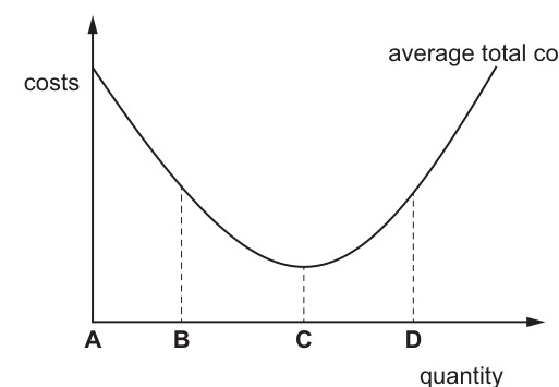
The diagram shows the average total cost for a firm.
At what level of output does marginal cost exceed average total cost?
Options
A output level A on Fig. 4.1
B output level B on Fig. 4.1
C output level C on Fig. 4.1
D output level D on Fig. 4.1
Working
Marginal cost (MC) intersects average total cost (ATC) at the minimum point of the ATC curve. At output C, MC equals ATC. To the right of C, ATC is rising, which occurs only when MC exceeds ATC. Output D lies to the right of the minimum point.
Answer
D
D
Background Concept
In microeconomics, the marginal-average relationship explains how marginal and average values interact. For cost curves specifically, the marginal cost (MC) curve intersects the average total cost (ATC) curve at its minimum point. When MC is below ATC, each additional unit costs less than the current average, pulling the average down and causing ATC to fall. When MC exceeds ATC, each additional unit costs more than the current average, pulling the average up and causing ATC to rise. Only when MC equals ATC is the average stationary at its minimum (or maximum) point.
Understanding the Question
The question presents a U-shaped average total cost curve with four output levels marked: A, B, C, and D. Point C is identified as the minimum point of the ATC curve. The question asks at which output level marginal cost exceeds average total cost. This requires applying the marginal-average relationship to determine the region where ATC is rising, which corresponds to the portion of the curve to the right of its minimum.
Approach
Since MC intersects ATC at its minimum point (output C), MC equals ATC at C. To the left of C (outputs A and B), ATC is downward sloping, meaning MC must be below ATC. To the right of C (output D), ATC is upward sloping, meaning MC must be above ATC. Therefore, the output level where MC exceeds ATC is D.
Step-by-Step Reasoning
- The diagram displays the average total cost (ATC) curve, which is U-shaped, reflecting initially falling and then rising average costs as output increases.
- Point C corresponds to the minimum point of the ATC curve.
- Economic theory establishes that the marginal cost (MC) curve intersects the ATC curve precisely at its minimum point. Thus, at output level C, MC = ATC.
- For output levels between A and C, the ATC curve is falling (downward sloping). This can only occur if MC < ATC, because the cost of producing an additional unit is below the current average, dragging the average down.
- For output levels to the right of C, such as D, the ATC curve is rising (upward sloping). This can only occur if MC > ATC, because the cost of producing an additional unit is above the current average, pushing the average up.
- Therefore, at output level D, marginal cost exceeds average total cost.
Key Takeaways
The marginal-average relationship is a fundamental principle that applies to costs, revenue, and productivity. When a marginal value lies below an average value, the average falls; when the marginal value lies above the average, the average rises; and when they are equal, the average is at its extremum. For U-shaped cost curves, MC always intersects both ATC and AVC at their respective minimum points. Recognizing whether an average curve is rising or falling is the key to determining the position of the marginal curve relative to it.
Common Mistakes
- Selecting output C: This is incorrect because C represents the minimum point where MC equals ATC, not exceeds it.
- Selecting outputs A or B: These are incorrect because at these outputs ATC is falling, indicating that MC is below ATC.
- Confusing absolute cost levels with the marginal-average relationship: The question depends on whether ATC is rising or falling, not on whether costs are high or low in absolute terms.
Things to Be Careful About
The question specifically asks where marginal cost exceeds average total cost. This is a strict inequality (MC > ATC). The minimum point C represents equality (MC = ATC) and therefore does not satisfy the condition. Only the region where ATC is rising satisfies MC > ATC. Always check the slope of the average curve at the point in question: if it is rising, marginal exceeds average; if falling, marginal is below average.
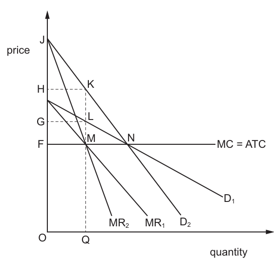
The diagram shows the effect of a demand curve shift from D1 to D2 for a profit maximising firm.
What has happened to the firm’s total revenue and the deadweight welfare loss?
Options
| total revenue | deadweight welfare loss | |
|---|---|---|
| A | decreases to OGLQ | decreases by KLN |
| B | decreases to OGLQ | increases by KLN |
| C | increases to OHKQ | decreases by KLN |
| D | increases to OHKQ | increases by KLN |
Reasoning
The firm is a profit-maximising monopoly, facing downward-sloping demand (D) and marginal revenue (MR) curves, with constant marginal cost (MC = ATC, shown as a horizontal line).
- The demand curve shifts rightward from D1 to D2, representing an increase in demand. The new marginal revenue curve (MR2) lies to the right of the original MR1, so the profit-maximising output (where MR = MC) rises. The price is set from the new demand curve D2 at this higher output, and is higher than the original price.
- Total revenue (TR) is calculated as price multiplied by quantity (P × Q). With both price and quantity higher than the original equilibrium, TR increases to the rectangular area OHKQ.
- Deadweight welfare loss (DWL) is the loss of total surplus caused by the monopoly producing below the socially optimal output level (where demand = MC, the allocatively efficient outcome). When demand increases, the socially optimal output rises, and the gap between the monopoly's restricted output and the socially optimal output widens, while the demand curve is higher. This makes the DWL triangle larger. The increase in DWL is the area KLN, the difference between the new and original DWL.
Answer
D
D
Background Concept
A monopoly is a market structure with a single firm, which is a price maker facing a downward-sloping market demand curve. The firm's marginal revenue (MR) curve lies below its demand curve, as it must lower price for all units to sell more output. Profit maximisation occurs where marginal revenue equals marginal cost (MR = MC). Constant marginal cost (MC = ATC, horizontal) means each additional unit costs the same to produce, and average total cost is equal to marginal cost at all output levels.
Total revenue (TR) is the total income a firm earns from sales, calculated as price (P) multiplied by quantity sold (Q), represented graphically as the rectangular area under the price up to the quantity sold.
Allocative efficiency occurs where the price consumers are willing to pay equals the marginal cost of production (D = MC), meaning resources are allocated to their most valued uses. A monopoly restricts output below this allocatively efficient level to raise price and profit, creating a deadweight welfare loss (DWL): the lost total surplus (consumer surplus + producer surplus) that would exist if the market were perfectly competitive. The DWL is represented by the triangle between the demand curve, the MC curve, and the vertical line at the monopoly's output level.
Understanding the Question
The question provides a diagram of a monopoly with constant MC, and shows a rightward shift in the demand curve from D1 to D2 (an increase in demand). It asks what happens to the firm's total revenue and the size of the deadweight welfare loss as a result of this shift. This is a 1-mark multiple-choice question requiring you to apply your knowledge of monopoly pricing, revenue calculation, and deadweight loss to the given diagram.
Approach
To solve this, follow these steps:
- Identify the original and new profit-maximising equilibria using the MR = MC rule.
- Calculate original and new total revenue as P × Q, using the price from the demand curve at each equilibrium quantity.
- Identify the original and new deadweight welfare loss triangles, then compare their sizes to find the change.
- Match your findings to the options provided.
Step-by-Step Reasoning
-
Original equilibrium (D1): The original marginal revenue curve MR1 intersects the horizontal MC curve at point M, corresponding to quantity Q. The price is set from the original demand curve D1 at quantity Q, which is H (point K on D1). Original total revenue is TR1 = H × Q, represented by the rectangular area OHKQ (from the origin O up to price H on the vertical axis, across to quantity Q on the horizontal axis, and down to the origin).
-
New equilibrium (D2): The rightward shift in demand to D2 raises the marginal revenue curve to MR2, which intersects MC at a higher quantity than Q. The new price is set from D2 at this higher quantity, which is higher than H. New total revenue is TR2 = new P × new Q, which is larger than TR1, so TR increases to the rectangular area OHKQ (the area corresponding to the new higher price and higher quantity).
-
Original deadweight welfare loss: The socially optimal output level (where D = MC, allocative efficiency) for the original demand D1 is the quantity where D1 intersects MC (point N). The original DWL is the triangle between D1, MC, and the vertical line at the original monopoly quantity Q: this is the area of lost total surplus because the monopoly produces Q instead of the socially optimal quantity. The area of this triangle is proportional to the gap between the monopoly price and MC, and the gap between the socially optimal quantity and the monopoly quantity.
-
New deadweight welfare loss: After demand shifts right to D2, the socially optimal output level is higher (where D2 intersects MC, which is a higher quantity than the original socially optimal level). The new DWL is the larger triangle between D2, MC, and the vertical line at the new higher monopoly quantity. The increase in DWL is the area KLN: this is the additional lost surplus caused by the larger gap between the monopoly's restricted output and the new higher socially optimal output, plus the higher value of the lost units due to the higher demand.
-
Matching to the options: Total revenue increases to OHKQ, and DWL increases by KLN, which corresponds to option D.
Key Takeaways
- For a monopoly, total revenue is always the rectangular area under the price up to the profit-maximising quantity (P × Q), not the area under the demand curve.
- A rightward shift in demand (increase in demand) for a monopoly raises both total revenue (as long as the output effect does not outweigh the price effect negatively, which is typical for a demand increase) and deadweight welfare loss, because the underproduction relative to the allocatively efficient level becomes more severe.
- Deadweight welfare loss from monopoly is always the triangle between the demand curve, the MC curve, and the vertical line at the monopoly's output level.
Common Mistakes
- Reversing the demand shift direction: Assuming a shift from D1 to D2 is a decrease in demand, leading to the wrong conclusion about TR and DWL changes. Always check which curve is the new one: a rightward shift is an increase, leftward is a decrease.
- Miscalculating total revenue: Confusing TR with consumer surplus or producer surplus. TR is always the rectangle P × Q, not a triangle.
- Misidentifying the DWL area: The DWL is the triangle between demand and MC, not between MR and MC, and not the area of profit.
- Assuming DWL always falls when output rises: Even if the monopoly increases output after a demand rise, the socially optimal output rises by more, so the DWL increases.
Things to Be Careful About
- Always use the MR = MC rule to find the profit-maximising quantity, not the demand curve.
- Use the demand curve (not MR) to find the profit-maximising price, as the demand curve shows the maximum price consumers will pay for that quantity.
- When calculating the change in DWL, compare the area of the original DWL triangle to the new one: the difference is the change, which in this case is the area KLN.
- Ensure you match the direction of the demand shift correctly: the question states the shift is from D1 to D2, so D2 is the new demand curve.
A firm sells 10 000 units per month at a price of $10. The firm’s total fixed cost is $40 000 per month. The firm makes only normal profit.
What is the average variable cost for this output?
Options
A $2.00
B $4.00
C $6.00
D $8.00
Working
Total revenue (TR) = Price × Quantity = $10 × 10 000 = $100 000.
Normal profit means total revenue equals total cost (TR = TC).
Therefore, total cost (TC) = $100 000.
Total fixed cost (TFC) = $40 000.
Total variable cost (TVC) = TC − TFC = $100 000 − $40 000 = $60 000.
Average variable cost (AVC) = TVC / Quantity = $60 000 / 10 000 = $6.00.
Answer
C
C
Background Concept
This question tests the relationship between revenue, costs, and profit, specifically the condition for normal profit.
- Total Revenue (TR) is the total income a firm receives from selling its output: TR = Price × Quantity.
- Total Cost (TC) is the sum of all costs of production. It is split into Total Fixed Cost (TFC), which does not vary with output (e.g., rent), and Total Variable Cost (TVC), which does vary with output (e.g., raw materials).
- Profit is TR − TC.
- Normal profit is the minimum level of profit needed to keep a firm in its current line of production. It is considered a cost of production (the opportunity cost of the entrepreneur's resources). In economic terms, when a firm makes only normal profit, its total revenue exactly equals its total cost (TR = TC). This means the firm is covering all its explicit and implicit costs, including the opportunity cost of capital and entrepreneurship, but is making no supernormal profit (economic profit above normal).
Understanding the Question
The question gives us:
- Quantity sold per month: 10 000 units.
- Price per unit: $10.
- Total Fixed Cost per month: $40 000.
- The firm makes only normal profit.
We are asked to find the Average Variable Cost (AVC) for this output. AVC is calculated as TVC / Quantity. We know TFC and Quantity, so we need to find TVC. The key to finding TVC is using the normal profit condition to first find TC.
Approach
- Calculate Total Revenue (TR) from the given price and quantity.
- Apply the normal profit condition: TR = TC. This gives us Total Cost (TC).
- Calculate Total Variable Cost (TVC) using the formula: TVC = TC − TFC.
- Calculate Average Variable Cost (AVC) using the formula: AVC = TVC / Quantity.
- Match the result to one of the options.
Step-by-Step Reasoning
-
Calculate Total Revenue (TR):
TR = Price × Quantity = $10 × 10 000 = $100 000. -
Apply the Normal Profit Condition:
The question states the firm makes "only normal profit." In economics, this means the firm's total revenue is exactly equal to its total cost. There is no supernormal profit. Therefore:
TR = TC
$100 000 = TC
So, Total Cost (TC) = $100 000. -
Calculate Total Variable Cost (TVC):
We know that Total Cost (TC) is the sum of Total Fixed Cost (TFC) and Total Variable Cost (TVC).
TC = TFC + TVC
We can rearrange this to find TVC:
TVC = TC − TFC
TVC = $100 000 − $40 000 = $60 000. -
Calculate Average Variable Cost (AVC):
AVC is the variable cost per unit of output.
AVC = TVC / Quantity
AVC = $60 000 / 10 000 = $6.00. -
Select the Correct Option:
The calculated AVC is $6.00, which corresponds to option C.
Key Takeaways
- Normal profit is a crucial concept. It is not the same as zero profit in an accounting sense. It means the firm is covering all its costs, including opportunity costs, and earning just enough to stay in business. The condition TR = TC is the defining characteristic of normal profit.
- Understanding the breakdown of Total Cost into Fixed and Variable components is fundamental to cost analysis.
- This question demonstrates a common exam technique: using a given condition (like normal profit) to find a missing piece of information (TC) and then using that to calculate another variable (AVC).
Common Mistakes
- Confusing normal profit with zero accounting profit: A student might think normal profit means the firm is making no money and incorrectly set TR = 0 or Profit = 0, leading to a wrong calculation of TC.
- Forgetting the definition of normal profit: A student might try to calculate profit as a separate unknown, rather than using the condition TR = TC.
- Miscalculating AVC: A student might correctly find TVC but then divide by the wrong number or forget to divide at all, e.g., stating AVC = $60 000.
- Confusing AVC with AFC or ATC: A student might calculate Average Fixed Cost (AFC = TFC/Q = $4.00) and mistakenly select option B, or calculate Average Total Cost (ATC = TC/Q = $10.00) and not find it in the options.
Things to Be Careful About
- Read the condition carefully: The phrase "only normal profit" is the single most important piece of information. It is the key that unlocks the whole calculation.
- Keep track of units: The costs are given in dollars per month, and quantity is in units per month. The final answer is in dollars per unit ($6.00).
- Work step-by-step: Write down each step clearly. This helps avoid arithmetic errors and makes it easy to check your work.
- Check your answer against the options: After calculating $6.00, verify that it is one of the choices. If it isn't, you know you made a mistake somewhere in your reasoning.
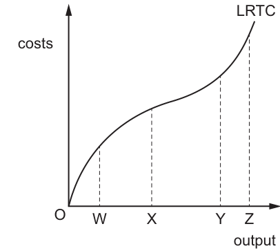
The diagram shows the long-run total cost (LRTC) curve of a firm.
At which output is the long-run average total cost at its minimum?
Options
A OW
B OX
C OY
D OZ
Answer
Long-run average total cost (LRAC) equals LRTC divided by output (LRAC = LRTC / Q). The minimum LRAC occurs where a straight line from the origin O is tangent to the LRTC curve, as at this point the slope of LRTC equals LRAC. In the given diagram, this tangency is at output OY, so the correct option is C.
C
Background Concept
Long-run total cost (LRTC) is the total cost incurred by a firm when producing a given level of output in the long run, when all factors of production are variable and the firm can adjust its plant size to the optimal level for any output. Long-run average total cost (LRAC) is the cost per unit of output in the long run, calculated as LRTC divided by the quantity of output produced: LRAC = LRTC / Q.
The shape of the LRAC curve is determined by economies and diseconomies of scale. When a firm experiences economies of scale as output increases (for example, bulk purchasing discounts, specialisation of labour, or more efficient use of large machinery), LRAC falls. When it experiences constant returns to scale, LRAC remains constant at its lowest level. When diseconomies of scale set in (for example, coordination problems in large firms, higher managerial costs), LRAC rises. The lowest point on the LRAC curve is called the minimum efficient scale (MES): the smallest output level at which a firm can produce at the lowest possible long-run average cost.
The LRTC curve is typically S-shaped. It first increases at a decreasing rate (reflecting increasing returns to scale, where LRAC is falling), then may have a section where it increases at a constant rate (constant returns to scale, flat LRAC), and finally increases at an increasing rate (reflecting decreasing returns to scale, where LRAC is rising). The inflection point of the LRTC curve (where the curve changes from increasing at a decreasing rate to increasing at an increasing rate) is not the same as the minimum LRAC point.
Understanding the Question
The question provides a diagram of a firm's LRTC curve, with four output levels marked on the horizontal axis: OW, OX, OY and OZ. It asks which of these output levels corresponds to the minimum long-run average total cost. This is a 1-mark multiple choice question that tests the candidate's understanding of the mathematical relationship between LRTC and LRAC, and their ability to apply this relationship to interpret a cost curve diagram.
Approach
To solve this question, we use the mathematical relationship between LRTC and LRAC, and a standard graphical rule to identify the minimum LRAC point from the LRTC curve:
- Recall that LRAC = LRTC / Q. To find the minimum of this function, we look for the point where the slope of the LRTC curve equals the LRAC value.
- Graphically, this minimum point is found where a straight line drawn from the origin (O) to a point on the LRTC curve is tangent to the curve. This is because the slope of the ray from the origin to the point (LRTC/Q) is exactly the LRAC value, and tangency means the slope of the LRTC curve at that point equals the slope of the ray.
- We apply this rule to the given diagram to check which output level (OW, OX, OY, OZ) matches this tangency point.
Step-by-Step Reasoning
- First, analyse each output option against the tangency rule:
- Output OW: The ray from the origin to the point on the LRTC curve at OW is steeper than the LRTC curve at that point. This means LRAC (the slope of the ray) is higher than the slope of LRTC, so LRAC is still falling as output rises beyond OW. OW cannot be the minimum.
- Output OX: This is the inflection point of the LRTC curve, where the curve changes from increasing at a decreasing rate to increasing at an increasing rate. The ray from the origin to the point on LRTC at OX is still less steep than the LRTC curve for outputs between OX and OY, meaning LRAC continues to fall as output rises from OX to OY. OX is not the minimum.
- Output OY: The ray from the origin to the point on the LRTC curve at OY is exactly tangent to the LRTC curve. At this point, the slope of LRTC equals the LRAC value, so this is the minimum point of the LRAC curve.
- Output OZ: The ray from the origin to the point on the LRTC curve at OZ is less steep than the LRTC curve at that point. This means LRAC is now higher than the slope of LRTC, so LRAC is rising as output rises beyond OY. OZ is not the minimum.
- The only output that satisfies the tangency condition is OY, so the correct answer is option C.
Key Takeaways
- The fundamental relationship between long-run total cost and long-run average cost is LRAC = LRTC / Q.
- The minimum point of the LRAC curve (minimum efficient scale) can be identified graphically as the point where a ray from the origin is tangent to the LRTC curve.
- The inflection point of the LRTC curve is not the minimum LRAC point: the inflection point is where the slope of LRTC is smallest, while the minimum LRAC is where the slope of LRTC equals the average cost.
Common Mistakes
- Confusing the inflection point with the minimum LRAC: A common error is to select OX, which is the inflection point of the LRTC curve. Candidates often incorrectly assume that the point where the LRTC curve changes its rate of increase is the minimum LRAC, but this is not the case. The inflection point only marks where the slope of LRTC stops decreasing and starts increasing, not where LRAC is lowest.
- Selecting the point where LRTC rises most steeply: Some candidates may choose OZ, the output where LRTC is rising at the fastest rate, but this is where LRAC is already rising, not at its minimum.
- Forgetting the tangency rule: Without recalling the origin-tangency condition, candidates may guess randomly or select an option based on an incorrect assumption about the shape of the curves, leading to wrong answers.
Things to Be Careful About
- Always apply the origin-tangency rule when identifying the minimum LRAC from an LRTC diagram, rather than relying on visual cues like the inflection point or the steepest part of the curve.
- Verify that the selected output corresponds to the point where the ray from the origin is exactly tangent to the LRTC curve, not just a point on the curve.
- Remember that the minimum LRAC is the minimum efficient scale, the lowest possible cost per unit the firm can achieve in the long run when all factors are variable.
Assuming there are no externalities, where would a nationalised firm set output to maximise social welfare?
Options
A where average revenue equals average cost
B where average revenue equals marginal cost
C where marginal revenue equals marginal cost
D where marginal revenue is zero
Answer
In the absence of externalities, social welfare is maximised when price equals marginal cost. For a nationalised firm, price is given by average revenue (AR). Therefore, the firm should set output where AR = MC. This is option B.
B
Background Concept
Social welfare in economics is typically measured by the sum of consumer surplus and producer surplus. Under perfect competition and no externalities, the market outcome where price equals marginal cost (P = MC) achieves allocative efficiency and maximises total surplus. A nationalised (state-owned) firm is often instructed to pursue social welfare rather than private profit. Its demand curve is the same as the market demand curve, so average revenue (AR) equals price. Therefore, the condition for social welfare maximisation is AR = MC.
Understanding the Question
The question asks where a nationalised firm should set output to maximise social welfare, assuming no externalities. The options present four different output rules. The key is to recognise that a nationalised firm's objective differs from a private profit-maximising firm. The correct rule is the one that achieves allocative efficiency.
Approach
Recall the condition for allocative efficiency: price = marginal cost. For a firm, price equals average revenue. Therefore, the answer is where AR = MC. Eliminate the other options: MR = MC is the profit-maximising rule for a private firm; AR = AC is the break-even point; MR = 0 is the revenue-maximising rule.
Step-by-Step Reasoning
- Social welfare is maximised when the sum of consumer and producer surplus is maximised. This occurs at the output where the price consumers are willing to pay (given by the demand curve, which is AR) equals the marginal cost of production.
- A nationalised firm is assumed to act in the public interest, not to maximise profit. Therefore, it should produce where P = MC.
- Since P = AR, the condition becomes AR = MC.
- Option A (AR = AC) is the break-even point where the firm makes normal profit. This does not guarantee allocative efficiency.
- Option C (MR = MC) is the profit-maximising rule for a private firm. A nationalised firm does not aim to maximise profit.
- Option D (MR = 0) is the revenue-maximising rule, which is not relevant to social welfare.
Key Takeaways
- Social welfare maximisation requires allocative efficiency: P = MC.
- For a nationalised firm, price equals average revenue, so the rule is AR = MC.
- Private firms maximise profit where MR = MC, which is different from the social welfare rule.
Common Mistakes
- Confusing the profit-maximising rule (MR = MC) with the social welfare rule (P = MC).
- Thinking that a nationalised firm should break even (AR = AC) to avoid losses, but this does not maximise welfare.
- Assuming that revenue maximisation (MR = 0) is the objective of a nationalised firm.
Things to Be Careful About
- The assumption of no externalities is crucial. If externalities existed, the social welfare condition would involve marginal social cost and marginal social benefit.
- Remember that for a firm in a competitive market, AR = P, but for a monopoly, AR is the demand curve. The question does not specify market structure, but the standard answer assumes the firm faces a downward-sloping demand curve (as a nationalised firm is often a monopoly). Even so, the condition for social welfare is still P = MC, i.e., AR = MC.
There has been an increase in labour productivity.
Which combination of effects is most likely?
Options
| shift of demand curve for labour | shift of supply curve for labour | effect on wage rate | |
|---|---|---|---|
| A | none | inward | increase |
| B | none | outward | decrease |
| C | inward | none | increase |
| D | outward | none | increase |
Reasoning
An increase in labour productivity means each worker produces more output per hour. This raises the marginal revenue product (MRP) of labour — the extra revenue a firm earns from hiring one more worker. Since the demand for labour is derived from its MRP, the demand curve for labour shifts outward (to the right).
There is no direct effect on the supply of labour from a change in productivity; the supply curve does not shift.
With demand increased and supply unchanged, the equilibrium wage rate rises.
Answer
D
D
Background Concept
The demand for labour is a derived demand — firms hire workers not for their own sake, but because their output can be sold. The value of a worker to a firm is measured by the marginal revenue product (MRP) of labour: the extra revenue generated by employing one more unit of labour.
MRP = Marginal Physical Product (MPP) × Marginal Revenue (MR)
- MPP is the extra output produced by one more worker (labour productivity).
- MR is the extra revenue from selling that output.
An increase in labour productivity directly raises the MPP of each worker. If the firm sells its output in a competitive market (MR constant), the MRP rises proportionally. Even if the firm has market power (MR falls as output rises), the MRP still rises because the physical output per worker is higher.
Since the demand curve for labour is the MRP curve (in a perfectly competitive labour market), a rise in MRP shifts the entire demand curve to the right.
The supply of labour depends on factors such as the wage rate in alternative occupations, the size of the working-age population, preferences for work versus leisure, and non-wage benefits. Labour productivity is not a determinant of labour supply, so the supply curve does not shift.
Understanding the Question
This is a multiple-choice question asking which combination of effects — on the demand curve for labour, the supply curve for labour, and the wage rate — is most likely following an increase in labour productivity.
The question tests whether you can trace the causal chain: productivity → MRP → labour demand → wage rate, and whether you can distinguish a demand-side effect from a supply-side effect.
Approach
- Identify what determines the position of the labour demand curve (MRP).
- Determine whether a rise in productivity changes MRP, and therefore shifts the demand curve.
- Identify what determines the position of the labour supply curve.
- Determine whether a rise in productivity changes any of those determinants (it does not).
- Combine the unchanged supply with the increased demand to find the effect on the equilibrium wage.
- Match the result to one of the four options.
Step-by-Step Reasoning
-
Effect on the demand curve for labour
- Labour productivity is the output per worker per period of time. A rise in productivity means each worker produces more.
- The MRP of labour = MPP × MR. If MPP rises, MRP rises (assuming MR does not fall enough to offset it).
- The demand curve for labour is the MRP curve. A higher MRP at every quantity of labour means the entire demand curve shifts to the right (outward).
- Therefore, the demand curve shifts outward.
-
Effect on the supply curve for labour
- The supply of labour depends on: wages in other jobs, the size of the labour force, preferences for work vs. leisure, non-wage benefits, and barriers to entry (e.g. qualifications).
- Labour productivity is not a factor that shifts the supply curve. Workers do not decide to supply more or less labour simply because they can produce more per hour — their decision depends on the wage offered and their alternative options.
- Therefore, the supply curve does not shift.
-
Effect on the wage rate
- With the demand curve shifted outward and the supply curve unchanged, there is excess demand for labour at the original wage.
- Employers compete for workers, bidding up the wage rate until a new equilibrium is reached at a higher wage and a higher quantity of labour employed.
- Therefore, the wage rate increases.
-
Matching to the options
- Option A: demand shift = none, supply shift = inward, wage = increase. Incorrect (demand shifts outward, not none).
- Option B: demand shift = none, supply shift = outward, wage = decrease. Incorrect (demand shifts outward, not none; supply does not shift).
- Option C: demand shift = inward, supply shift = none, wage = increase. Incorrect (demand shifts outward, not inward).
- Option D: demand shift = outward, supply shift = none, wage = increase. Correct.
Key Takeaways
- The demand for labour is derived from the MRP of labour. Anything that raises MRP (higher productivity, higher output price) shifts the labour demand curve to the right.
- The supply of labour is determined by workers' preferences and opportunities, not by productivity.
- A shift in demand with supply unchanged leads to a change in both the equilibrium wage and the equilibrium quantity of labour.
- In multiple-choice questions, trace each effect step by step and eliminate options that contradict any part of the chain.
Common Mistakes
- Confusing demand and supply: Some students think that if workers are more productive, more workers will want to work, shifting supply outward. This is incorrect — productivity affects the firm's willingness to hire (demand), not the worker's willingness to work (supply).
- Thinking productivity reduces the need for workers: A common error is to argue that if each worker produces more, firms need fewer workers, so demand shifts inward. This confuses the quantity of labour demanded at a given wage (which might fall if output is fixed) with the demand curve itself. If output is not fixed, the firm can produce more and sell more, so the MRP rises and demand shifts outward. The question assumes a general increase in productivity across the economy, not a firm-specific change with fixed output.
- Ignoring the derived demand link: Some students jump straight to the wage effect without reasoning through MRP. The mark scheme rewards the chain of reasoning.
Things to Be Careful About
- Read the question carefully: it asks for the combination of effects that is "most likely". In economics, there can be secondary effects (e.g., if productivity rises, the price of output might fall, reducing MR). But the primary, direct effect is as described in option D.
- Distinguish between a movement along a curve and a shift of the curve. The increase in productivity shifts the demand curve; the rise in the wage is a movement along the supply curve.
- Remember that the demand curve for labour is downward-sloping because of diminishing marginal returns, not because of productivity. A shift outward means at every wage, firms want to hire more workers than before.
Which method of government intervention may correct market failure caused by the under-consumption of a merit good?
Options
A minimum price
B privatisation
C indirect taxation
D subsidy
Answer
Under-consumption of a merit good arises because consumers underestimate the private benefit or the government recognises a positive externality from consumption. A subsidy lowers the price to the consumer, increasing the quantity consumed towards the socially optimal level. A minimum price would raise the price and reduce consumption, worsening the problem. Privatisation does not directly address under-consumption. Indirect taxation would also raise the price and reduce consumption. Therefore, the correct option is D.
D
Background Concept
Merit goods are goods that are under-consumed in a free market because consumers have imperfect information about their true private benefit, or because the good generates positive externalities in consumption (benefits to third parties). Examples include education, healthcare, and vaccinations. The market failure is that the free-market quantity is below the socially optimal quantity. Government intervention aims to increase consumption towards the social optimum.
Understanding the Question
The question asks which method of government intervention can correct market failure caused by the under-consumption of a merit good. The key phrase is "under-consumption" — the problem is that too little is being consumed. Therefore, the correct policy must increase consumption. The four options are: minimum price, privatisation, indirect taxation, and subsidy. We need to identify which one raises the quantity consumed.
Approach
For each option, consider its effect on the price paid by consumers and the resulting quantity demanded. A policy that raises the price will reduce consumption; a policy that lowers the price will increase consumption. Privatisation changes ownership but does not directly target the price or quantity of a merit good.
Step-by-Step Reasoning
-
Minimum price (A): A minimum price sets a floor above the market equilibrium. This raises the price consumers pay, leading to a contraction of demand. For a merit good that is already under-consumed, this would make the problem worse. Incorrect.
-
Privatisation (B): Privatisation transfers ownership from the public sector to the private sector. It does not directly affect the price or quantity of a merit good. While a private firm might increase output to maximise profit, it could also raise prices, and there is no guarantee it will address the under-consumption. This is not a direct method to correct the specific failure. Incorrect.
-
Indirect taxation (C): An indirect tax (e.g., a specific or ad valorem tax) raises the price to consumers, reducing the quantity demanded. This is used to correct over-consumption of demerit goods, not under-consumption of merit goods. Incorrect.
-
Subsidy (D): A subsidy is a payment by the government to producers (or consumers) that lowers the cost of production, shifting the supply curve to the right. This reduces the market price to consumers, increasing the quantity demanded. For a merit good, this encourages consumption towards the socially optimal level. Correct.
Key Takeaways
- Merit goods are under-consumed; demerit goods are over-consumed.
- Subsidies increase consumption; taxes and minimum prices decrease consumption.
- Privatisation does not directly address the price or quantity of a specific good.
- Always match the policy instrument to the direction of the market failure.
Common Mistakes
- Confusing merit goods with demerit goods and applying the wrong policy (e.g., taxing a merit good).
- Thinking that a minimum price always helps — it actually raises prices and reduces quantity.
- Assuming privatisation automatically increases output of merit goods; it may not, and it does not directly correct the consumption failure.
Things to Be Careful About
- Read the question carefully: "under-consumption" is the key.
- Remember that subsidies lower the price to consumers; taxes raise it.
- Distinguish between policies that affect price/quantity directly (taxes, subsidies, price controls) and those that affect ownership or regulation (privatisation, nationalisation).
Some governments introduce rent controls (maximum prices) on houses rented from private landlords. They impose such rent controls to improve living standards for individuals with low incomes.
What might be the effects of rent controls in the long run?
Options
A The long-run supply of rental houses will contract.
B The number of unoccupied privately rented houses will increase over time.
C The price of owner-occupied houses will increase.
D There will be no effect on the supply of rental housing.
Answer
A rent control (maximum price) set below the equilibrium market rent creates excess demand in the short run. In the long run, the lower rental price reduces the incentive for landlords to supply rental housing: new construction falls, existing properties may be converted to other uses or sold to owner-occupiers, and maintenance may be neglected. Therefore the long-run supply of rental houses contracts.
Answer
A
A
Background Concept
A maximum price (price ceiling) is a legally imposed upper limit on the price that can be charged for a good or service. It is typically set below the free-market equilibrium price to make the good more affordable for consumers. The immediate effect is a shortage (excess demand) because quantity demanded exceeds quantity supplied at the controlled price. However, the supply response differs between the short run and the long run. In the short run, the stock of rental housing is fixed, so supply is relatively inelastic. In the long run, landlords can adjust their decisions: they can choose not to build new rental units, convert existing rental properties to owner-occupied housing or other uses, reduce maintenance, or even abandon properties. This makes long-run supply more elastic, and the reduction in quantity supplied is larger.
Understanding the Question
This is a multiple-choice question about the long-run effects of rent controls (a maximum price) on the market for privately rented houses. The question asks specifically about the long run, not the immediate or short-run effects. The four options test understanding of how suppliers (landlords) respond over time to a binding price ceiling. Option A states that long-run supply will contract; Option B claims the number of unoccupied houses will increase; Option C shifts the focus to owner-occupied housing prices; Option D says there will be no effect on supply. The correct answer must be consistent with standard price control theory and the distinction between short-run and long-run supply elasticities.
Approach
- Identify that rent control is a maximum price set below equilibrium.
- Recognise that in the long run, supply is more price-elastic than in the short run.
- Predict the direction of the supply shift: a lower price reduces the incentive to supply, so the supply curve shifts left (or the quantity supplied at any given price falls).
- Evaluate each option against this prediction.
Step-by-Step Reasoning
-
Step 1: The nature of rent control. A rent control is a legally imposed maximum rent. If it is set below the market-clearing rent, it creates a shortage: at the controlled rent, the quantity of rental housing demanded exceeds the quantity supplied.
-
Step 2: Short-run versus long-run supply. In the short run, the stock of rental housing is fixed. Landlords cannot quickly add or remove units. So the short-run supply curve is steep (inelastic). The immediate effect is a shortage, but the quantity supplied does not change much. In the long run, landlords can adjust: they can decide not to build new rental properties, convert existing rental units to owner-occupied housing (selling them), convert to commercial use, or let properties deteriorate. This makes the long-run supply curve more elastic, and the quantity supplied falls more significantly.
-
Step 3: The effect on the supply curve. The lower rental price reduces the profitability of renting out houses. Over time, some landlords exit the market, and new landlords are deterred from entering. The supply curve for rental housing shifts to the left (a decrease in supply). This is what Option A describes: "The long-run supply of rental houses will contract." This is correct.
-
Step 4: Evaluating the other options.
- Option B: "The number of unoccupied privately rented houses will increase over time." This is unlikely. A rent control that reduces the incentive to supply would lead to fewer houses being offered for rent, not more unoccupied ones. In fact, the shortage means that any available rental house is quickly taken. Unoccupied houses would be more likely under a price floor (e.g., a minimum rent) where landlords hold out for higher prices.
- Option C: "The price of owner-occupied houses will increase." This could happen if some potential landlords instead sell their properties to owner-occupiers, increasing demand for owner-occupied housing and pushing up its price. However, this is an indirect effect, not a direct effect on the rental market, and the question asks about the effects of rent controls on the rental market itself. Moreover, the effect on owner-occupied prices is not guaranteed and depends on many factors. The most direct and certain long-run effect is the contraction of rental supply.
- Option D: "There will be no effect on the supply of rental housing." This is false because the lower price reduces the incentive to supply, and in the long run supply is elastic enough to respond.
-
Step 5: Conclusion. The correct answer is A.
Key Takeaways
- Price ceilings (maximum prices) create shortages in the short run and reduce supply in the long run.
- The distinction between short-run and long-run supply elasticity is crucial: supply is more elastic in the long run, so the quantity response is larger.
- Rent controls, while intended to help low-income tenants, can lead to a contraction of the rental housing stock over time, worsening the housing shortage.
Common Mistakes
- Confusing the short-run and long-run effects: some students think that because supply is fixed in the short run, it remains fixed in the long run. This leads to choosing Option D.
- Misinterpreting "unoccupied houses": a shortage means houses are scarce, not abundant, so Option B is the opposite of what happens.
- Focusing on indirect effects (Option C) rather than the direct effect on the rental market.
Things to Be Careful About
- Always read the time frame specified in the question (short run vs. long run).
- Remember that a maximum price below equilibrium reduces the quantity supplied, not increases it.
- Distinguish between a movement along the supply curve (change in quantity supplied) and a shift of the supply curve (change in supply). In the long run, the supply curve itself shifts left as landlords exit the market.
To reduce the damage done by cigarette smoking, the government of a country increases the indirect tax on cigarettes and makes it illegal to smoke in public.
Which combination of circumstances is most likely to result in government failure in its attempt to reduce the damage done by cigarette smoking?
Options
| price elasticity of demand for cigarettes | government spending on law enforcement | |
|---|---|---|
| A | > 1 | high |
| B | > 1 | low |
| C | < 1 | high |
| D | < 1 | low |
Government failure occurs when a policy fails to achieve its intended objective or is inefficient. An indirect tax on cigarettes reduces the quantity demanded more effectively if demand is price elastic (PED > 1), because consumers respond strongly to the higher price. If demand is inelastic (PED < 1), the tax has little effect on the quantity smoked, so it fails to reduce the damage. A smoking ban requires enforcement to be effective; if government spending on law enforcement is low, the ban is likely to be widely ignored and ineffective. Therefore, the combination most likely to result in government failure is when the tax is ineffective (PED < 1) and the ban is ineffective (low enforcement spending), which is option D.
Answer
D
D
Background Concept
Government failure occurs when government intervention in the economy either fails to achieve its intended objectives or achieves them at an unnecessarily high cost. It is the public-sector counterpart of market failure. In this question, the government uses two policies to reduce the damage from smoking: an indirect tax (a market-based incentive) and a prohibition on smoking in public (a command-and-control regulation). The effectiveness of each policy depends on specific conditions. An indirect tax works by raising the price of cigarettes, which reduces the quantity demanded. The size of the reduction depends on the price elasticity of demand (PED). If PED < 1 (inelastic demand), the percentage fall in quantity is smaller than the percentage rise in price, so the tax generates revenue but does little to reduce consumption. If PED > 1 (elastic demand), the quantity falls more than proportionately, making the tax effective. A prohibition relies on enforcement; without sufficient resources to detect and penalise violations, the ban is largely symbolic and ineffective.
Understanding the Question
The question asks which combination of circumstances is most likely to result in government failure. The two circumstances are: (1) the price elasticity of demand for cigarettes (PED > 1 or < 1) and (2) the level of government spending on law enforcement (high or low). The answer must identify the combination under which both policies are likely to fail, so that the overall attempt to reduce damage is unsuccessful. The question is not about which policy is better, but about the conditions that make both policies ineffective. Option D (PED < 1 and low enforcement) is the only one where both policies are likely to fail, leading to government failure.
Approach
First, evaluate each policy separately under the given conditions. For the indirect tax, determine when it is effective (PED > 1) and when it is not (PED < 1). For the smoking ban, determine when it is effective (high enforcement spending) and when it is not (low enforcement spending). Then, combine the two: government failure is most likely when both policies fail. Compare the four options: A (PED > 1, high enforcement) – both policies likely effective; B (PED > 1, low enforcement) – tax effective, ban ineffective; C (PED < 1, high enforcement) – tax ineffective, ban effective; D (PED < 1, low enforcement) – both ineffective. The question asks for the combination most likely to result in government failure, so D is the correct answer.
Step-by-Step Reasoning
- Indirect tax and PED: If PED > 1, a tax increase leads to a more than proportional fall in quantity demanded, so the tax is effective in reducing smoking. If PED < 1, the quantity falls by less than the price rise, so the tax is ineffective in reducing smoking (though it raises revenue).
- Smoking ban and enforcement: A ban on smoking in public places must be enforced to be effective. If enforcement spending is high, the ban is more likely to be obeyed and to reduce smoking. If enforcement spending is low, the ban is unlikely to be effective, as people may ignore it without fear of penalty.
- Combine the two: Government failure is the failure of the overall policy to achieve its objective (reducing damage from smoking). If both policies are ineffective, government failure is almost certain. If only one is ineffective, there is still a chance that the other policy reduces damage, so government failure is less likely. Therefore, the combination with both policies ineffective is the most likely to result in government failure.
- Evaluate options:
- Option A: PED > 1 (tax effective) + high enforcement (ban effective) → both policies work, least likely to result in government failure.
- Option B: PED > 1 (tax effective) + low enforcement (ban ineffective) → tax works, ban fails, but overall damage may still be reduced by the tax, so government failure is less likely than when both fail.
- Option C: PED < 1 (tax ineffective) + high enforcement (ban effective) → ban works, tax fails, but the ban may still reduce damage, so government failure is less likely.
- Option D: PED < 1 (tax ineffective) + low enforcement (ban ineffective) → both policies fail, so the government's attempt to reduce damage is likely to fail, making government failure most likely.
- Conclusion: The correct answer is D.
Key Takeaways
- Government failure is a risk whenever policies are designed without considering the conditions for their effectiveness.
- The effectiveness of an indirect tax depends on the price elasticity of demand: inelastic demand makes the tax ineffective for reducing consumption.
- The effectiveness of a prohibition depends on enforcement: without adequate enforcement, the ban is likely to be ineffective.
- When multiple policies are used, the overall success depends on the weakest link; if both fail, government failure is almost certain.
Common Mistakes
- Confusing government failure with market failure. Government failure is the failure of intervention, not the failure of the market.
- Thinking that any tax on cigarettes is always effective. Inelastic demand means the tax does little to reduce smoking.
- Assuming that a ban is automatically effective. Without enforcement, a ban is just words.
- Choosing option C (PED < 1, high enforcement) because the ban seems effective, but forgetting that the tax is ineffective and the question asks for the combination most likely to result in government failure, not the one that is still partially effective.
- Overlooking the word 'most likely' and selecting a combination where only one policy fails, which is less likely to cause overall government failure.
Things to Be Careful About
- Read the question carefully: 'most likely to result in government failure' means the highest probability of failure, not the only scenario where failure occurs.
- Distinguish between the effectiveness of individual policies and the overall outcome. Even if one policy fails, the other might still work, so government failure is not guaranteed.
- Remember that government failure includes both failure to achieve the objective and excessive cost. Here, low enforcement spending is not a cost failure but a cause of ineffectiveness.
- Use the economic definition of government failure: intervention that makes the situation worse or fails to improve it. In this case, the objective is to reduce damage, and if both policies are ineffective, the damage is not reduced, so government failure occurs.
Which stage of the business (trade) cycle is most likely to be characterised by an increasing negative output gap?
Options
A boom
B recession
C recovery
D trough
Answer
A negative output gap means actual GDP is below potential GDP. This gap widens as the economy moves further below potential, which occurs during a recession. During a boom, the output gap is positive. During a recovery, the gap narrows. At the trough, the gap is at its widest but is no longer increasing. Therefore, the phase characterised by an increasing negative output gap is the recession.
Answer
B
B
Background Concept
The business (trade) cycle describes the short-run fluctuations in actual real GDP around the long-run trend rate of growth. The cycle has four main phases: boom (or peak), recession (or contraction), trough, and recovery (or expansion).
The output gap is the difference between actual GDP and potential GDP (the maximum sustainable level of output). A positive output gap occurs when actual GDP exceeds potential GDP (typical of a boom). A negative output gap occurs when actual GDP is below potential GDP (typical of a recession and trough). The size of the gap can increase or decrease depending on the direction of the economy.
Understanding the Question
The question asks which phase of the business cycle is most likely to be characterised by an increasing negative output gap. The key word is "increasing" — the gap must be growing larger (more negative), not just existing. This requires understanding the direction of change in actual GDP relative to potential GDP during each phase.
Approach
Consider each phase in turn:
- Boom: Actual GDP is above potential (positive output gap). The gap is not negative.
- Recession: Actual GDP is falling. As it falls further below potential, the negative output gap widens.
- Trough: Actual GDP has stopped falling and is at its lowest point. The negative output gap is at its maximum but is no longer increasing.
- Recovery: Actual GDP is rising. The negative output gap begins to shrink as the economy moves back towards potential.
Only the recession phase features a growing negative output gap.
Step-by-Step Reasoning
- Define the output gap: Output gap = (Actual GDP - Potential GDP) / Potential GDP. A negative value means actual is below potential.
- Boom (A): Actual GDP is above potential. The output gap is positive. This cannot be the answer because the gap is not negative.
- Recession (B): Actual GDP is falling. Potential GDP grows slowly (or is constant in the short run). As actual GDP falls, the gap between actual and potential widens, becoming increasingly negative. This matches the description.
- Trough (D): The economy has hit its lowest point. Actual GDP is at its minimum. The negative output gap is at its largest, but it is no longer increasing because the fall has stopped. The gap is static or about to shrink.
- Recovery (C): Actual GDP is rising. The negative output gap begins to close (becomes less negative). The gap is decreasing, not increasing.
Therefore, only the recession phase features an increasing negative output gap.
Key Takeaways
- The output gap is a measure of spare capacity or overheating in the economy.
- A negative output gap grows during a recession and shrinks during a recovery.
- The trough has the largest negative output gap, but it is not increasing.
- Understanding the direction of change in actual GDP is crucial for identifying the phase.
Common Mistakes
- Confusing trough with recession: A student might think the trough has the largest negative gap, so it must be the answer. But the question asks for an increasing gap, which occurs during the recession, not at the trough.
- Ignoring the word "increasing": Simply knowing that a negative output gap exists in a recession and trough is not enough; the question specifically asks for the phase where it is increasing.
- Mixing up positive and negative gaps: A boom has a positive output gap, not a negative one.
Things to Be Careful About
- Read the question carefully — the word "increasing" is the key qualifier.
- Remember that the output gap can change in size even within a phase. The recession phase is defined by falling actual GDP, which causes the negative gap to widen.
- The trough is a turning point, not a period of continued widening.
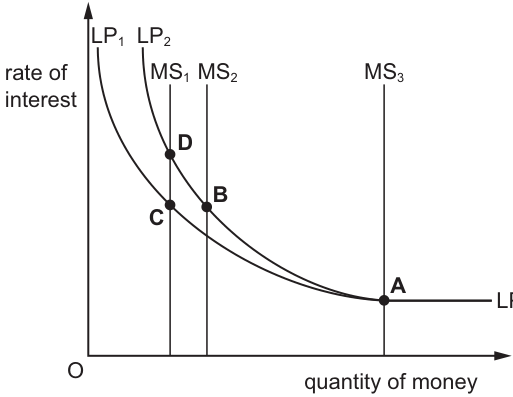
Sometimes monetary policy is ineffective. The supply of money (MS) is assumed to be controlled by the central bank. The demand for money is LP. There has been an increase in real income in the economy.
Which position on the diagram makes expansionary monetary policy ineffective?
Options
A point A on Fig. 14.1
B point B on Fig. 14.1
C point C on Fig. 14.1
D point D on Fig. 14.1
Working
Expansionary monetary policy increases the money supply to lower interest rates and boost aggregate demand. This is ineffective in a liquidity trap, where the demand for money is perfectly interest elastic (the horizontal section of the LP curve): any increase in the money supply is held as cash, so interest rates do not fall. Point A is on this horizontal section, so it is the position where expansionary monetary policy is ineffective.
Answer
A
A
Background Concept
This question is based on Keynesian liquidity preference theory, which models interest rate determination as the equilibrium between the supply of money (controlled by the central bank) and the demand for money (liquidity preference, LP). Money demand has three components: the transactions motive (money needed for daily purchases, which rises with real income), the precautionary motive (money held for unexpected expenses, also rising with income), and the speculative motive (money held to take advantage of future changes in bond prices, which falls as interest rates rise). At very low interest rates, people expect interest rates to rise in the future (and bond prices to fall), so they hold all their money as cash rather than buying bonds. This creates a horizontal section of the LP curve called the liquidity trap, where money demand is perfectly interest elastic.
Expansionary monetary policy works by the central bank increasing the money supply (shifting the MS curve right), which creates a surplus of money at the original interest rate. People use this surplus to buy bonds, pushing up bond prices and lowering the interest rate, until a new lower equilibrium is reached. Lower interest rates reduce borrowing costs, boosting investment and consumer spending on durables, which raises aggregate demand, real output and employment. However, this policy is ineffective in a liquidity trap, because the interest rate cannot fall below the lower bound: any extra money supply is held as cash, so interest rates do not fall, and spending is not stimulated.
Understanding the Question
The question asks which point on the provided liquidity preference diagram represents a position where expansionary monetary policy is ineffective, following an increase in real income in the economy. The diagram shows two LP curves: LP1 (original money demand) and LP2 (shifted right, representing higher money demand from the increase in real income). Three vertical money supply curves (MS1, MS2, MS3) and four equilibrium points (A, B, C, D) are marked. Point A lies on the horizontal (liquidity trap) section of the LP curve, while points B, C and D lie on the downward-sloping sections of the LP curve. The task is to identify which position makes expansionary monetary policy (increasing the money supply to lower interest rates) ineffective.
Approach
To solve this, first recall the mechanism of expansionary monetary policy in the liquidity preference model: it relies on increasing the money supply to lower the interest rate. The policy is only ineffective if the interest rate cannot fall when the money supply rises, which occurs only in the liquidity trap (the horizontal section of the LP curve). Next, identify which point is on this horizontal section, and confirm that the other points are on the downward-sloping section where money supply increases do lower interest rates. The increase in real income shifts the LP curve right, but this does not change the fact that the liquidity trap is the only position where monetary policy is ineffective.
Step-by-Step Reasoning
- First, confirm how expansionary monetary policy operates: when the central bank increases the money supply, the MS curve shifts right. At any point on the downward-sloping section of the LP curve, this creates a surplus of money at the original interest rate. People use the surplus to buy bonds, which raises bond prices and lowers the interest rate, until a new lower equilibrium is reached. The lower interest rate then stimulates investment and consumption, raising aggregate demand.
- The policy is ineffective only if the interest rate does not fall when the money supply increases. This occurs in the liquidity trap, the horizontal section of the LP curve, where the demand for money is perfectly interest elastic. In this region, people expect interest rates to rise in the future, so they hold all additional money as cash rather than buying bonds. The interest rate stays at the lower bound, so investment and consumption do not rise, and aggregate demand is unchanged.
- Now examine the positions on the diagram:
- Point A is on the horizontal (liquidity trap) section of the LP curve, at the intersection with MS3. If the economy is at point A, any increase in the money supply (e.g. shifting MS further right) will not lower the interest rate, so expansionary monetary policy is completely ineffective.
- Points B, C and D all lie on the downward-sloping sections of the LP curve. At these points, an increase in the money supply would create a surplus of money, lower the interest rate, and stimulate spending, so expansionary monetary policy is effective.
- The increase in real income mentioned in the question shifts the LP curve right from LP1 to LP2, but this does not alter the conclusion: the only position where monetary policy is ineffective is the liquidity trap at point A.
Key Takeaways
- The liquidity preference model explains interest rate determination as the equilibrium between money supply (set by the central bank) and money demand (driven by income and interest rates).
- Expansionary monetary policy works by increasing the money supply to lower interest rates and stimulate aggregate demand, but only when the LP curve is downward-sloping.
- The policy is ineffective in a liquidity trap, where the LP curve is horizontal (money demand is perfectly interest elastic) because any extra money supply is held as cash, so interest rates do not fall.
- An increase in real income shifts the LP curve right, raising the equilibrium interest rate at any given money supply, but does not eliminate the liquidity trap at the lower bound interest rate.
Common Mistakes
- Selecting points B, C or D: these lie on the downward-sloping section of the LP curve, where an increase in the money supply would lower interest rates and make monetary policy effective, so these are incorrect.
- Confusing the liquidity trap with a vertical money supply curve: the liquidity trap is a feature of the money demand (LP) curve, not the money supply curve.
- Misunderstanding the mechanism of ineffectiveness: monetary policy is not ineffective because the money supply cannot be increased, but because the increase does not lower interest rates to stimulate spending, which is the specific condition at point A.
- Ignoring the context of the question: the rightward shift of the LP curve from higher real income does not change which point represents the liquidity trap, as the horizontal section remains part of both LP1 and LP2.
Things to Be Careful About
- The horizontal section of the LP curve is explicitly labelled in the diagram, so point A is unambiguously the only point on this section.
- The question asks for the position where expansionary monetary policy is ineffective, not the outcome of the policy: point A is the starting equilibrium where any money supply increase will have no effect on interest rates.
- Remember that the liquidity trap occurs at very low interest rates, when the speculative demand for money is perfectly elastic: this is the only scenario in the Keynesian liquidity preference model where monetary policy is ineffective.
- Do not confuse the liquidity trap with a situation of fixed money supply: monetary policy ineffectiveness refers to the inability of changes in the money supply to affect interest rates, not the existence of the money supply curves themselves.
Which policy is most likely to lead to a reduction in the natural rate of unemployment?
Options
A an increase in government expenditure on goods and services
B an increase in government expenditure on training schemes to address skill shortages
C an increase in the period when the unemployed are eligible for welfare benefits
D an increase in the minimum wage
Answer
The natural rate of unemployment is the rate of unemployment that exists when the labour market is in equilibrium, consisting of frictional and structural unemployment. It is not affected by demand-side policies.
- A is a demand-side policy that reduces cyclical unemployment, not the natural rate.
- B directly reduces structural unemployment by addressing skill shortages, thereby lowering the natural rate.
- C increases the duration of benefit eligibility, which may increase frictional unemployment (by reducing the incentive to search for work) and thus raise the natural rate.
- D may increase structural unemployment if firms substitute capital for labour in response to higher labour costs, potentially raising the natural rate.
Therefore, the correct answer is B.
B
Background Concept
The natural rate of unemployment (also called the non-accelerating inflation rate of unemployment, NAIRU) is the rate of unemployment that prevails when the labour market is in equilibrium and there is no cyclical unemployment. It consists of:
- Frictional unemployment: workers between jobs, searching for the best match.
- Structural unemployment: a mismatch between workers' skills and the skills demanded by employers, often due to technological change or geographical immobility.
The natural rate is determined by supply-side factors: the structure of the labour market, the efficiency of job matching, the level and duration of welfare benefits, the skill composition of the workforce, and the degree of labour market flexibility. Demand-side policies (fiscal or monetary) can reduce cyclical unemployment in the short run but cannot permanently lower the natural rate.
Understanding the Question
This is a multiple-choice question asking which policy is most likely to reduce the natural rate of unemployment. The four options are all government policies, but they affect different types of unemployment. The key is to recognise that only supply-side policies that improve labour market efficiency or reduce structural/frictional mismatches can lower the natural rate.
Approach
For each option, determine whether it affects the natural rate (structural/frictional) or cyclical unemployment. Eliminate demand-side policies and policies that increase frictional or structural unemployment. The correct answer is the one that directly addresses a cause of the natural rate.
Step-by-Step Reasoning
- Option A: Increasing government expenditure on goods and services is a fiscal expansion that boosts aggregate demand. This reduces cyclical unemployment (demand-deficient) but does not change the underlying structural or frictional unemployment. The natural rate is unaffected.
- Option B: Training schemes address skill shortages, which are a cause of structural unemployment. By improving the match between workers' skills and available jobs, they reduce the duration and level of structural unemployment. This directly lowers the natural rate.
- Option C: Extending the period of welfare benefit eligibility reduces the incentive for unemployed workers to search actively for a job, increasing frictional unemployment. This raises the natural rate, not reduces it.
- Option D: An increase in the minimum wage may price low-skilled workers out of the labour market, leading to higher structural unemployment (if firms hire fewer workers or substitute capital for labour). This could increase the natural rate.
Thus, only option B is a supply-side policy that reduces the natural rate.
Key Takeaways
- The natural rate of unemployment is determined by supply-side factors, not aggregate demand.
- Policies that improve labour market flexibility, training, or job matching can lower the natural rate.
- Demand-side policies (fiscal/monetary) affect cyclical unemployment but not the natural rate.
- Welfare benefits and minimum wage increases can raise the natural rate by increasing frictional or structural unemployment.
Common Mistakes
- Confusing the natural rate with cyclical unemployment: thinking that any policy that reduces unemployment overall must reduce the natural rate.
- Not distinguishing between demand-side and supply-side policies.
- Assuming that increasing benefits always helps the unemployed; it can actually increase frictional unemployment.
Things to Be Careful About
- The question asks for the policy most likely to reduce the natural rate. Even if a policy has ambiguous effects (e.g., minimum wage could have small positive effects in some models), the clear answer is the training scheme.
- Remember that the natural rate is a long-run concept; short-run demand management does not affect it.
On a diagram showing a production possibility curve, what definitely represents long-run economic growth?
Options
A a change in the slope of the curve
B a movement from a point below the curve to a point on the curve
C a movement from one point to another along a given curve
D an outward shift of the curve
Answer
Long-run economic growth is an increase in the economy's productive capacity, meaning it can produce more goods and services than before. On a production possibility curve (PPC), this is shown by an outward shift of the curve. Option D is correct.
Option A (a change in the slope) represents a change in the opportunity cost ratio, not growth. Option B (a movement from below the curve to a point on the curve) represents a reduction in unemployed resources, which is actual growth (a movement towards potential output), not an increase in potential output itself. Option C (a movement along the curve) represents a reallocation of resources between the two goods, not growth.
Answer
D
D
Background Concept
A production possibility curve (PPC) shows the maximum combinations of two goods or services that an economy can produce using all its available resources efficiently. The curve represents the economy's potential output. Any point on the curve is productively efficient; any point inside the curve is inefficient (resources are underutilised).
Long-run economic growth refers to an increase in the economy's productive capacity — the ability to produce more goods and services in the future. This is also called potential growth. It comes from increases in the quantity or quality of factors of production (land, labour, capital, enterprise) or from improvements in technology that raise productivity.
Understanding the Question
The question asks which change on a PPC diagram definitely represents long-run economic growth. The key word is "definitely" — the answer must be unambiguous and always true. The four options describe different possible changes on a PPC diagram. The candidate must know what each change means and whether it necessarily indicates an increase in productive capacity.
Approach
Recall the distinction between:
- Potential growth (an increase in the economy's maximum possible output) — shown by an outward shift of the PPC.
- Actual growth (an increase in output from using previously idle resources) — shown by a movement from a point inside the curve to a point on the curve.
Then evaluate each option against this distinction.
Step-by-Step Reasoning
Option A: a change in the slope of the curve
The slope of the PPC represents the opportunity cost of producing one good in terms of the other. A change in slope means the trade-off has changed (e.g., because of technological progress in one sector but not the other). This could be associated with growth in one sector, but it does not definitely represent an overall increase in productive capacity. The curve could shift outwards in an uneven way, changing the slope, but a change in slope alone is not a reliable indicator of growth. So A is incorrect.
Option B: a movement from a point below the curve to a point on the curve
This represents a reduction in unemployed resources — the economy moves from an inefficient point (inside the PPC) to an efficient point (on the PPC). This is actual growth (an increase in output), but it does not increase the economy's maximum potential output. The PPC itself has not shifted. So B is not long-run economic growth.
Option C: a movement from one point to another along a given curve
This represents a reallocation of resources between the two goods. The economy produces more of one good and less of the other, but total output is still at the maximum possible given the same resources. There is no increase in productive capacity. So C is incorrect.
Option D: an outward shift of the curve
An outward shift means the economy can now produce more of both goods than before, using the same or better resources. This is the standard textbook representation of long-run (potential) economic growth. It is unambiguous and always true. So D is correct.
Key Takeaways
- Long-run (potential) economic growth is an increase in the economy's productive capacity, shown by an outward shift of the PPC.
- Actual growth (using idle resources) is shown by a movement from inside the PPC to a point on the PPC.
- A movement along the PPC is a change in the composition of output, not growth.
- A change in the slope of the PPC reflects a change in opportunity costs, not necessarily overall growth.
Common Mistakes
- Confusing actual growth (movement towards the PPC) with potential growth (outward shift of the PPC).
- Thinking that any movement on the diagram represents growth — only an outward shift of the curve itself does.
- Misinterpreting a change in slope as growth, when it may simply reflect a change in relative costs.
Things to Be Careful About
- The question says "definitely" — choose the option that is always true, not just sometimes associated with growth.
- Remember that the PPC represents maximum potential output, not actual output. An outward shift increases that maximum.
- A movement from inside to on the curve is an improvement in efficiency, not an increase in capacity.
The diagram shows equilibrium in the money market at point X.
If there is an increase in the level of income in the economy, which point shows the new equilibrium in the short term?
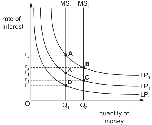
Options
A point A on Fig. 17.1
B point B on Fig. 17.1
C point C on Fig. 17.1
D point D on Fig. 17.1
Answer
An increase in income raises the transactions demand for money, shifting the liquidity preference curve to the right. Because the money supply (MS1) is fixed in the short run, the equilibrium interest rate rises while the quantity of money stays at Q1. The new equilibrium is therefore at point A.
A
A
Background Concept
The money market is analysed using the liquidity preference theory, where the rate of interest is determined by the equilibrium between the supply of money and the demand for money (liquidity preference). The supply of money (MS) in the short run is assumed to be fixed by the central bank, so it is represented by a vertical curve. The demand for money is inversely related to the rate of interest because interest is the opportunity cost of holding money. This demand comprises three motives: the transactions motive (which depends directly on income), the precautionary motive, and the speculative motive. When income rises, the transactions demand for money increases at every interest rate, shifting the entire liquidity preference (LP) curve to the right. With a fixed money supply, this excess demand for money bids up the interest rate until a new equilibrium is reached at a higher rate of interest but the same quantity of money.
Understanding the Question
The question provides a money market diagram showing an initial equilibrium at point X, where the money supply curve MS1 intersects the liquidity preference curve LP1 at interest rate r1 and quantity Q1. It asks which point represents the new short-run equilibrium after an increase in the level of income. The key phrase is "in the short term," which signals that the money supply is fixed (the central bank has not yet changed MS). We must identify the effect of higher income on money demand and then locate the corresponding new intersection on the diagram.
Approach
- Identify the direction of the shift in the liquidity preference curve: an increase in income raises money demand, so LP shifts rightward (from LP1 towards LP2 or LP3).
- Note that the money supply remains MS1 in the short run.
- The new equilibrium must lie on MS1 (fixed supply) at a higher interest rate than r1, because the rightward shift in LP creates excess demand for money at the original rate.
- Examine the points: Point A is on MS1 at a higher rate r3 and quantity Q1. Points B and C are on MS2, implying a change in money supply rather than money demand. Point D is on MS1 but at a lower rate r5, which would result from a decrease in money demand.
- Conclude that point A is the correct new equilibrium.
Step-by-Step Reasoning
- Initial equilibrium: The economy starts at point X where MS1 meets LP1. The interest rate is r1 and the quantity of money is Q1.
- Effect of higher income: When income increases, households and firms need more money for transactions (buying goods, paying wages, etc.). This increases the demand for money at every interest rate.
- Shift in the LP curve: The liquidity preference curve shifts to the right (for example, from LP1 to LP2). This is a shift of the entire curve, not a movement along it.
- Fixed money supply: In the short term, the central bank has not altered the money supply, so the supply curve remains MS1 (vertical at Q1).
- New equilibrium: The rightward shift in LP means that at the original interest rate r1, there is now excess demand for money. This competition for money pushes the interest rate upward. The market clears where the new LP curve intersects MS1. This occurs at a higher interest rate (r3) but the same quantity Q1, because the supply of money is fixed at Q1.
- Identification of point A: Point A is located at the intersection of MS1 and a higher LP curve (LP2) at interest rate r3 and quantity Q1. This matches the predicted new equilibrium.
- Why the other points are incorrect:
- Point B lies on MS2, which represents an increase in the money supply, not a change in income.
- Point C also lies on MS2, again implying a change in money supply rather than money demand.
- Point D lies on MS1 but at a lower interest rate r5. This would occur if money demand fell (a leftward shift of LP), which is the opposite of what happens when income rises.
Key Takeaways
- In the short run, the money supply is fixed by the central bank and is represented by a vertical curve.
- Income is a key determinant of the demand for money (via the transactions motive).
- An increase in income shifts the liquidity preference curve to the right.
- With a fixed money supply, a rightward shift in money demand raises the equilibrium interest rate but leaves the quantity of money unchanged.
- Always distinguish between a shift in a curve (caused by an external factor like income) and a movement along a curve (caused by a change in the variable on the axis, such as the interest rate).
Common Mistakes
- Confusing money supply and money demand: Selecting points B or C, which involve MS2. An increase in income affects demand, not supply. The money supply only changes if the central bank acts.
- Thinking the quantity of money changes: With a fixed MS, the quantity is determined by supply. The interest rate is the variable that adjusts to clear the market. Point A correctly keeps quantity at Q1.
- Reversing the direction of the shift: Picking point D, which would result from a fall in income (leftward LP shift), not a rise.
- Forgetting the short-run assumption: In the long run, the central bank might accommodate the higher demand, but the question explicitly asks for the short-term effect.
Things to Be Careful About
- The vertical axis is the rate of interest; the horizontal axis is the quantity of money.
- MS curves are vertical in the short run; LP curves are downward sloping.
- An increase in income shifts the LP curve to the right (higher demand), not left.
- The new equilibrium must lie on the original MS curve (MS1) because the money supply has not changed.
- Point A is the only point on MS1 that shows a higher interest rate than the initial equilibrium, which is the necessary outcome of increased money demand against fixed supply.
Which combination of policies is most likely to reduce cyclical unemployment but might increase frictional unemployment?
Options
| direct taxes | unemployment benefits | |
|---|---|---|
| A | decrease | decrease |
| B | decrease | increase |
| C | increase | decrease |
| D | increase | increase |
Answer
Cyclical unemployment is caused by a deficiency of aggregate demand. Reducing direct taxes raises disposable income, boosting consumption and aggregate demand, which reduces cyclical unemployment. Frictional unemployment arises from the time workers spend searching for jobs. Increasing unemployment benefits reduces the opportunity cost of job search, lengthening the time workers spend looking for work and thus increasing frictional unemployment. The combination that achieves both effects is a decrease in direct taxes and an increase in unemployment benefits.
Answer
B
B
Background Concept
Unemployment is categorised into several types, each with different causes. Cyclical unemployment (also called demand-deficient or Keynesian unemployment) occurs when there is insufficient aggregate demand in the economy to employ all those willing to work at the current wage rate. It rises during recessions and falls during booms. Frictional unemployment is the short-term unemployment that occurs when workers are between jobs, searching for new positions that better match their skills and preferences. It is a natural and inevitable part of a dynamic economy, but its duration can be influenced by policy.
Fiscal policy uses government spending and taxation to influence aggregate demand. A cut in direct taxes (income tax, corporation tax) increases households' disposable income and firms' post-tax profits, stimulating consumption and investment, which raises aggregate demand and reduces cyclical unemployment. Supply-side policies aim to improve the functioning of labour markets. Unemployment benefits affect the incentive to search for work: higher benefits reduce the cost of being unemployed, potentially lengthening job search and increasing frictional unemployment.
Understanding the Question
The question asks for a combination of two policy changes — one to direct taxes and one to unemployment benefits — that would MOST LIKELY reduce cyclical unemployment but MIGHT increase frictional unemployment. This is a policy trade-off question. You must trace the effect of each policy change on each type of unemployment and find the row in the table where the two effects match the stated outcome.
Approach
- Identify what reduces cyclical unemployment: a policy that boosts aggregate demand. A cut in direct taxes does this. An increase in direct taxes would reduce demand and worsen cyclical unemployment.
- Identify what increases frictional unemployment: a policy that lengthens job search. Higher unemployment benefits reduce the urgency to find a new job, increasing frictional unemployment. Lower benefits would shorten search and reduce frictional unemployment.
- Find the row where direct taxes are decreased (to reduce cyclical unemployment) AND unemployment benefits are increased (to increase frictional unemployment). That is row B.
Step-by-Step Reasoning
Step 1: Effect of direct taxes on cyclical unemployment
- Cyclical unemployment is caused by a shortfall in aggregate demand (AD).
- A decrease in direct taxes leaves households with more disposable income. This increases consumption (C), a component of AD (AD = C + I + G + X - M).
- Higher AD shifts the AD curve rightwards. If the economy is operating below full employment (with a negative output gap), this increases real output and employment, reducing cyclical unemployment.
- An increase in direct taxes would have the opposite effect: lower disposable income, lower consumption, lower AD, and higher cyclical unemployment.
- Therefore, to reduce cyclical unemployment, direct taxes must be decreased. This eliminates options C and D (which increase direct taxes).
Step 2: Effect of unemployment benefits on frictional unemployment
- Frictional unemployment is the time spent searching for a new job.
- Unemployment benefits provide income to workers while they are unemployed. Higher benefits reduce the financial pressure to accept the first available job, allowing workers to search longer for a better match.
- This longer search period increases the measured frictional unemployment rate.
- Lower benefits would increase the opportunity cost of remaining unemployed, encouraging workers to accept jobs more quickly, reducing frictional unemployment.
- Therefore, to increase frictional unemployment, unemployment benefits must be increased. This eliminates option A (which decreases benefits).
Step 3: Select the correct combination
- The only remaining option that decreases direct taxes AND increases unemployment benefits is option B.
Key Takeaways
- Different types of unemployment have different causes and therefore respond to different policies.
- A single policy can have opposite effects on different types of unemployment. A cut in direct taxes reduces cyclical unemployment but has no direct effect on frictional unemployment. Higher benefits increase frictional unemployment but do not directly affect cyclical unemployment.
- Policy evaluation often involves trade-offs: the combination that helps one objective may worsen another.
Common Mistakes
- Confusing cyclical with structural unemployment. Structural unemployment is caused by a mismatch of skills or location, not by deficient demand, and would not be reduced by a tax cut alone.
- Thinking that higher unemployment benefits always increase unemployment. They increase frictional unemployment (by lengthening search) but can also reduce the pressure to accept a job below one's skill level, potentially improving labour market matching in the long run.
- Selecting option A (decrease both) because it seems 'pro-growth'. Decreasing benefits would reduce frictional unemployment, not increase it, so it fails the second condition.
- Selecting option D (increase both) because it seems 'generous'. Increasing taxes would worsen cyclical unemployment, failing the first condition.
Things to Be Careful About
- Read the question carefully: it asks for the combination that reduces cyclical unemployment BUT MIGHT increase frictional unemployment. Both conditions must be satisfied.
- Distinguish between the direct effect of a policy and its indirect or long-run effects. The question asks for the most likely direct effect.
- Remember that frictional unemployment is not necessarily bad; some frictional unemployment is efficient as it allows better job matching. The question simply asks which policy combination would increase it.
What would cause the short-run Phillips curve to shift to the right?
Options
A the unemployment rate is above the natural rate of unemployment, decreasing inflationary expectations
B the unemployment rate is above the natural rate of unemployment, increasing inflationary expectations
C the unemployment rate is below the natural rate of unemployment, decreasing inflationary expectations
D the unemployment rate is below the natural rate of unemployment, increasing inflationary expectations
Answer
The short-run Phillips curve shifts to the right when inflationary expectations increase. This occurs when the actual unemployment rate is below the natural rate, as this creates upward pressure on wages and prices, leading workers and firms to revise their expectations of inflation upwards. Therefore, the correct answer is D.
D
Background Concept
The Phillips curve illustrates the inverse relationship between the rate of unemployment and the rate of inflation. In the short run, this trade-off exists because nominal wages are sticky. The expectations-augmented Phillips curve (EAPC) incorporates the role of inflationary expectations. The equation is:
Inflation rate = Expected inflation rate - b(Unemployment rate - Natural rate of unemployment) + Supply shocks
Where 'b' is a positive constant measuring the responsiveness of inflation to the unemployment gap. The short-run Phillips curve (SRPC) is drawn for a given level of expected inflation. When expected inflation changes, the SRPC shifts.
Understanding the Question
This question asks what would cause the short-run Phillips curve to shift to the right. A rightward shift means that for any given unemployment rate, the inflation rate is higher. The options link this shift to two conditions: (1) whether the actual unemployment rate is above or below the natural rate, and (2) whether inflationary expectations are decreasing or increasing. The key is to identify which combination of these conditions leads to higher expected inflation, which is the direct cause of a rightward SRPC shift.
Approach
- Recall the determinant of the SRPC's position: expected inflation.
- Determine what causes expected inflation to rise. This happens when actual inflation persistently exceeds what was expected, which occurs when the economy is overheating (unemployment below the natural rate).
- Match this to the options: unemployment below the natural rate AND increasing inflationary expectations.
Step-by-Step Reasoning
- The short-run Phillips curve shows the relationship between unemployment and inflation for a given expected inflation rate.
- A rightward shift of the SRPC means that at every unemployment rate, the inflation rate is higher. This is caused by an increase in inflationary expectations.
- When the actual unemployment rate is below the natural rate, the economy is operating beyond its potential. This creates demand-pull inflation as firms compete for scarce labour, pushing up wages and prices.
- If this situation persists, workers and firms will revise their expectations of future inflation upwards. They will demand higher nominal wages to maintain real wages, and firms will raise prices in anticipation of higher costs.
- This increase in expected inflation shifts the short-run Phillips curve to the right.
- Option D states: "the unemployment rate is below the natural rate of unemployment, increasing inflationary expectations." This exactly matches the reasoning.
- Options A and B describe a situation where unemployment is above the natural rate. This would put downward pressure on inflation, likely decreasing inflationary expectations and shifting the SRPC to the left, not the right.
- Option C describes unemployment below the natural rate but with decreasing inflationary expectations. This is contradictory; below-natural unemployment typically increases, not decreases, inflationary expectations.
Key Takeaways
- The position of the short-run Phillips curve is determined by expected inflation.
- An increase in expected inflation shifts the SRPC to the right (higher inflation for any given unemployment rate).
- A decrease in expected inflation shifts the SRPC to the left.
- The actual unemployment rate relative to the natural rate influences whether expected inflation is rising or falling.
Common Mistakes
- Confusing a movement along the SRPC with a shift of the SRPC. A change in the actual unemployment rate causes a movement along the curve, not a shift. A shift is caused by a change in expected inflation.
- Thinking that any deviation of unemployment from the natural rate directly shifts the SRPC. It is the resulting change in inflationary expectations that causes the shift, not the deviation itself.
- Selecting option B (unemployment above natural rate, increasing expectations). This is incorrect because above-natural unemployment would reduce inflation, likely decreasing expectations.
Things to Be Careful About
- Distinguish between the short-run and long-run Phillips curves. The long-run Phillips curve is vertical at the natural rate of unemployment, and shifts only when the natural rate itself changes.
- Remember that the "rightward shift" of the SRPC means higher inflation at each unemployment rate. This is equivalent to an upward shift in the traditional Phillips curve diagram (inflation on the vertical axis, unemployment on the horizontal axis).
Which macroeconomic policy is most likely to be used as a long-run means of reducing inflationary pressures?
Options
A exchange rate policy
B fiscal policy
C supply-side policy
D monetary policy
Answer
Supply-side policy is most likely to be used as a long-run means of reducing inflationary pressures. It aims to increase the productive capacity of the economy, shifting the long-run aggregate supply (LRAS) curve to the right. This reduces the general price level sustainably without relying on demand management that may cause unemployment. In contrast, exchange rate, fiscal, and monetary policies primarily manage aggregate demand in the short run and can have adverse side effects such as higher unemployment or currency volatility.
C
Background Concept
Inflation is a sustained increase in the general price level. Policies to reduce it fall into two broad categories: demand-side policies (monetary, fiscal, and exchange rate) which reduce aggregate demand (AD), and supply-side policies which increase aggregate supply (AS). Demand-side policies work by cooling the economy, often at the cost of higher unemployment and lower output in the short run. Supply-side policies address the root cause of cost-push inflation by improving productivity, competition, and efficiency, thereby lowering costs and expanding the economy's potential output without sacrificing employment.
Understanding the Question
The question asks which macroeconomic policy is most likely to be used as a long-run means of reducing inflationary pressures. The key phrase is "long-run" — this signals that the policy should address the structural causes of inflation rather than merely suppressing demand temporarily. The four options are exchange rate policy, fiscal policy, supply-side policy, and monetary policy. The correct answer is C (supply-side policy).
Approach
To answer, we need to evaluate each option against the criterion of long-run effectiveness. Monetary and fiscal policies are demand-management tools that work in the short run but can cause unemployment or be ineffective if inflation is cost-push. Exchange rate policy can reduce imported inflation but is not a long-run solution. Supply-side policy directly increases the economy's productive capacity, reducing inflationary pressures sustainably.
Step-by-Step Reasoning
- Monetary policy (D): Central banks raise interest rates to reduce AD. This can lower demand-pull inflation but may cause unemployment and is not effective against cost-push inflation. It is a short-run tool.
- Fiscal policy (B): The government reduces spending or raises taxes to reduce AD. Again, this is a short-run demand-side measure with potential negative effects on output and employment.
- Exchange rate policy (A): A government might appreciate the currency to reduce import prices, lowering cost-push inflation. However, this can harm exports and is not a sustainable long-run strategy.
- Supply-side policy (C): Policies such as deregulation, tax reforms, investment in education and infrastructure, and promoting competition increase LRAS. This reduces the price level sustainably and can also boost employment and growth.
Thus, supply-side policy is the most appropriate long-run solution.
Key Takeaways
- Distinguish between demand-side (short-run) and supply-side (long-run) policies.
- Supply-side policies address the root causes of inflation by expanding productive capacity.
- Demand-side policies can reduce inflation but often at the cost of higher unemployment.
Common Mistakes
- Choosing monetary policy because it is the most common tool used by central banks, without considering the "long-run" qualifier.
- Confusing exchange rate policy as a long-run solution when it is typically a short-run adjustment.
- Not recognising that supply-side policy is the only option that directly increases AS.
Things to Be Careful About
- Read the question carefully: "long-run" is the decisive qualifier.
- Understand that supply-side policy is not a quick fix but a structural reform.
- Remember that demand-side policies can be used in the long run too, but they are less effective and have undesirable side effects compared to supply-side measures.
The table identifies pairs of possible government aims. The achievement of aim 1 needs to be consistent with the achievement of aim 2.
Which row shows the combination where both aims are likely to be achieved.
Options
| aim 1 | aim 2 | |
|---|---|---|
| A | higher foreign exchange rate | lower rate of unemployment |
| B | low rate of inflation | current account surplus |
| C | more even distribution of income | higher rate of saving |
| D | rapid economic growth | sustainable economic development |
Answer
B
B
Background Concept
Macroeconomic objectives are the broad goals governments pursue to manage the economy. Common objectives include low inflation, low unemployment, economic growth, a stable balance of payments, and a more equitable distribution of income. However, these objectives can conflict with each other, meaning that achieving one may make it harder to achieve another. For example, policies to boost growth may cause inflation, or policies to reduce inflation may increase unemployment. This question tests the ability to identify which pair of aims are consistent — that is, where achieving aim 1 helps or at least does not hinder achieving aim 2.
Understanding the Question
The question presents four rows (A–D), each pairing two government aims. The task is to select the row where achieving aim 1 is likely to be consistent with achieving aim 2. The table is:
| aim 1 | aim 2 | |
|---|---|---|
| A | higher foreign exchange rate | lower rate of unemployment |
| B | low rate of inflation | current account surplus |
| C | more even distribution of income | higher rate of saving |
| D | rapid economic growth | sustainable economic development |
We need to evaluate each pair for consistency.
Approach
For each row, consider the economic relationship between the two aims. Ask: does achieving aim 1 tend to help achieve aim 2, or does it create a conflict? Eliminate rows where the aims are likely to conflict. The correct row is the one where both aims can be achieved together, or where achieving one supports the other.
Step-by-Step Reasoning
Row A: higher foreign exchange rate (aim 1) and lower rate of unemployment (aim 2)
A higher foreign exchange rate means the domestic currency appreciates. This makes exports more expensive and imports cheaper. As a result, net exports (X – M) are likely to fall, reducing aggregate demand (AD). Lower AD tends to reduce output and increase unemployment. Therefore, a higher exchange rate is likely to increase unemployment, not lower it. These aims conflict. Eliminate A.
Row B: low rate of inflation (aim 1) and current account surplus (aim 2)
Low inflation makes a country's goods more price-competitive internationally compared to countries with higher inflation. This tends to boost exports and reduce imports, improving the current account balance. A current account surplus means exports exceed imports. Thus, low inflation supports a current account surplus. These aims are consistent. B is a strong candidate.
Row C: more even distribution of income (aim 1) and higher rate of saving (aim 2)
A more even distribution of income typically means lower-income households receive a larger share. Lower-income households have a higher marginal propensity to consume (MPC) and a lower marginal propensity to save (MPS) than higher-income households. Redistributing income from rich to poor is therefore likely to reduce the overall saving rate, not increase it. These aims conflict. Eliminate C.
Row D: rapid economic growth (aim 1) and sustainable economic development (aim 2)
Rapid economic growth often involves high resource consumption, pollution, and environmental degradation, which can undermine sustainability. Sustainable development aims to meet present needs without compromising future generations. Rapid growth may conflict with sustainability unless it is managed carefully. While some forms of growth can be sustainable, the phrase "rapid economic growth" typically implies a pace that is difficult to sustain environmentally. These aims are likely to conflict. Eliminate D.
Therefore, only row B shows a combination where both aims are likely to be achieved together.
Key Takeaways
- Macroeconomic objectives can conflict; understanding the trade-offs is essential.
- Low inflation improves international competitiveness, supporting a current account surplus.
- Redistribution of income tends to reduce saving because lower-income groups save less.
- Rapid growth often conflicts with environmental sustainability.
- A higher exchange rate tends to worsen the current account and increase unemployment.
Common Mistakes
- Assuming that a higher exchange rate is always good for the economy — it actually harms export competitiveness and can raise unemployment.
- Thinking that a more even income distribution automatically increases saving — the opposite is true because the poor save less.
- Confusing "sustainable economic development" with "economic growth" — they are not the same, and rapid growth can be unsustainable.
- Not considering the indirect effects: for example, low inflation helps the current account through competitiveness, not directly.
Things to Be Careful About
- Read the table carefully: aim 1 is the first column, aim 2 is the second. The question asks for consistency between achieving aim 1 and aim 2.
- "Higher foreign exchange rate" means appreciation, not depreciation.
- "Current account surplus" is a positive balance on trade in goods and services.
- "Sustainable economic development" includes environmental and intergenerational equity, not just growth.
The central bank of an economy decreases the money supply in an attempt to reduce inflation.
Under which conditions is this policy most likely to be effective?
Options
| exchange rate | responsiveness of aggregate demand to interest rate changes | |
|---|---|---|
| A | fixed | low |
| B | fixed | high |
| C | floating | low |
| D | floating | high |
Answer
A decrease in the money supply raises interest rates. Higher interest rates reduce investment and consumption, lowering aggregate demand and, eventually, the price level. This transmission mechanism works only if aggregate demand is highly responsive to interest rate changes.
Under a floating exchange rate, higher interest rates also attract capital inflows, causing the currency to appreciate. The appreciation reduces net exports, reinforcing the contractionary effect on AD. Under a fixed exchange rate, the central bank would have to sell foreign reserves to prevent the appreciation, which would expand the money supply again, partially or fully offsetting the initial contraction.
Therefore, the policy is most effective when the exchange rate is floating and the responsiveness of AD to interest rates is high.
Answer
D
D
Background Concept
This question tests the transmission mechanism of monetary policy and how it is affected by the exchange rate regime. The core idea is that a contractionary monetary policy (reducing the money supply) works through two channels:
-
Interest rate channel: A smaller money supply raises interest rates (the price of money). Higher interest rates increase the cost of borrowing, which reduces consumption (especially of durable goods) and investment spending. This lowers aggregate demand (AD) and, if sustained, reduces inflationary pressure.
-
Exchange rate channel: Higher interest rates attract foreign capital seeking higher returns. This increases demand for the domestic currency, causing it to appreciate. A stronger currency makes exports more expensive and imports cheaper, reducing net exports (X-M), which further reduces AD.
Under a floating exchange rate, the currency is free to appreciate, so both channels operate fully. Under a fixed exchange rate, the central bank must intervene to maintain the peg: it sells foreign reserves to buy domestic currency, which prevents the appreciation but also reduces the money supply further (sterilised intervention is possible but imperfect). More importantly, if the central bank is committed to the fixed rate, it may have to expand the money supply later to counteract the appreciation pressure, undermining the original contraction.
Understanding the Question
The question asks: under which combination of exchange rate system (fixed or floating) and responsiveness of AD to interest rate changes (low or high) is a contractionary monetary policy most likely to be effective?
- "Effectiveness" here means the policy successfully reduces inflation by lowering AD.
- The two variables are: (1) the exchange rate regime, and (2) the interest rate sensitivity of AD.
- We need to identify the combination where both channels work in the same direction and the policy is not offset.
Approach
- Identify the transmission mechanism of monetary policy.
- Consider how a floating exchange rate reinforces the policy (appreciation reduces net exports).
- Consider how a fixed exchange rate can offset the policy (intervention to maintain the peg may reverse the money supply change).
- Consider the role of interest rate sensitivity: if AD is unresponsive to interest rates, the interest rate channel is weak, so even with a floating rate the policy may be ineffective.
- The most effective combination is floating + high responsiveness.
Step-by-Step Reasoning
Step 1: The interest rate channel
- Money supply decreases -> interest rates rise (assuming money demand is stable).
- Higher interest rates increase the cost of borrowing for firms (investment) and households (consumption, especially mortgages and car loans).
- If AD is highly responsive to interest rates, the fall in investment and consumption is large, so AD falls significantly, reducing inflation.
- If AD is unresponsive (low responsiveness), the same interest rate rise produces only a small fall in AD, so the policy is weak.
Step 2: The exchange rate channel under floating rates
- Higher interest rates attract foreign capital inflows (hot money).
- Demand for the domestic currency rises, causing it to appreciate.
- Appreciation makes exports more expensive in foreign currency and imports cheaper in domestic currency.
- Net exports (X-M) fall, reducing AD further.
- This reinforces the interest rate channel, making the policy more effective.
Step 3: The exchange rate channel under fixed rates
- The central bank is committed to maintaining a fixed exchange rate.
- Higher interest rates attract capital inflows, putting upward pressure on the currency.
- To prevent appreciation, the central bank must sell domestic currency and buy foreign reserves. This increases the money supply, partially or fully offsetting the initial contraction.
- Alternatively, the central bank could sterilise the intervention (sell bonds to absorb the extra liquidity), but this is imperfect and may signal a lack of commitment.
- Therefore, under a fixed rate, the exchange rate channel does not reinforce the policy; it may even undermine it.
Step 4: Combining the conditions
- Option A (fixed + low): The interest rate channel is weak, and the fixed rate prevents the exchange rate channel from working. Least effective.
- Option B (fixed + high): The interest rate channel works, but the fixed rate may offset it. Effectiveness is limited.
- Option C (floating + low): The exchange rate channel works (appreciation reduces net exports), but the interest rate channel is weak. Some effect, but limited.
- Option D (floating + high): Both channels work fully. The interest rate channel directly reduces AD, and the appreciation reinforces it. Most effective.
Step 5: Conclusion
The policy is most effective when the exchange rate is floating (so the appreciation channel operates) and AD is highly responsive to interest rate changes (so the interest rate channel is strong). This corresponds to option D.
Key Takeaways
- Monetary policy works through interest rates and exchange rates.
- A floating exchange rate reinforces monetary policy (appreciation adds to the contraction).
- A fixed exchange rate can undermine monetary policy (intervention may reverse the money supply change).
- The effectiveness of monetary policy depends on how responsive spending is to interest rate changes.
- This question illustrates the "impossible trinity" (or trilemma): a country cannot simultaneously have a fixed exchange rate, independent monetary policy, and free capital flows.
Common Mistakes
- Confusing fixed and floating: Some students think a fixed rate makes monetary policy more effective because the exchange rate is stable. In fact, it reduces policy autonomy.
- Ignoring the exchange rate channel: Students may only consider the interest rate channel and miss that the exchange rate regime matters.
- Assuming low responsiveness is better: Some think that if AD is unresponsive, the policy is more effective because it doesn't cause a recession. But the question asks about reducing inflation, not avoiding side effects.
- Not reading the table carefully: The table has two columns: exchange rate and responsiveness. Option D is "floating" and "high".
Things to Be Careful About
- The question asks for the condition under which the policy is most likely to be effective, not the only condition.
- "Responsiveness of aggregate demand to interest rate changes" is the same as the interest rate sensitivity of investment and consumption.
- Under a fixed exchange rate with perfect capital mobility, monetary policy is completely ineffective (the trilemma). This question assumes some capital mobility but not perfect.
- The exchange rate channel works through net exports, which depends on the Marshall-Lerner condition (whether the sum of export and import demand elasticities exceeds one). The question implicitly assumes this holds.
A government reduces both the income tax paid by all earners and the amount of means-tested benefits paid to those receiving low or no incomes.
What is most likely to be its objective?
Options
A a more equitable income distribution
B a reduction in the rate of inflation
C a reduction in the trade deficit
D an increase in the rate of economic growth
Answer
Reducing income tax raises the post-tax reward for working, increasing the incentive to supply labour. Reducing means-tested benefits removes the poverty trap (the high effective marginal tax rate when benefits are withdrawn as earnings rise), further strengthening the incentive to work. Together these policies increase the quantity and quality of labour supplied, raising the economy's productive potential and the rate of economic growth. The objective is therefore an increase in the rate of economic growth.
Answer
D
D
Background Concept
This question tests understanding of the poverty trap and how tax and benefit reforms can affect labour supply and economic growth. The poverty trap occurs when means-tested benefits are withdrawn as a person's income rises, creating a high effective marginal tax rate (the combined loss of benefit and payment of tax on additional earnings). This reduces the financial incentive to work more or to seek higher-paid employment. Cutting income tax and reducing means-tested benefits both lower the effective marginal tax rate, encouraging labour supply. Increased labour supply raises the economy's productive capacity (potential output) and, if aggregate demand is sufficient, can lead to higher actual growth.
Understanding the Question
The question describes two simultaneous policy changes: a reduction in income tax for all earners, and a reduction in the amount of means-tested benefits paid to those with low or no incomes. The task is to identify the most likely objective of this combination. The four options are: a more equitable income distribution, a reduction in inflation, a reduction in the trade deficit, and an increase in economic growth. The key is to recognise that cutting benefits reduces equity (makes the distribution less equal), so option A is unlikely. The other options require considering the macroeconomic effects.
Approach
First, analyse the direct effect of each policy separately. Income tax cuts increase disposable income and the reward for working, boosting labour supply and aggregate demand. Benefit cuts reduce disposable income for the poorest, which may reduce aggregate demand but also strengthen work incentives by reducing the poverty trap. The combined effect on labour supply is unambiguously positive (both policies increase the incentive to work). Increased labour supply raises potential output and, if demand is maintained, actual growth. Inflation and the trade deficit are less directly affected and the net effect on them is ambiguous. Therefore, the most likely objective is to increase economic growth.
Step-by-Step Reasoning
-
Income tax cut: Reduces the tax wedge between what employers pay and what workers receive. Workers keep more of each additional pound earned, so the opportunity cost of leisure rises. This increases the quantity of labour supplied (both more hours and more people entering the workforce). Higher labour supply shifts the aggregate supply curve rightwards, increasing potential output.
-
Benefit cut: Means-tested benefits are withdrawn as income rises. This creates a high effective marginal tax rate (the 'poverty trap'). Reducing the amount of benefit paid reduces the withdrawal rate (or the amount withdrawn), lowering the effective marginal tax rate. This further strengthens the incentive to work, especially for those previously trapped in low-paid or part-time work. Again, labour supply increases.
-
Combined effect on labour supply: Both policies work in the same direction — they increase the net financial gain from working. The labour supply curve shifts right. This is a supply-side policy aimed at increasing the productive capacity of the economy.
-
Effect on economic growth: With more labour available, the economy can produce more goods and services. If aggregate demand is maintained (the tax cut may boost consumption and investment), actual output rises. Even if demand falls slightly (due to benefit cuts reducing spending by the poor), the increase in potential output means the economy can grow faster in the long run. The most direct and likely objective is therefore to increase the rate of economic growth.
-
Why not the other options?
- A (more equitable distribution): Cutting benefits reduces the income of the poorest, making the distribution less equal. The tax cut may benefit higher earners more in absolute terms. So equity worsens.
- B (reduction in inflation): The effect on inflation is ambiguous. Increased labour supply reduces cost-push pressures, but the tax cut may boost demand. The net effect is uncertain and not the primary aim.
- C (reduction in trade deficit): The effect on the trade deficit is also ambiguous. Higher growth may increase imports, worsening the deficit. There is no direct link to the trade balance.
Key Takeaways
- The poverty trap is a key concept linking tax and benefit policy to labour supply.
- Supply-side policies aim to increase the productive capacity of the economy.
- Cutting benefits can improve work incentives but worsens equity — there is often a trade-off.
- When evaluating policy objectives, consider the direct and most likely effect, not every possible indirect consequence.
Common Mistakes
- Choosing A because 'cutting tax and benefits helps the poor' — but cutting benefits actually hurts the poor, so equity is not improved.
- Confusing the poverty trap with absolute poverty. The poverty trap is about incentives, not just low income.
- Thinking that cutting benefits always reduces aggregate demand and therefore growth — but the supply-side effect on labour supply can dominate.
- Not recognising that both policies together strengthen work incentives more than either alone.
Things to Be Careful About
- Read the question carefully: it says 'most likely' objective, not 'only possible' objective. Some policies have multiple effects, but one is the primary aim.
- Distinguish between equity (fairness) and equality (sameness). Cutting benefits reduces both.
- Remember that supply-side policies often have a lag before they affect growth, but the objective is still growth.
What is not a likely feature of a customs union?
Options
A common external tariffs with non-member nations
B elimination of tariffs between member nations
C elimination of quotas between member nations
D shared common currency among member nations
Answer
A customs union involves the elimination of internal tariffs (B) and quotas (C) between member nations, and the adoption of a common external tariff (A) against non-members. A shared common currency (D) is a feature of a monetary union, not a customs union. Therefore, D is not a likely feature of a customs union.
Answer
D
D
Background Concept
Economic integration refers to the process by which countries reduce trade barriers and coordinate their economic policies. There are several stages of integration, each adding more features:
- Free Trade Area (FTA): Members eliminate tariffs and quotas on trade among themselves, but each member maintains its own separate trade policies (including tariffs) towards non-members.
- Customs Union: All features of an FTA, PLUS members adopt a common external tariff (CET) on imports from non-members. This prevents trade deflection (where goods enter the union through the member with the lowest tariff).
- Common Market (Single Market): All features of a customs union, PLUS free movement of factors of production (labour and capital) between members.
- Monetary Union: All features of a common market, PLUS members share a common currency and a common central bank (e.g., the Eurozone).
- Full Economic Union: All features of a monetary union, PLUS harmonisation of fiscal and other economic policies.
Understanding the Question
This is a multiple-choice question asking which of the four listed features is not a likely feature of a customs union. The question tests your knowledge of the precise characteristics that define a customs union, as distinct from other forms of integration. You need to identify the one option that belongs to a deeper stage of integration (monetary union) rather than to a customs union.
Approach
- Recall the defining features of a customs union: elimination of internal tariffs and quotas, plus a common external tariff.
- Check each option against this definition.
- Identify the option that is not part of a customs union — that is, the one that belongs to a higher stage of integration.
Step-by-Step Reasoning
- Option A: Common external tariffs with non-member nations. This is a core feature of a customs union. It prevents trade deflection and ensures a unified trade policy. This IS a feature.
- Option B: Elimination of tariffs between member nations. This is the basic starting point of any preferential trade agreement, including a customs union. This IS a feature.
- Option C: Elimination of quotas between member nations. Quotas are non-tariff barriers; their removal is also part of the internal liberalisation within a customs union. This IS a feature.
- Option D: Shared common currency among member nations. A common currency is a feature of a monetary union (e.g., the Eurozone), which goes beyond a customs union. A customs union does not require members to give up their national currencies. This is NOT a feature of a customs union.
Therefore, the correct answer is D.
Key Takeaways
- Know the hierarchy of economic integration: Free Trade Area → Customs Union → Common Market → Monetary Union → Full Economic Union.
- Each stage adds specific features; a customs union is defined by internal free trade PLUS a common external tariff.
- A common currency belongs to a monetary union, not a customs union.
Common Mistakes
- Confusing a customs union with a free trade area (forgetting the common external tariff).
- Confusing a customs union with a monetary union (thinking a common currency is included).
- Not reading the question carefully: it asks for what is not a likely feature, so students may mistakenly pick a feature that IS present.
Things to Be Careful About
- Read the question stem carefully — "What is not a likely feature..." — to avoid selecting a true feature.
- Distinguish clearly between the different stages of integration; memorise the key additions at each stage.
A central bank officially lowers the price of its currency relative to an agreed rate in terms of other currencies.
What type of central bank policy is this?
Options
A appreciation
B depreciation
C devaluation
D revaluation
Answer
A central bank officially lowering the price of its currency relative to an agreed rate describes a devaluation. This occurs under a fixed exchange rate system, where the government or central bank sets an official parity and then deliberately reduces it. Depreciation, by contrast, is a market-driven fall in a floating exchange rate.
Answer
C
C
Background Concept
Exchange rates can be determined in two broad ways: floating (market forces of demand and supply set the rate) and fixed (the government or central bank pegs the currency at a specific value against another currency or a basket of currencies). Under a fixed system, the official parity is an announced target. If the central bank decides to lower that target, it is called a devaluation. If it raises the target, it is a revaluation. Under a floating system, a fall in the market price of the currency is called a depreciation, and a rise is an appreciation.
Understanding the Question
The question describes a deliberate, official action by a central bank to lower the price of its currency relative to an agreed rate. The key phrase is "officially lowers" and "relative to an agreed rate" — this tells you the exchange rate is not freely floating but is managed or fixed. The question asks you to identify the correct term for this policy.
Approach
- Identify the exchange rate regime implied by "agreed rate" — this points to a fixed or managed system.
- Recall the vocabulary: devaluation = official reduction in a fixed rate; depreciation = market-driven fall in a floating rate.
- Eliminate the options that describe the opposite direction (appreciation, revaluation) or the wrong regime (depreciation).
Step-by-Step Reasoning
- Option A: appreciation — This is an increase in the value of a currency under a floating system. The question says "lowers the price", so this is the opposite direction. Incorrect.
- Option B: depreciation — This is a fall in the value of a currency under a floating exchange rate system. The question mentions an "agreed rate", which implies a fixed or managed system, not a free float. Incorrect.
- Option C: devaluation — This is the correct term for an official reduction in the value of a currency under a fixed exchange rate system. The central bank sets a new, lower parity. Correct.
- Option D: revaluation — This is an official increase in the value of a currency under a fixed system. The question says "lowers", so this is the opposite. Incorrect.
Therefore, the correct answer is C.
Key Takeaways
- The distinction between devaluation/depreciation (fall in value) and revaluation/appreciation (rise in value) depends on the exchange rate regime.
- "Official" or "agreed rate" signals a fixed system; "market forces" signal a floating system.
- Memorise the four terms and their regime contexts.
Common Mistakes
- Confusing devaluation with depreciation: both mean a fall in value, but devaluation is official under fixed rates, depreciation is market-driven under floating rates.
- Choosing "depreciation" because the question says "lowers the price" without noticing the "agreed rate" clue.
- Mixing up devaluation (down) with revaluation (up).
Things to Be Careful About
- Always read the full description: "officially lowers" and "agreed rate" are the decisive clues.
- Remember that under a managed float, the central bank may intervene to influence the rate, but an official change in the parity is still called a devaluation/revaluation if the system has a fixed element.
Which combination of events would cause the biggest increase in real GDP per capita?
Options
| GDP | population | general price level | |
|---|---|---|---|
| A | rises | falls | falls |
| B | rises | falls | rises |
| C | rises | rises | falls |
| D | rises | rises | rises |
Answer
Real GDP per capita is calculated as (Nominal GDP / Price Level) / Population. To maximise the increase, we want:
- Nominal GDP to rise (increases the numerator).
- The price level to fall (deflation increases the real value of GDP).
- Population to fall (fewer people to share the output).
Option A is the only combination where all three move in the direction that increases real GDP per capita: GDP rises, population falls, and the price level falls. In options B, C and D at least one of the three moves in the wrong direction (price level rises in B and D; population rises in C and D), reducing or offsetting the increase.
A
A
Background Concept
Real GDP per capita is a key monetary indicator of living standards. It adjusts nominal GDP for two factors: inflation (to get real GDP) and population size (to get per capita). The formula is:
Real GDP per capita = (Nominal GDP / GDP Deflator) / Population
Or equivalently: Real GDP per capita = Real GDP / Population
Where Real GDP = Nominal GDP adjusted for changes in the general price level. A fall in the price level (deflation) increases the purchasing power of nominal GDP, so real GDP rises even if nominal GDP stays constant. A rise in population means the same output must be shared among more people, reducing per capita income.
Understanding the Question
The question asks which combination of changes to three variables — GDP (nominal), population, and the general price level — would produce the biggest increase in real GDP per capita. Each option shows whether each variable rises or falls. We need to evaluate how each change affects the final ratio.
Approach
- Identify the formula for real GDP per capita.
- For each variable, determine whether a rise or fall increases or decreases the final value.
- Compare the four options: the one where all three changes push in the same direction (towards a higher value) will produce the biggest increase.
Step-by-Step Reasoning
Step 1: The formula
Real GDP per capita = (Nominal GDP / Price Level) / Population
- A rise in Nominal GDP increases the numerator -> increases the result.
- A fall in the Price Level (deflation) means the denominator of the first division is smaller, so Real GDP is larger -> increases the result.
- A fall in Population means the denominator of the second division is smaller -> increases the result.
Step 2: Evaluate each option
| Option | GDP | Population | Price Level | Effect on Real GDP per capita |
|---|---|---|---|---|
| A | rises | falls | falls | All three changes increase the value -> biggest increase |
| B | rises | falls | rises | GDP rise and population fall help, but price level rise reduces real GDP -> net increase smaller than A |
| C | rises | rises | falls | GDP rise and price level fall help, but population rise reduces per capita value -> net increase smaller than A |
| D | rises | rises | rises | Only GDP rise helps; population rise and price level rise both reduce the value -> smallest increase (possibly even a decrease) |
Step 3: Conclusion
Option A is the only one where all three variables move in the direction that increases real GDP per capita. Therefore it produces the biggest increase.
Key Takeaways
- Real GDP per capita is a composite measure requiring two adjustments: for inflation and for population.
- When comparing scenarios, identify whether each variable's change pushes the final value up or down.
- The biggest increase occurs when all relevant variables move in the favourable direction simultaneously.
Common Mistakes
- Confusing nominal GDP with real GDP: a rise in nominal GDP alone does not guarantee a rise in real GDP if prices rise faster.
- Forgetting the population adjustment: a rise in GDP per capita requires output to grow faster than population.
- Thinking a rise in the price level helps: inflation reduces the real value of nominal GDP.
Things to Be Careful About
- The question uses "GDP" without specifying nominal or real. In context, it means nominal GDP, because the price level adjustment is given separately.
- "General price level" is the GDP deflator or a price index; a fall means deflation.
- The question asks for the "biggest increase", not just an increase. Option A is the only one where all three changes are favourable, so it is unambiguously the largest.
A low-income country receives aid from a high-income country.
When will this aid give maximum benefit in the long term to the low-income country?
Options
| type of aid | purpose of the aid | |
|---|---|---|
| A | grant | purchase of agricultural machinery |
| B | grant | payment of food subsidies |
| C | loan | purchase of agricultural machinery |
| D | loan | payment of food subsidies |
Answer
A grant is a gift that does not need to be repaid, avoiding future debt repayment burdens. The purchase of agricultural machinery is a capital investment that raises the country's productive capacity and enables sustainable long-term growth. In contrast, a loan creates a future debt obligation, and food subsidies are a consumption transfer that provides only short-term relief without building productive assets. Therefore, the maximum long-term benefit comes from a grant used for the purchase of agricultural machinery.
Answer
A
A
Background Concept
International aid is a transfer of resources from one country (usually a high-income donor) to another (usually a low-income recipient). Aid can be classified by its form (grant or loan) and by its purpose (investment or consumption). A grant is a gift that does not require repayment, while a loan must be repaid with interest. The purpose of aid matters because investment in capital goods (machinery, infrastructure, education) increases the recipient's productive capacity and can generate self-sustaining growth, whereas consumption aid (food, medicine, subsidies) meets immediate needs but does not build long-term productive assets.
Understanding the Question
The question asks when aid gives maximum benefit in the long term to a low-income country. It presents a 2x2 matrix: the type of aid (grant vs loan) and the purpose of the aid (purchase of agricultural machinery vs payment of food subsidies). The correct answer is the combination that best promotes long-term development. The key is to evaluate each option against the criterion of long-term benefit, considering both the repayment burden and the nature of the expenditure.
Approach
- Evaluate the type of aid: Grants are superior to loans for long-term benefit because loans create a future debt burden that can crowd out other spending and reduce net benefit.
- Evaluate the purpose of aid: Investment in capital goods (agricultural machinery) is superior to consumption subsidies because it raises productivity and enables future growth, while subsidies provide only temporary relief.
- Combine the two criteria: The option that is both a grant and an investment (agricultural machinery) is the best for long-term benefit.
Step-by-Step Reasoning
- Option A (Grant + Agricultural machinery): A grant imposes no repayment obligation, so all of the aid's value is a net gain to the recipient. The machinery is a capital investment that increases agricultural productivity, leading to higher output, income, and potentially exports. This creates a sustainable source of growth and reduces future dependence on aid. This is the best for long-term development.
- Option B (Grant + Food subsidies): While the grant avoids debt, food subsidies are a consumption transfer. They help alleviate immediate hunger and poverty but do not build productive capacity. Once the aid stops, the benefit ends. There is no lasting increase in the country's ability to produce food or income.
- Option C (Loan + Agricultural machinery): The machinery is a good investment, but the loan must be repaid with interest. This creates a future debt burden that may require the country to divert resources from other development priorities (health, education) to service the debt. The net long-term benefit is reduced compared to a grant for the same purpose.
- Option D (Loan + Food subsidies): This is the worst combination. The loan creates a debt burden, and the subsidies are pure consumption with no lasting productive impact. The country ends up worse off in the long run, as it must repay the loan without having built any additional productive capacity.
Therefore, only Option A maximises long-term benefit.
Key Takeaways
- The form of aid (grant vs loan) matters because of the future repayment burden.
- The purpose of aid (investment vs consumption) determines whether it builds long-term productive capacity or provides only temporary relief.
- For sustainable development, aid should ideally be in the form of grants directed towards investment in capital goods, infrastructure, or human capital.
- This question tests the ability to apply economic reasoning about investment, debt, and long-term growth to a practical policy choice.
Common Mistakes
- Choosing a loan because it is 'larger' or 'more credible': The question asks for maximum long-term benefit, not short-term availability. Loans impose a future cost.
- Focusing only on the purpose and ignoring the type: Some students might pick Option C because machinery is good, forgetting that the loan reduces net benefit.
- Thinking food subsidies are investment: Subsidies are consumption; they do not raise the country's productive capacity.
- Overlooking the 'long term' qualifier: In the short term, food subsidies might save lives, but the question explicitly asks for long-term benefit.
Things to Be Careful About
- Read the question carefully: it asks for the combination that gives maximum benefit in the long term.
- Distinguish between consumption and investment: machinery is a capital good that yields future returns; subsidies are consumed immediately.
- Remember that loans must be repaid, reducing the net benefit of the aid.
- Do not confuse the purpose of aid with its form; both dimensions must be evaluated together.
Which variable is included in the calculation of both the Human Development Index (HDI) and the Multidimensional Poverty Index (MPI)?
Options
A child mortality rate
B gross national income (GNI) per capita
C life expectancy at birth
D years of schooling
Answer
The HDI is calculated from three dimensions: life expectancy at birth (health), expected years of schooling and mean years of schooling (education), and GNI per capita (standard of living). The MPI uses ten indicators across three dimensions: health (child mortality and nutrition), education (years of schooling and school attendance), and standard of living (cooking fuel, sanitation, water, electricity, floor, assets). The only variable common to both is years of schooling.
D
D
Background Concept
The Human Development Index (HDI) and the Multidimensional Poverty Index (MPI) are both composite indicators used to measure well-being beyond simple income measures. The HDI, published by the UNDP, focuses on average achievement in three basic dimensions: health (life expectancy at birth), education (expected years of schooling for school-age children and mean years of schooling for adults aged 25+), and standard of living (GNI per capita in PPP terms). The MPI, also from the UNDP, measures acute multidimensional poverty by looking at deprivations across the same three dimensions but using ten indicators: health (child mortality, nutrition), education (years of schooling, school attendance), and standard of living (cooking fuel, improved sanitation, safe drinking water, electricity, adequate housing floor, and asset ownership). A household is considered multidimensionally poor if it is deprived in at least one-third of the weighted indicators.
Understanding the Question
This is a straightforward multiple-choice question asking which single variable appears in the calculation of both the HDI and the MPI. The four options are: child mortality rate, GNI per capita, life expectancy at birth, and years of schooling. The question tests precise knowledge of the components of each index, not just a general understanding of what they measure.
Approach
Recall the exact components of the HDI and the MPI. For each option, check whether it is a component of both indices. The correct answer is the one that appears in both.
Step-by-Step Reasoning
- HDI components: The HDI is the geometric mean of three normalized indices:
- Health: life expectancy at birth
- Education: expected years of schooling (for children) and mean years of schooling (for adults)
- Standard of living: GNI per capita (PPP US$)
- MPI components: The MPI uses ten indicators grouped into three dimensions:
- Health: child mortality (whether any child has died in the household) and nutrition (whether any adult or child is undernourished)
- Education: years of schooling (whether no household member has completed at least six years of schooling) and school attendance (whether any school-age child is not attending school up to class 8)
- Standard of living: six indicators (cooking fuel, sanitation, water, electricity, floor, assets)
- Check each option:
- A child mortality rate: This is an indicator in the MPI (health dimension) but NOT a component of the HDI (which uses life expectancy at birth, not child mortality).
- B GNI per capita: This is a component of the HDI (standard of living dimension) but NOT a component of the MPI (which uses asset-based indicators for standard of living, not income).
- C life expectancy at birth: This is a component of the HDI (health dimension) but NOT a component of the MPI (which uses child mortality and nutrition, not life expectancy).
- D years of schooling: This is a component of the HDI (education dimension, as mean years of schooling) AND a component of the MPI (education dimension, as an indicator of deprivation). Therefore, it is the only variable common to both.
Key Takeaways
- The HDI measures average achievement; the MPI measures deprivation.
- Both indices cover health, education, and standard of living, but they use different specific indicators.
- The only overlapping variable is years of schooling (or education attainment).
- Knowing the exact components of composite indicators is essential for multiple-choice questions and for essay discussions of development measurement.
Common Mistakes
- Assuming that because both indices cover health, they use the same health indicator (life expectancy vs. child mortality/nutrition).
- Confusing the HDI's use of GNI per capita with the MPI's use of asset-based deprivation indicators.
- Thinking that child mortality is part of the HDI because it is a common development statistic.
Things to Be Careful About
- The HDI uses life expectancy at birth, not child mortality.
- The MPI uses years of schooling as a deprivation indicator (whether anyone has completed at least six years), while the HDI uses mean years of schooling for adults.
- The question asks for a variable included in the calculation of both indices, not just a concept they both relate to.
Which diagram is not an example of a Kuznets curve?
Options
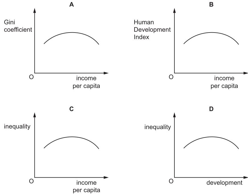
Answer
The Kuznets curve depicts an inverted U-shaped relationship between economic development (or income per capita) and income inequality. Diagrams A, C and D all show inequality (or the Gini coefficient, which measures inequality) on the vertical axis against income per capita or development on the horizontal axis, consistent with the Kuznets hypothesis. Diagram B shows the Human Development Index (HDI), which is a composite measure of development (including health and education), not a measure of inequality. HDI rises with income per capita and does not follow an inverted U-shape in the Kuznets sense. Therefore, B is not an example of a Kuznets curve.
B
Background Concept
The Kuznets curve is a hypothesis proposed by Simon Kuznets in the 1950s suggesting that as an economy develops, income inequality first increases and then decreases, creating an inverted U-shaped relationship when inequality is plotted against income per capita or the level of economic development. The vertical axis represents income inequality, commonly measured by the Gini coefficient (where 0 represents perfect equality and 1 represents perfect inequality). The horizontal axis represents economic development, typically measured by income per capita. In the early stages of development, industrialisation and the shift from agriculture to industry increase inequality as some sectors grow faster than others. As development continues, education spreads, labour markets become more inclusive, and redistribution policies often reduce inequality. The Human Development Index (HDI), by contrast, is a composite statistic of life expectancy, education, and per capita income indicators used to rank countries into tiers of human development. HDI generally increases monotonically with income per capita and does not exhibit an inverted U-shape.
Understanding the Question
The question asks which of the four diagrams is NOT an example of a Kuznets curve. This requires recognising the specific relationship the Kuznets curve depicts: an inverted U-shape showing how income inequality changes as income per capita or development increases. The candidate must examine the labels on the axes of each diagram to determine whether the relationship being shown matches the Kuznets hypothesis. The key distinction is between measures of inequality (Gini coefficient, inequality) on the vertical axis versus measures of development (HDI) on the vertical axis.
Approach
To answer this, evaluate each diagram against the definition of a Kuznets curve:
- Check if the vertical axis represents inequality (Gini coefficient or general inequality).
- Check if the horizontal axis represents income per capita or development.
- Confirm the curve is inverted U-shaped.
Diagrams A, C, and D fit this pattern. Diagram B uses HDI on the vertical axis, which is incorrect because HDI is a development indicator, not an inequality measure, and its relationship with income per capita is not an inverted U.
Step-by-Step Reasoning
- Diagram A: Shows the Gini coefficient (a precise measure of income inequality) on the vertical axis against income per capita on the horizontal axis, with an inverted U-shaped curve. This is the standard representation of the Kuznets curve. It qualifies as a Kuznets curve.
- Diagram B: Shows the Human Development Index (HDI) on the vertical axis against income per capita on the horizontal axis. HDI is a composite index measuring average achievement in key dimensions of human development (health, education, and living standards). While HDI is related to income, it is not a measure of inequality. Moreover, HDI tends to rise with income per capita, not fall after an initial rise. Therefore, this does not represent a Kuznets curve.
- Diagram C: Shows inequality on the vertical axis against income per capita on the horizontal axis, with an inverted U-shape. This is a general representation of the Kuznets curve using generic labels. It qualifies.
- Diagram D: Shows inequality on the vertical axis against development on the horizontal axis. Since development is often proxied by income per capita, this is another valid representation of the Kuznets curve. It qualifies.
Since the question asks which is NOT an example, the answer is B.
Key Takeaways
- The Kuznets curve specifically models the relationship between economic development/income and income inequality.
- The vertical axis must represent inequality (Gini coefficient or general inequality).
- The horizontal axis represents income per capita or level of development.
- The curve is inverted U-shaped.
- HDI is a measure of development achievement, not inequality, and does not follow the Kuznets pattern.
Common Mistakes
- Confusing HDI with a measure of inequality. HDI includes health and education outcomes and generally increases with income.
- Assuming any inverted U-shaped curve in development economics is a Kuznets curve without checking the axis labels.
- Failing to notice that the Kuznets curve is specifically about the distribution of income (inequality), not the level of development itself.
Things to Be Careful About
- Always check the vertical axis label: it must be an inequality measure (Gini coefficient or inequality).
- The horizontal axis can be income per capita or development.
- The Kuznets curve predicts inequality rises then falls with development; HDI simply rises with development.
- In multiple-choice questions, eliminate the three correct examples first, then select the remaining option.
The table shows the value of the Gini coefficient for an economy from 2018 to 2020.
| year | Gini coefficient |
|---|---|
| 2018 | 0.29 |
| 2019 | 0.28 |
| 2020 | 0.27 |
What is most likely to explain the change in the value of the Gini coefficient between 2018 and 2020?
Options
A an increase in indirect taxes
B an increase in long-term unemployment
C an increase in the national minimum wage
D an increase in population
Answer
The Gini coefficient fell from 0.29 to 0.27 between 2018 and 2020, indicating a reduction in income inequality. An increase in the national minimum wage (option C) would raise the incomes of the lowest-paid workers, compressing the distribution and lowering the Gini coefficient. The other options would either increase inequality (A, B) or have no clear effect on the Gini coefficient (D).
Answer
C
C
Background Concept
The Gini coefficient is a summary measure of income (or wealth) inequality within a country. It ranges from 0 (perfect equality, where everyone has the same income) to 1 (perfect inequality, where one person has all the income). A falling Gini coefficient means the distribution of income is becoming more equal. The Lorenz curve is the graphical representation: the closer the curve is to the 45-degree line of perfect equality, the lower the Gini coefficient.
Understanding the Question
The table shows the Gini coefficient for an economy falling from 0.29 to 0.27 over three years. The question asks which of four events is most likely to explain this reduction in inequality. The task is to reason about the likely effect of each event on the distribution of incomes, not just on the average income or on the level of economic activity.
Approach
Evaluate each option in turn, asking: would this event tend to make the income distribution more equal (lower Gini) or less equal (higher Gini)?
- A: Increase in indirect taxes – Indirect taxes (e.g. VAT, sales tax) are regressive: they take a larger proportion of income from lower-income households, who spend a higher share of their income. This would likely widen inequality, raising the Gini coefficient.
- B: Increase in long-term unemployment – Long-term unemployment concentrates income loss among those already at the bottom of the distribution, widening the gap between the employed and the unemployed. This would raise the Gini coefficient.
- C: Increase in the national minimum wage – A higher minimum wage directly raises the earnings of the lowest-paid workers. If it does not cause significant job losses, it compresses the lower tail of the income distribution, reducing inequality and lowering the Gini coefficient.
- D: Increase in population – Population growth alone, without any change in the distribution of income, does not directly affect the Gini coefficient. The coefficient is a measure of relative inequality, not absolute numbers. A larger population could be associated with many different distributional changes, but by itself it provides no reason for the Gini to fall.
Only option C provides a clear mechanism for a sustained reduction in inequality over the period.
Step-by-Step Reasoning
-
Interpret the data: The Gini coefficient fell from 0.29 to 0.27. This is a meaningful decline, indicating that the income distribution became more equal.
-
Evaluate option A: An increase in indirect taxes raises the prices of goods and services. Lower-income households spend a larger fraction of their income on consumption, so they bear a disproportionate burden. This increases the effective inequality of disposable income, raising the Gini coefficient. Therefore, A is inconsistent with the observed fall.
-
Evaluate option B: An increase in long-term unemployment means more people have little or no labour income. Since the unemployed are typically at the bottom of the income distribution, this widens the gap between them and the employed, increasing inequality and raising the Gini coefficient. Therefore, B is inconsistent with the observed fall.
-
Evaluate option C: An increase in the national minimum wage raises the hourly earnings of the lowest-paid workers. If the minimum wage is binding (i.e. set above the market-clearing wage for low-skilled labour), it directly increases the incomes of those at the bottom of the distribution. This compresses the lower tail of the income distribution, reducing the Gini coefficient. The effect is strongest if employment does not fall significantly. Therefore, C is consistent with the observed fall.
-
Evaluate option D: An increase in population, by itself, does not change the relative distribution of income. The Gini coefficient is scale-invariant: doubling the population while keeping the relative income shares the same leaves the Gini unchanged. Population growth could be associated with many other changes (e.g. immigration of low-skilled workers, which might increase inequality), but the option states only an increase in population, with no further information. Therefore, D provides no clear explanation for the fall.
-
Conclusion: Only option C offers a plausible mechanism for a reduction in income inequality over the period.
Key Takeaways
- The Gini coefficient measures relative inequality, not absolute income levels.
- A falling Gini coefficient means the income distribution is becoming more equal.
- Policies that raise the incomes of the lowest-paid (e.g. a higher minimum wage, progressive taxes, means-tested benefits) tend to lower the Gini coefficient.
- Regressive taxes (e.g. indirect taxes) and increases in unemployment tend to raise the Gini coefficient.
- Population growth alone does not change the Gini coefficient.
Common Mistakes
- Confusing the Gini coefficient with a measure of average income or economic growth. A country can have rising average income and a rising Gini (more inequality) at the same time.
- Assuming that any 'good' economic change (like population growth) must reduce inequality. Population growth has no direct effect on the distribution.
- Thinking that an increase in the minimum wage always reduces inequality without considering possible employment effects. The question asks for the 'most likely' explanation, and the standard textbook effect is a reduction in inequality.
Things to Be Careful About
- The Gini coefficient is a relative measure: it is not affected by proportional changes in all incomes (e.g. all incomes doubling leaves the Gini unchanged).
- The question asks for the 'most likely' explanation, not the only possible one. In the real world, many factors affect inequality simultaneously, but the exam expects the clearest causal link.
- Indirect taxes are regressive, but the degree of regressivity depends on the specific goods taxed. The standard assumption in A-Level economics is that indirect taxes are regressive.
Your score so far
Answer a question to start scoring
Your marks add up here as you work through the paper.