Economics 9708/31 — October/November 2025
Cambridge A-Level · A Level Multiple Choice · answer key with instant marking and worked solutions
Topics Money and Banking · Exchange Rate Systems · Government Policies to Correct Market Failure · Balance of Payments and Policies to Correct Disequilibrium · Efficiency and Market Failure · Externalities, Social Costs and Benefits · +16 more
Tap an option under each question to check it — your score builds as you go.
What is likely to lead to the principal-agent problem?
Options
A a manager of a business makes decisions on behalf of the owner
B music festival tickets are purchased by a person who intends to sell them at a large profit
C the government is the only buyer of a pharmaceutical product
D there is only one firm that manufactures the product
Answer
The principal-agent problem arises when the agent (e.g. a manager) makes decisions on behalf of the principal (e.g. the owner) but has different objectives, leading to a conflict of interest. Option A describes exactly this situation: a manager acting for the owner.
Answer
A
A
Background Concept
The principal-agent problem is a key concept in the economics of organisations. It occurs when one party (the principal) hires another party (the agent) to make decisions on their behalf, but the agent's interests do not perfectly align with the principal's. The agent may pursue their own goals (e.g., higher salary, job security, prestige) rather than maximising the principal's welfare (e.g., profit for the owner). This is a form of market failure arising from asymmetric information and incomplete contracts.
Understanding the Question
This is a multiple-choice question asking which scenario is likely to lead to the principal-agent problem. The question tests your ability to recognise the core condition: a separation of ownership and control, where one person (the agent) acts for another (the principal) and has discretion to pursue their own interests.
Approach
Read each option and ask: does this involve a principal-agent relationship? The key is that one party is authorised to act on behalf of another, and their interests may diverge. Eliminate options that describe other economic phenomena (speculation, monopsony, monopoly).
Step-by-Step Reasoning
- Option A: A manager (agent) makes decisions for the owner (principal). The manager may prioritise sales growth, job perks, or risk avoidance over profit maximisation. This is the classic principal-agent problem. Correct.
- Option B: A person buys tickets to resell at a profit. This is speculation or arbitrage, not a principal-agent relationship. The buyer acts for themselves, not for another. Incorrect.
- Option C: The government is the only buyer (monopsony). This describes market structure, not a principal-agent problem. Incorrect.
- Option D: Only one firm produces the product (monopoly). Again, market structure, not a principal-agent relationship. Incorrect.
Key Takeaways
- The principal-agent problem requires a separation of ownership and control, with the agent having discretion to act for the principal.
- It is distinct from market structures (monopoly, monopsony) and from speculative behaviour.
- Common examples: managers vs. shareholders, politicians vs. voters, doctors vs. patients.
Common Mistakes
- Confusing the principal-agent problem with monopoly or monopsony. These are about market power, not about conflicting objectives within a relationship.
- Thinking any situation where one person benefits at another's expense is the principal-agent problem. The key is the agency relationship — one party is authorised to act for another.
Things to Be Careful About
- The question asks what is likely to lead to the problem. Option A is the only one that describes the necessary conditions.
- Do not overcomplicate: the definition is straightforward.
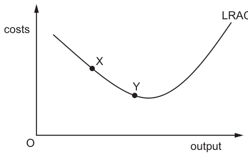
A small European airline currently produces at point X on its long-run average cost curve (LRAC). It wants a bigger share of the European airline market and proposes to merge with another small European airline. The newly merged firm would produce at point Y on the long-run average cost curve, as shown.
Why might the newly merged firm be able to produce at point Y?
Options
A The new airline can negotiate discounts when buying fuel.
B The new airline has many layers of management.
C The new airline is unable to hire enough pilots.
D The workforce of the new airline lacks morale and is demotivated.
Answer
The merger increases the scale of output, allowing the firm to move from point X to point Y on the long-run average cost (LRAC) curve. Point Y represents a higher output and lower average cost, indicating economies of scale. Option A is correct because negotiating discounts when buying fuel is an example of an internal economy of scale (purchasing economies). As the merged firm buys fuel in larger quantities, it can secure lower per-unit costs, enabling production at point Y.
A
Background Concept
In the long run, all factors of production are variable, and a firm can adjust its scale of output. The long-run average cost (LRAC) curve is typically U-shaped, reflecting how average costs change as output expands. The downward-sloping portion of the LRAC curve represents economies of scale: as output increases, average cost falls. This occurs because larger firms can spread fixed costs over more units, benefit from specialized labour and machinery, and secure purchasing discounts from suppliers. The lowest point of the LRAC represents minimum efficient scale (MES), the output level at which average costs are minimized. Beyond this point, the curve slopes upward, reflecting diseconomies of scale—for example, bureaucratic inefficiencies, coordination problems, or low worker morale—where further expansion raises average costs.
Economies of scale can be internal (arising from the growth of the individual firm, such as purchasing, technical, or managerial economies) or external (arising from industry-wide growth, such as improved infrastructure or a skilled local labour pool). The question describes a merger between two airlines, which is a form of integration that increases the size of the individual firm, making internal economies of scale the relevant concept.
Understanding the Question
The question presents a scenario where a small European airline currently operates at point X on the downward-sloping section of its LRAC curve. After merging with another airline, the firm would produce at point Y, which is further down the curve: higher output and lower average cost. The question asks why this merger enables the firm to reach point Y.
This is a 1-mark multiple-choice question. The candidate must recognize that:
- Movement from X to Y is a movement down the LRAC curve.
- This represents a fall in average cost as output rises.
- This is the definition of economies of scale.
- The correct answer must identify a factor that lowers average costs as the firm grows larger.
The diagram shows the LRAC curve with costs on the vertical axis and output on the horizontal axis. Point X is on the downward-sloping section; point Y is at a higher output and lower cost, closer to the minimum point.
Approach
The strategy is straightforward:
- Identify the economic meaning of the movement from X to Y: economies of scale.
- Evaluate each option to determine whether it describes a factor that would lower average costs (an economy of scale) or raise them (a diseconomy or constraint).
- Select the option that correctly explains the cost reduction.
Option A describes purchasing economies (bulk buying discounts), a classic internal economy of scale. Options B, C, and D describe factors associated with diseconomies of scale or constraints that would increase costs or prevent expansion, making them inconsistent with the movement to point Y.
Step-by-Step Reasoning
Analysis of the diagram and scenario:
Point X is on the downward-sloping portion of the LRAC curve, meaning the firm is currently experiencing economies of scale. Point Y is at a higher output level and lower average cost, closer to the minimum efficient scale. The merger increases the firm's scale of operations, allowing it to exploit economies of scale that were unavailable when it was smaller. The question asks for the reason this movement is possible.
Evaluation of Option A:
Fuel is a significant cost for airlines. When the airline merges with another, its total fuel consumption increases substantially. This larger volume gives the merged firm greater bargaining power when negotiating with fuel suppliers. Suppliers are likely to offer discounts for large, reliable orders because the transaction value is higher and the buyer is more important to the supplier. This reduces the average cost per unit of fuel, contributing to lower overall average costs. This is an internal economy of scale—specifically, a purchasing economy. This directly explains why the merged firm can produce at point Y.
Evaluation of Option B:
Having many layers of management is a classic symptom of diseconomies of scale. As firms grow larger, they often develop complex bureaucratic structures with multiple management tiers. This can slow decision-making, create communication problems, and increase administrative costs. These factors would shift the firm's LRAC upward or prevent it from reaching lower-cost points, making this option inconsistent with the movement to point Y.
Evaluation of Option C:
Being unable to hire enough pilots is a resource constraint in the factor market. This would prevent the firm from expanding output to the level associated with point Y. Alternatively, to attract scarce pilots, the firm might have to offer higher wages, which would increase average costs. This option does not explain lower average costs.
Evaluation of Option D:
Low workforce morale and demotivation typically reduce labour productivity (output per worker) and may increase absenteeism and turnover. This raises unit labour costs and represents X-inefficiency or a diseconomy of scale. It would not enable the firm to reach point Y.
Conclusion:
Only Option A provides a valid economic explanation for why the merged firm can achieve lower average costs at higher output. The merger creates purchasing economies of scale.
Key Takeaways
- The LRAC curve shows the relationship between a firm's scale of output and its average cost in the long run.
- Movement down the LRAC curve (from X to Y) represents economies of scale.
- Internal economies of scale include purchasing economies (bulk buying discounts), technical economies, managerial economies, and financial economies.
- Mergers and integration enable firms to grow larger and exploit internal economies of scale.
- Diseconomies of scale (bureaucracy, low morale, resource shortages) increase average costs and would move the firm up the LRAC curve.
Common Mistakes
- Confusing economies and diseconomies of scale: Students may be tempted by options B, C, or D because mergers can indeed create management challenges or integration problems. However, the question specifically asks why the firm can produce at point Y (lower cost), so only a cost-reducing factor is correct.
- Misinterpreting the diagram: Failing to recognize that point Y represents lower average cost and higher output than point X, and therefore represents economies of scale rather than diseconomies.
- Ignoring the context: The question is about a merger (a form of external growth), which increases firm size. The answer must relate to the benefits of increased size, not general business problems.
Things to Be Careful About
- Ensure you read the question carefully: it asks why the firm can produce at point Y (lower cost), not what problems the merger might cause.
- Distinguish between internal and external economies of scale. Option A is an internal economy (arising from the firm's own expansion via merger). External economies would come from industry-wide growth, which is not relevant here.
- In multiple-choice questions, eliminate options that describe cost increases or constraints first, as they cannot explain movement to a lower-cost point on the LRAC curve.
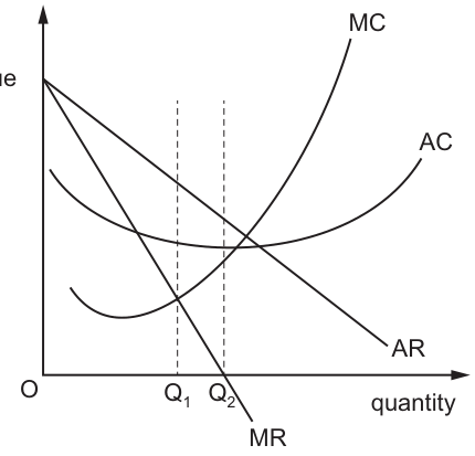
The diagram shows that a producer increases output from Q1 to Q2.
What will be the result?
Options
| total profit | total revenue | |
|---|---|---|
| A | increased | increased |
| B | increased | reduced |
| C | reduced | increased |
| D | reduced | reduced |
Answer
Output Q1 is where MC = MR, the profit-maximizing level. Increasing output to Q2 means producing units where MC > MR, so total profit falls.
Total revenue increases because the firm moves from Q1 towards the revenue-maximizing output (where MR = 0). Although MR becomes negative at Q2, the gain in revenue from the additional units sold while MR is still positive outweighs the loss from the negative marginal revenue, resulting in higher total revenue at Q2 than at Q1.
Answer
C
C
Background Concept
A firm with market power (such as a monopolist or monopolistic competitor) faces a downward-sloping average revenue (AR) curve and a steeper downward-sloping marginal revenue (MR) curve. The firm maximizes profit where marginal cost (MC) equals marginal revenue (MR). At this point, producing one more unit would add more to cost than to revenue, while producing one less unit would mean missing out on profitable sales.
Total revenue (TR) is maximized at a different point: where MR = 0. To the left of this point, MR is positive and TR is increasing as output rises. To the right, MR is negative and TR is falling. Total profit is the difference between total revenue and total cost (TC). Because the profit-maximizing output (where MC = MR) typically occurs where MR is still positive (and demand is price-elastic), the revenue-maximizing output is to the right of the profit-maximizing output.
Understanding the Question
The diagram shows a firm producing at Q1, where the MC curve intersects the MR curve. This is the profit-maximizing output. The question asks what happens when the firm increases output to Q2. The diagram indicates that Q2 is to the right of Q1 and that the MR curve has crossed the horizontal axis (become negative) by Q2.
The question tests whether you understand:
- That moving away from the profit-maximizing output reduces profit.
- How total revenue changes when moving from the profit-maximizing output towards and beyond the revenue-maximizing output.
The options pair changes in total profit with changes in total revenue. The correct combination is that profit falls while revenue rises.
Approach
First, identify Q1 as the profit-maximizing output because MC = MR there. Any movement away from this point reduces profit. Since Q2 > Q1 and MC is upward-sloping while MR is downward-sloping, at Q2 we have MC > MR, confirming profit falls.
Second, analyze total revenue. At Q1, MR is positive (since MC is positive and MC = MR). This means demand is elastic at Q1 and TR is still increasing as output rises. The revenue-maximizing point is where MR = 0, which lies between Q1 and Q2 according to the diagram. Even though MR is negative at Q2, total revenue at Q2 is higher than at Q1 because the firm has moved closer to the revenue-maximizing output. The positive marginal revenue from the initial extra units (between Q1 and the MR = 0 point) adds more to total revenue than the negative marginal revenue beyond that point subtracts.
Step-by-Step Reasoning
Step 1: Identify the profit-maximizing output.
The diagram shows the MC curve intersecting the MR curve at output Q1. This is the defining condition for profit maximization: produce where MC = MR. At this output, the firm cannot increase profit by changing output.
Step 2: Determine the change in total profit.
When the firm increases output from Q1 to Q2, it produces additional units. Because MC is upward-sloping and MR is downward-sloping, at any output greater than Q1, MC exceeds MR. This means each additional unit costs more to produce than the revenue it generates. Consequently, total profit falls. The firm moves down the profit hill away from the maximum.
Step 3: Determine the change in total revenue.
Total revenue changes according to the marginal revenue of the additional units. From Q1 to the point where MR = 0 (the revenue-maximizing output), MR is positive, so TR increases. Beyond that point, MR is negative, so TR decreases. Since Q2 lies to the right of Q1 but the MR = 0 point lies between them, the change in TR from Q1 to Q2 depends on the net area under the MR curve between these outputs.
At Q1, MR is positive, meaning the firm is on the elastic portion of the demand curve. As output increases towards Q2, the firm moves towards the unit-elastic point (MR = 0). The total revenue at Q2 is higher than at Q1 because the gain in revenue from selling more units in the elastic region outweighs the loss from the small negative MR region at Q2. In effect, Q2 is closer to the revenue-maximizing output than Q1 is, so TR has increased.
Step 4: Combine the findings.
Total profit is reduced (because MC > MR at Q2). Total revenue is increased (because Q2 is closer to the revenue-maximizing output than Q1 is, and the net marginal revenue from Q1 to Q2 is positive). This corresponds to option C.
Key Takeaways
- The profit-maximizing output is where MC = MR, not where MR = 0.
- Producing beyond the profit-maximizing output (where MC > MR) reduces total profit.
- Total revenue is maximized where MR = 0.
- Total revenue increases when MR > 0 and decreases when MR < 0.
- A firm can increase total revenue while decreasing total profit if it moves from the profit-maximizing output towards the revenue-maximizing output.
Common Mistakes
- Confusing profit maximization with revenue maximization: Some students think that because MR is negative at Q2, revenue must have fallen. They forget that Q1 is to the left of the revenue-maximizing point, so revenue was still increasing as the firm moved from Q1 towards Q2.
- Assuming negative MR always means lower TR than before: While MR < 0 causes TR to fall, TR at Q2 can still be higher than at Q1 if Q1 was far to the left of the revenue-maximizing point.
- Ignoring the profit-maximizing rule: Failing to recognize that Q1 is where MC = MR, and therefore any deviation reduces profit.
Things to Be Careful About
- Always check whether MR is positive or negative at the initial output to determine if TR is increasing or decreasing.
- Remember that the profit-maximizing output (MC = MR) is to the left of the revenue-maximizing output (MR = 0) for a firm with market power.
- When a question states that MR is negative at the new output, do not automatically assume TR has fallen; compare the new output to the revenue-maximizing point, not just to the profit-maximizing point.
- In multiple-choice questions, if the diagram shows MR crossing the axis between Q1 and Q2, Q2 is in the inelastic region of demand, but TR may still be higher than at Q1 if the elastic region's contribution dominates.
A consumer maximises his total utility by initially buying 10 units of good X and 10 units of good Y.
Assuming both goods are normal, what would cause this utility-maximising consumer to purchase more of good Y and less of good X?
Options
A an increase in the marginal utility of good Y
B an increase in the price of good Y
C an increase in the tax on the consumption of good Y
D an increase in the tax on the income of consumers
Reasoning
The consumer maximises utility where the marginal utility per dollar spent on each good is equal:
MUx / Px = MUy / Py
To purchase more of Y and less of X, the consumer must have a higher MUy/Py relative to MUx/Px. An increase in the marginal utility of good Y (option A) raises MUy, making MUy/Py larger. The consumer then reallocates spending from X to Y until the equality is restored.
Options B and C both raise Py, which reduces MUy/Py, causing the consumer to buy less Y, not more. Option D reduces disposable income, which reduces the quantity demanded of both normal goods, not a substitution from X to Y.
Answer
A
A
Background Concept
This question tests the equi-marginal principle, which is the rule a rational consumer follows to maximise total utility from a given budget. The principle states that utility is maximised when the marginal utility per unit of currency spent is equal across all goods consumed. In algebraic form:
MUx / Px = MUy / Py
Where:
- MUx = marginal utility of the last unit of good X consumed
- Px = price of good X
- MUy = marginal utility of the last unit of good Y consumed
- Py = price of good Y
If this equality does not hold, the consumer can increase total utility by reallocating spending from the good with the lower MU/P to the good with the higher MU/P. This reallocation continues until the ratios are equal again, at which point no further gain is possible.
The law of diminishing marginal utility is also relevant: as more of a good is consumed, its marginal utility falls. This ensures that the reallocation process converges to a new equilibrium.
Understanding the Question
The question describes a consumer who initially maximises utility by buying 10 units of X and 10 units of Y. Both goods are normal, meaning demand for them rises when income rises and falls when income falls. The question asks which change would cause the consumer to buy more Y and less X — a substitution away from X toward Y.
We are given four options and must identify which one would make Y relatively more attractive at the margin compared to X.
Approach
For each option, consider how it affects the ratio MUy/Py relative to MUx/Px:
-
Option A: An increase in MUy. This directly raises the numerator of MUy/Py, making it larger than MUx/Px. The consumer will buy more Y (which lowers MUy due to diminishing marginal utility) and less X (which raises MUx) until equality is restored.
-
Option B: An increase in the price of Y. This raises the denominator of MUy/Py, making it smaller. The consumer will buy less Y (which raises MUy) and more X (which lowers MUx) until equality is restored. This is the opposite of what we want.
-
Option C: An increase in the tax on consumption of Y. This effectively raises the price the consumer pays for Y, so the effect is the same as option B — less Y, more X.
-
Option D: An increase in the tax on income. This reduces disposable income. For normal goods, a fall in income reduces demand for both X and Y. There is no substitution effect; the consumer simply buys less of both. This does not produce a shift from X to Y.
Only option A produces the desired outcome.
Step-by-Step Reasoning
Step 1: State the initial equilibrium condition.
The consumer is maximising utility, so:
MUx / Px = MUy / Py
Step 2: Consider option A — an increase in MUy.
MUy rises, so MUy/Py becomes larger than MUx/Px. The consumer now gets more utility per dollar from Y than from X. To increase total utility, the consumer buys more Y and less X. As more Y is consumed, its marginal utility falls (diminishing marginal utility). As less X is consumed, its marginal utility rises. The consumer continues reallocating until:
MUx' / Px = MUy' / Py
where MUx' and MUy' are the new marginal utilities at the new consumption bundle. The new bundle has more Y and less X than the original. This matches the question's requirement.
Step 3: Consider option B — an increase in Py.
Py rises, so MUy/Py becomes smaller than MUx/Px. The consumer now gets less utility per dollar from Y than from X. To increase total utility, the consumer buys less Y and more X. This is the opposite of what is asked.
Step 4: Consider option C — an increase in the tax on Y.
A consumption tax on Y raises the effective price the consumer pays for Y. The effect is identical to option B: MUy/Py falls, leading to less Y and more X.
Step 5: Consider option D — an increase in the tax on income.
This reduces the consumer's disposable income. Since both goods are normal, the income effect reduces the quantity demanded of both X and Y. There is no substitution effect because relative prices are unchanged. The consumer buys less of both, not more Y and less X.
Conclusion: Only option A causes the consumer to purchase more Y and less X.
Key Takeaways
- The equi-marginal principle is the foundation of consumer choice theory. It explains how a rational consumer allocates a fixed budget to maximise utility.
- A change that makes one good relatively more attractive at the margin (higher MU/P) leads to substitution toward that good.
- Distinguish between changes in marginal utility (which affect the numerator of MU/P) and changes in price (which affect the denominator). They have opposite effects on the ratio.
- For normal goods, a change in income affects the quantity demanded of all goods in the same direction, not a substitution between them.
Common Mistakes
- Confusing marginal utility with total utility: An increase in total utility from Y does not necessarily mean MUy has increased. The question specifically says "marginal utility."
- Thinking a price increase leads to more consumption: A higher price reduces the MU/P ratio, leading to less consumption, not more.
- Applying the income effect to a substitution question: Option D changes income, not relative prices. It affects the budget constraint's position, not its slope, so it cannot cause substitution between goods.
- Ignoring the equi-marginal condition: Some candidates might think intuitively that a higher price of Y makes Y more "valuable" and thus the consumer buys more. This is incorrect; the consumer responds to the cost per unit of utility, not the price alone.
Things to Be Careful About
- Read the question carefully: it asks for "more of good Y and less of good X." A change that increases consumption of both (like a fall in income for inferior goods) would not satisfy this condition.
- The phrase "both goods are normal" is important. If they were inferior, a fall in income could increase consumption of both, but the question specifies normal goods.
- The equi-marginal principle is expressed as MUx/Px = MUy/Py. Always write it out when analysing such questions — it clarifies the logic.
- Remember that diminishing marginal utility is the mechanism that restores equilibrium after a change. Without it, the consumer would keep buying more Y indefinitely.
What is most likely to lead to a Pareto-optimal outcome?
Options
A offering bulk-buy discounts to customers who join a loyalty scheme
B switching labour from producing low-priced products to producing high-priced products
C switching production from labour-intensive products to capital-intensive products
D training low-skilled workers to operate machinery effectively
Reasoning
A Pareto improvement occurs when at least one person is made better off without making anyone worse off. Training low-skilled workers to operate machinery effectively increases their productivity and wages, benefiting them and the firm, while no one is harmed. This is a Pareto improvement, moving the economy towards a Pareto-optimal outcome. Therefore, D is correct.
Answer
D
D
Background Concept
Pareto optimality is a state of resource allocation in which it is impossible to make any one individual better off without making at least one other individual worse off. A Pareto improvement is a change that makes at least one person better off and no one worse off. Pareto optimality is a key concept in welfare economics and is often used as a benchmark for efficiency. It is closely related to allocative efficiency, where resources are allocated to their highest-valued uses, but Pareto optimality is a more specific condition focusing on individual welfare.
Understanding the Question
The question asks which of the four actions is most likely to lead to a Pareto-optimal outcome. This means we need to identify which action could be a Pareto improvement (making someone better off without harming anyone) or which action moves the economy closer to a state where no further Pareto improvements are possible. Each option describes a different economic change, and we must assess its impact on all affected parties.
Approach
For each option, consider whether it makes at least one person better off while making no one worse off. If any party is harmed (even indirectly), the action is not a Pareto improvement and is unlikely to lead to a Pareto-optimal outcome. We evaluate each option in turn, focusing on the potential winners and losers.
Step-by-Step Reasoning
-
Option A: Offering bulk-buy discounts to customers who join a loyalty scheme. This benefits the firm (increased sales) and the customers who join (lower prices). However, customers who do not join may face higher prices or miss out on discounts, making them worse off. Additionally, the loyalty scheme may involve costs that are passed on to all customers. Thus, it is not a Pareto improvement because some customers are harmed.
-
Option B: Switching labour from producing low-priced products to producing high-priced products. This could increase the firm's revenue and profit. However, workers may be forced to move, potentially losing wages or job satisfaction. Consumers of low-priced products may face shortages or higher prices. Therefore, it is likely to harm some workers and consumers, so it is not a Pareto improvement.
-
Option C: Switching production from labour-intensive to capital-intensive products. This could increase productivity and profits for the firm. However, it typically leads to unemployment for labour, making workers worse off. Even if workers are retrained, there is a transition cost and potential harm. Thus, it is not a Pareto improvement.
-
Option D: Training low-skilled workers to operate machinery effectively. This is a voluntary action that increases the workers' human capital. They become more productive, earn higher wages, and are better off. The firm benefits from higher output and potentially lower costs. No one is made worse off: other workers are not harmed, consumers face no negative changes, and the training does not impose costs on others. This is a clear Pareto improvement. Over time, such training can lead to a more efficient allocation of resources, moving the economy towards a Pareto-optimal outcome.
Therefore, D is the most likely to lead to a Pareto-optimal outcome.
Key Takeaways
- Pareto optimality is a strict criterion: any change that harms even one person is not a Pareto improvement.
- Many economic policies involve trade-offs and are not Pareto improvements, but they may still be desirable on other grounds (e.g., Kaldor-Hicks efficiency).
- Training and education are classic examples of Pareto improvements because they enhance human capital without harming others.
- Understanding Pareto optimality helps evaluate the efficiency of resource allocation from a welfare perspective.
Common Mistakes
- Confusing Pareto optimality with overall efficiency or maximising total output. A change that increases total output but harms some individuals is not a Pareto improvement.
- Assuming that any action that benefits the firm or some consumers is automatically Pareto improving, without considering the impact on all parties.
- Overlooking indirect harms, such as price increases or job losses, that may result from a change.
- Thinking that Pareto optimality is the only criterion for evaluating economic outcomes; in reality, many policies are justified by other efficiency or equity considerations.
Things to Be Careful About
- Always consider the welfare of all affected individuals, not just the direct beneficiaries.
- Pareto improvements are rare in practice because most economic changes create winners and losers. However, the concept is useful for identifying win-win opportunities.
- In multiple-choice questions, look for the option that clearly benefits some without harming others. Training and education often fit this description.
- Be precise: a Pareto improvement requires that no one is made worse off, not just that the net effect is positive.
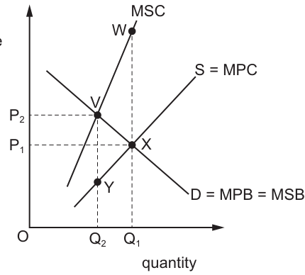
The diagram shows market failure caused by negative production externalities.
Identify the correct combination of the result of the market failure and the area on the diagram that shows deadweight welfare loss.
Options
| result of market failure | area showing deadweight welfare loss | |
|---|---|---|
| A | overproduction | VWX |
| B | overproduction | XYV |
| C | underproduction | VWX |
| D | underproduction | XYV |
Reasoning
A negative production externality means marginal social cost (MSC) is above marginal private cost (MPC), as producers do not bear the full external cost of production. The market equilibrium occurs where MPC = marginal private benefit (MPB, equal to MSB here) at point X, with quantity Q1. The socially optimal equilibrium occurs where MSC = MSB at point V, with quantity Q2. Since Q1 > Q2, the market overproduces relative to the social optimum. Deadweight welfare loss is the loss of social welfare from the overproduced units (Q2 to Q1), represented by the area between MSC and MSB over this quantity range, which is triangle VWX.
Answer
A
A
Background Concept
A negative production externality occurs when the production of a good or service imposes uncompensated costs on third parties not involved in the transaction. For example, a factory emitting pollution imposes health costs on nearby residents. In this case, the marginal private cost (MPC) faced by producers is lower than the marginal social cost (MSC), which includes both the private cost and the marginal external cost (MEC): MSC = MPC + MEC.
Market failure arises when the free market fails to allocate resources efficiently, leading to a deadweight welfare loss (DWL) — a loss of total social surplus that no one benefits from. For negative externalities, the market equilibrium (where private costs and benefits are balanced) differs from the socially optimal equilibrium (where all social costs and benefits are balanced).
Understanding the Question
This 1-mark multiple-choice question provides a standard diagram of a negative production externality and asks you to identify two things: (1) whether the market failure leads to overproduction or underproduction relative to the social optimum, and (2) which labelled area on the diagram represents the deadweight welfare loss. The diagram shows the demand curve (D = MPB = MSB, meaning private and social benefit are equal here, so no consumption externality), two supply curves (S = MPC and MSC, with MSC to the left of MPC, confirming a negative production externality), and four labelled points (V, W, X, Y) defining three potential triangular areas.
Approach
To answer this, follow two steps:
- Compare the market equilibrium quantity and the socially optimal quantity to determine if there is overproduction or underproduction.
- Identify the DWL area as the triangle representing the net social cost of the units produced beyond the social optimum, which lies between the MSC and MSB curves over the range of overproduced units.
Step-by-Step Reasoning
- First, identify the market equilibrium: this occurs where the private supply curve (MPC) intersects the private benefit curve (MPB, which equals MSB here). On the diagram, this is point X, at quantity Q1 and price P1.
- Next, identify the socially optimal equilibrium: this occurs where the social cost curve (MSC) intersects the social benefit curve (MSB). On the diagram, this is point V, at quantity Q2 and price P2.
- Compare the two quantities: Q1 (market quantity) is larger than Q2 (social optimum quantity). This means the free market produces more of the good than is socially desirable, so the result of the market failure is overproduction. This immediately eliminates options C and D, which state underproduction.
- Now identify the deadweight welfare loss: DWL is the value of the social welfare lost from the overproduced units (the units between Q2 and Q1). For each of these units, the marginal social cost (MSC) is higher than the marginal social benefit (MSB), so each unit creates a net social loss. The total DWL is the area between the MSC and MSB curves from Q2 to Q1.
- On the diagram, the MSC curve runs from point V (at Q2) up to point W (at Q1).
- The MSB (demand) curve runs from point V (at Q2) down to point X (at Q1).
- The area bounded by these two curves and the quantity difference between Q2 and Q1 is the triangle with vertices V, W, and X: area VWX.
- The alternative area XYV is the triangle between the MPC curve and the MSB curve over the same quantity range, which represents the private cost of the overproduced units, not the social welfare loss.
- The correct combination is overproduction and area VWX, which is option A.
Key Takeaways
- For negative production externalities, MSC > MPC, so the free market overproduces relative to the social optimum.
- Deadweight welfare loss from a negative production externality is the area between the MSC and MSB (demand) curves between the market quantity and the socially optimal quantity.
- Always distinguish between private costs/benefits and social costs/benefits when analysing externalities: DWL is based on social, not private, values.
Common Mistakes
- Confusing overproduction and underproduction: Negative production externalities lead to overproduction, because producers ignore external costs and produce too much. Underproduction is associated with positive externalities (e.g. education, vaccinations).
- Misidentifying the DWL area: Many students incorrectly select XYV, which is the area between MPC and MSB. This is not the DWL, because it only counts private costs, not the full social cost (MSC) that includes external costs. The DWL must include the external cost, so it lies between MSC and MSB.
- Forgetting that MSB = MPB here: Since there is no consumption externality, the demand curve represents both private and social benefit, so it is used to calculate the social optimum.
Things to Be Careful About
- Always check the direction of the MSC curve relative to MPC: if MSC is to the left of MPC (higher at every quantity), it is a negative production externality, leading to overproduction. If MSC is to the right, it is a positive production externality, leading to underproduction.
- When identifying DWL, always use the social cost and social benefit curves, not the private ones, as welfare loss is measured in terms of total social surplus.
- For 1-mark MCQs, you do not need to write an extended explanation, but you must be certain of the reasoning to avoid selecting a distractor.
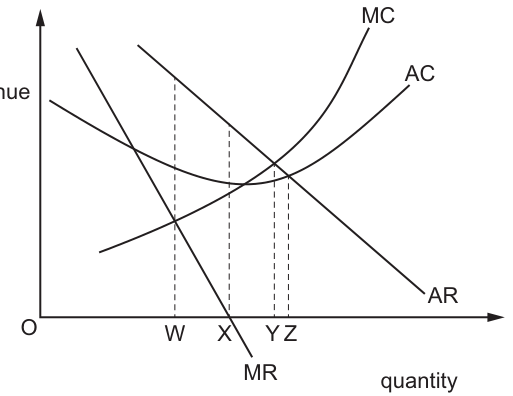
The diagram shows the cost and revenue curves of a firm.
The firm changes its objective from revenue maximisation to sales maximisation.
What will be the effect on quantity produced?
Options
A it will decrease from Y to W
B it will decrease from Z to W
C it will increase from X to Y
D it will increase from X to Z
Reasoning
Revenue maximisation occurs where marginal revenue (MR) equals zero, as this is the output level where total revenue is at its highest. On the diagram, MR intersects the horizontal quantity axis at output X, so the firm originally produces X.
Sales maximisation (subject to a normal profit constraint) occurs where average revenue (AR) equals average cost (AC), as this is the point where total revenue equals total cost (normal profit) and the firm can sell the maximum possible output without making a loss. On the diagram, AR intersects AC at output Z, so the new sales-maximising quantity is Z.
Quantity therefore increases from X to Z.
Answer
D
D
Background Concept
Firms may pursue a range of objectives beyond traditional profit maximisation, depending on their market context and priorities. Two common alternative objectives are revenue maximisation and sales maximisation.
Revenue maximisation is the goal of achieving the highest possible total revenue (TR, calculated as price × quantity sold). This occurs at the output level where marginal revenue (MR, the additional revenue from selling one more unit) equals zero. At outputs below this point, MR is positive, so selling more units increases total revenue; at outputs above this point, MR is negative, so selling more units reduces total revenue.
Sales maximisation, most associated with Baumol's model of firm behaviour, is the goal of selling the maximum possible quantity of output. Unlike revenue maximisation, sales maximisation is subject to a minimum profit constraint: the firm must at least cover its total costs to remain viable in the long run. The minimum acceptable profit is normal profit (zero economic profit), which occurs where total revenue equals total cost. Since average revenue (AR, total revenue per unit) equals average cost (AC, total cost per unit) when TR = TC, sales maximisation occurs at the output where AR = AC.
The diagram provided shows standard cost and revenue curves for a price-setting firm (facing a downward-sloping demand curve): AR is the average revenue (demand) curve, MR is the marginal revenue curve (below AR because the firm must lower price for all units to sell more), AC is the U-shaped average cost curve, and MC is the U-shaped marginal cost curve.
Understanding the Question
The question presents a cost and revenue diagram for a firm, and states that the firm changes its objective from revenue maximisation to sales maximisation. It asks what the effect on the quantity produced will be, with four options describing different changes in output. This is a 1-mark multiple-choice question that tests knowledge of two alternative firm objectives, their corresponding output rules, and the ability to apply these rules to a labelled diagram. The core task is to match each objective to its correct equilibrium output on the diagram, then identify the direction and magnitude of the change in quantity.
Approach
To solve this question, follow two steps:
- First, recall the unique output condition for each of the two objectives:
- Revenue maximisation: MR = 0 (total revenue is maximised here)
- Sales maximisation (with normal profit constraint): AR = AC (TR = TC, normal profit is earned)
- Second, locate these conditions on the provided diagram using the labelled quantity points (W, X, Y, Z) to find the original and new output levels, then compare them to determine the change.
Step-by-Step Reasoning
- Identify the revenue-maximising output: Total revenue is the total amount of money a firm earns from selling its output. Marginal revenue is the change in total revenue from selling one additional unit. When MR is positive, increasing output raises total revenue; when MR is negative, increasing output lowers total revenue. The maximum total revenue is therefore reached at the output where MR = 0, as this is the final unit that adds to total revenue. On the diagram, the MR curve slopes downward and intersects the horizontal quantity axis at output X, meaning MR = 0 at X. This is the firm's original revenue-maximising quantity.
- Identify the sales-maximising output: Sales maximisation requires the firm to sell as much as possible while still covering its costs to avoid losses. The minimum acceptable level of profit is normal profit, where the firm makes zero economic profit (it covers all its costs, including opportunity costs). Normal profit occurs where total revenue equals total cost. Since AR = TR / Q and AC = TC / Q, TR = TC is equivalent to AR = AC. On the diagram, the AR curve intersects the AC curve at output Z, meaning AR = AC at Z. This is the highest output the firm can produce while still earning normal profit, so it is the sales-maximising quantity.
- Compare the two quantities: The original revenue-maximising quantity is X, and the new sales-maximising quantity is Z. Since Z is to the right of X on the quantity axis (higher quantity), the quantity produced increases from X to Z.
- Match to the options: Option D states "it will increase from X to Z", which matches our conclusion.
Key Takeaways
- Always link each firm objective to its specific equilibrium condition: profit maximisation uses MC = MR, revenue maximisation uses MR = 0, and sales maximisation (with normal profit constraint) uses AR = AC.
- When analysing diagrams, first identify what each intersection of curves represents before matching it to the question's requirements.
- Sales maximisation is not the same as revenue maximisation: revenue maximisation focuses on the highest total revenue regardless of profit, while sales maximisation focuses on the highest quantity sold, subject to making at least normal profit.
Common Mistakes
- Confusing the output conditions for different objectives: A common error is to assume sales maximisation also uses MR = 0, but the two objectives have distinct rules. Another error is to use the profit-maximising condition (MC = MR, output W) for either objective, which is incorrect.
- Misreading the diagram: Failing to correctly identify which curve intersection corresponds to which output rule, for example mixing up the output where MR = 0 (X) with the output where AR = AC (Z).
- Misunderstanding the sales maximisation constraint: Some students incorrectly assume sales maximisation means producing the highest possible output regardless of profit, but the normal profit constraint means the firm stops at AR = AC, not at the maximum capacity output.
- Forgetting that revenue maximisation can involve losses: The revenue-maximising output (X) may be where the firm makes a loss if AC is above AR at that output, but this does not affect the output rule for revenue maximisation.
Things to Be Careful About
- Always verify which curve is which on the diagram: MR is the steeper downward-sloping curve below AR, AC is the U-shaped curve, MC is the upward-sloping curve that intersects AC at its minimum.
- Confirm the direction of the change: The question asks for the effect on quantity produced, so focus on whether quantity increases or decreases, not on price or profit changes.
- Remember that the sales maximisation point is where AR = AC, not where MC = MR or MR = 0: these are the conditions for other objectives, so mixing them up will lead to the wrong answer.
The diagrams show the demand curve, D1, and the supply curve, S1, for a good that has a sales tax of 10% applied to the final selling price.
Which diagram shows the impact of a reduction in the rate of sales tax to 5%?
Options
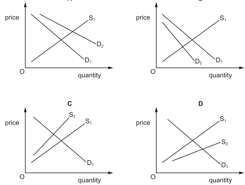
Working
A sales tax is an indirect tax levied on the sale of a good, which increases the cost of supplying each unit. This means a change in the sales tax rate affects the supply curve, not the demand curve, so options A and B (which show demand curve shifts) can be eliminated immediately.
A reduction in the sales tax rate from 10% to 5% lowers the cost of supplying the good. This makes firms willing to supply more at every price level, so the supply curve shifts to the right (outwards) from the original supply curve S1.
Option C shows a shift from S2 to S1, which would mean the supply curve moves to the original S1, which is incorrect as S1 is the starting point. Option D shows a rightward shift from S1 to S2, which matches the effect of a lower sales tax.
Answer
D
D
Background Concept
A sales tax is a type of indirect tax, charged as a percentage of the final selling price of a good (in this case, an ad valorem tax of 10% initially, then 5%). Indirect taxes are imposed on the production or sale of a good, rather than directly on consumers' income. For suppliers, the sales tax increases the cost of selling each unit: the revenue a firm receives from a sale is the price paid by the consumer minus the tax owed to the government. As a result, the supply curve (which plots the minimum price firms require to supply each quantity) shifts left (or upwards) when a sales tax is introduced or increased, and shifts right (or downwards) when the sales tax is reduced.
It is important to distinguish between factors that shift the demand curve and factors that shift the supply curve. The demand curve shifts only when there is a change in non-price determinants of demand, such as consumer income, tastes, or the price of related goods. A sales tax does not directly change these factors: while it may raise the price consumers pay, this causes a movement along the existing demand curve, not a shift of the curve itself.
Understanding the Question
The question presents four supply and demand diagrams for a market with initial curves D1 (demand) and S1 (supply), where a 10% sales tax is already applied. The task is to identify which diagram correctly shows the effect of reducing this sales tax to 5%. The four options are:
- A: Demand shifts right from D1 to D2, supply unchanged
- B: Demand shifts left from D1 to D2, supply unchanged
- C: Supply shifts right from S2 to S1, demand unchanged
- D: Supply shifts right from S1 to S2, demand unchanged
The question tests understanding of how changes in indirect tax rates affect market curves, and the ability to interpret the direction and starting point of curve shifts in a diagram.
Approach
To solve this, follow two steps:
- First, identify which curve is affected by a sales tax: since sales tax is a tax on the sale of the good, it impacts the supply side, not demand. This immediately eliminates options A and B, which show demand curve shifts.
- Second, determine the direction of the supply shift: a lower sales tax reduces the cost of supplying each unit, so firms will supply more at every price. This means the supply curve shifts to the right (outwards, away from the price axis). We then match this to the remaining options, checking that the shift starts at the original supply curve S1.
Step-by-Step Reasoning
- Eliminate demand-shift options: A sales tax is not a change in consumer preferences, income, or the price of substitutes/complements, so it does not alter the underlying demand for the good. The only effect on demand is a change in the price consumers pay, which is a movement along the demand curve, not a shift. Options A and B both show the demand curve shifting, so they are incorrect.
- Determine the direction of the supply shift: The original supply curve S1 already includes the 10% sales tax in its position. When the tax rate falls to 5%, the tax per unit of output decreases. For any given quantity, the total price consumers pay (including tax) will be lower than before, or equivalently, the price producers receive for a given consumer price will be higher. This lower cost of supply means firms are willing to sell more at every price level, so the supply curve shifts to the right (outwards).
- Match to the correct diagram:
- Option C shows the supply curve shifting from S2 (left of S1) to S1 (the original curve). This would represent an increase in supply, but the shift originates at S2, not the original S1, so it does not match the scenario where we start at S1 and reduce the tax.
- Option D shows the supply curve shifting from S1 (the original curve with 10% tax) to S2 (to the right of S1). This is a rightward shift in supply, exactly matching the effect of a lower sales tax.
- Conclusion: Diagram D is the correct representation.
Key Takeaways
- Indirect taxes (sales tax, excise duties) shift the supply curve, not the demand curve.
- A reduction in an indirect tax shifts the supply curve to the right (increase in supply); an increase shifts it to the left (decrease in supply).
- When interpreting curve shift diagrams, always confirm that the shift starts at the original curve labelled in the question.
Common Mistakes
- Shifting the demand curve: Many students incorrectly assume that a tax on a good affects demand, but sales tax is a supply-side cost. Only changes in non-price demand determinants shift the demand curve.
- Wrong shift direction: Some students mistakenly think a tax cut reduces supply, but lower costs increase the quantity firms are willing to supply at each price, so supply shifts right.
- Misidentifying the original curve: Option C shows a shift ending at S1, but S1 is the original supply curve, so the shift must start at S1. This is a common error when students do not check the direction of the arrow or the labels of the curves.
Things to Be Careful About
- Always distinguish between factors that shift curves versus factors that cause movements along curves: a sales tax changes the cost of supply, so it shifts the supply curve; it does not shift demand.
- Check the direction of the shift relative to the original curve: the question states the original supply is S1, so the shift must be from S1, not to S1.
- Remember that ad valorem (percentage) taxes have the same directional effect on supply as specific (per-unit) taxes: a lower tax rate always increases supply, shifting the curve right.
Which government policy is intended to correct a negative externality?
Options
A guaranteed minimum prices for farmers producing certain agricultural products
B imposition of taxes on factories releasing pollutants into rivers
C rent controls on housing occupied by low-income individuals
D the provision of free books for children of poorer households
Answer
A negative externality occurs when a third party bears a cost from a transaction in which they are not involved. The government can internalise this external cost by imposing a tax equal to the marginal external cost. Option B — a tax on factories releasing pollutants — is the textbook example of such a Pigouvian tax, designed to correct the negative externality of pollution.
Answer
B
B
Background Concept
A negative externality is a cost imposed on a third party who is not directly involved in a market transaction. For example, when a factory releases pollutants into a river, the factory and its customers benefit from production, but people downstream suffer from polluted water — a cost not reflected in the market price. This leads to overproduction relative to the socially optimal level, because the private cost (borne by the factory) is less than the social cost (private cost + external cost).
Governments can correct this market failure by internalising the externality — making the polluter pay the full social cost. The standard policy is a Pigouvian tax (named after economist Arthur Pigou), set equal to the marginal external cost at the socially efficient output. This shifts the supply curve upward (or leftward), reducing output to the socially optimal level.
Understanding the Question
This is a multiple-choice question asking which of four government policies is intended to correct a negative externality. The key word is "intended" — the policy's purpose must be to address an external cost, not to achieve some other goal (like income redistribution or price stabilisation). You need to recognise each option's primary economic rationale and match it to the type of market failure it targets.
Approach
For each option, ask: "What market failure is this policy designed to fix?"
- Option A: guaranteed minimum prices for farmers — this is a price support policy, typically aimed at stabilising farm incomes or ensuring food security, not correcting an externality.
- Option B: taxes on factories releasing pollutants — this directly targets the negative externality of pollution by making the polluter pay.
- Option C: rent controls on housing for low-income individuals — this is a price control intended to make housing more affordable, a redistribution or equity policy, not an externality correction.
- Option D: free books for children of poorer households — this addresses equity and possibly a positive externality (education benefits society), but it is not correcting a negative externality.
Only option B fits the definition of a corrective measure for a negative externality.
Step-by-Step Reasoning
- Define negative externality: A cost borne by a third party not involved in the transaction. Pollution is the classic example.
- Identify the policy's purpose: A tax on polluters raises the private cost of production to match the social cost, reducing output to the socially efficient level. This is a Pigouvian tax.
- Check each option:
- A: Minimum prices for farmers — this is a price floor, often used to support farm incomes or stabilise agricultural markets. It does not target an external cost; it may even create a surplus (a different type of inefficiency).
- B: Tax on polluting factories — directly addresses the negative externality. Correct.
- C: Rent controls — a price ceiling intended to make housing affordable for low-income tenants. It addresses equity, not an externality. It may even create a shortage (inefficiency).
- D: Free books for poor children — this is a subsidy or direct provision aimed at improving educational outcomes and reducing inequality. It might address a positive externality (educated population benefits society), but it is not correcting a negative externality.
- Conclusion: Only option B is a policy intended to correct a negative externality.
Key Takeaways
- A negative externality leads to overproduction because private costs are less than social costs.
- The standard corrective policy is a Pigouvian tax (or a pollution permit system) that internalises the external cost.
- Not all government interventions are about externalities — many address equity, stabilisation, or other objectives.
- When answering multiple-choice questions on market failure, match the policy to the specific type of failure described.
Common Mistakes
- Confusing a negative externality with a positive one. Option D (free books) might be thought to correct a negative externality, but it actually addresses a positive externality (education benefits society) or equity.
- Thinking that any government intervention in a market is about correcting an externality. Rent controls and minimum prices are about other goals (affordability, income support).
- Not reading the question carefully: the word "intended" is crucial — the policy's purpose, not its side effects, determines the answer.
Things to Be Careful About
- Remember the definition: a negative externality imposes a cost on third parties. Pollution is the classic example, but others include noise, congestion, and second-hand smoke.
- A tax on a negative externality is called a Pigouvian tax. It is set equal to the marginal external cost.
- In multiple-choice questions, eliminate options that clearly address other objectives (equity, stabilisation, income support) before choosing the one that targets the externality directly.
Which policy is most likely to contribute to people ending up in a poverty trap?
Options
A legal minimum wage
B means-tested benefits
C prevention of cheaper imports
D proportional taxation
Answer
A poverty trap occurs when an individual's net income does not rise (or rises very little) when they increase their gross earned income, because means-tested benefits are withdrawn as earnings rise. This creates a disincentive to work more or seek higher pay. Option B, means-tested benefits, is therefore the policy most likely to contribute to a poverty trap.
B
Background Concept
The poverty trap (also called the unemployment trap or the welfare trap) is a situation where an individual or household has little or no net financial gain from increasing their earned income. This happens because as gross earnings rise, means-tested benefits (such as housing benefit, income support, or tax credits) are withdrawn, and income tax and National Insurance contributions may also increase. The combined effect can mean that disposable income rises by only a small amount, or even falls, for each additional pound earned. This creates a disincentive to work more hours, seek promotion, or move from welfare into paid employment.
Means-tested benefits are payments that depend on the recipient's income and/or assets. They are designed to target support to those with the lowest incomes. However, the withdrawal of these benefits as income rises creates a high effective marginal tax rate, which is the core mechanism of the poverty trap.
Understanding the Question
This is a multiple-choice question asking which of four policies is most likely to contribute to people ending up in a poverty trap. The key is to understand the mechanism that creates the trap: a reduction in net income gain when gross income rises. The correct answer is the policy that directly creates this disincentive effect.
Approach
Evaluate each option in turn, considering whether it creates a disincentive to increase income. The correct answer is the one that does so most directly and strongly.
Step-by-Step Reasoning
-
Option A: Legal minimum wage. A minimum wage raises the hourly pay of low-paid workers. This increases their gross income, which reduces the likelihood of being in a poverty trap (it makes work more rewarding). It does not create a withdrawal of benefits. So A is incorrect.
-
Option B: Means-tested benefits. These are explicitly withdrawn as income rises. For example, if a person earns an extra £10, they may lose £8 of housing benefit, leaving a net gain of only £2. This high effective marginal tax rate (the 'taper rate') is the classic cause of the poverty trap. Therefore B is correct.
-
Option C: Prevention of cheaper imports. This is a protectionist trade policy. It may raise the price of imported goods, reducing the real purchasing power of low-income households, but it does not directly create a disincentive to increase earned income. It is not a cause of the poverty trap. So C is incorrect.
-
Option D: Proportional taxation. A proportional tax (flat tax) takes the same percentage of income at all income levels. While it does reduce net income, it does not create a high marginal rate at low incomes (unlike means-test withdrawal). It does not, by itself, create a poverty trap. So D is incorrect.
Key Takeaways
- The poverty trap is caused by the withdrawal of means-tested benefits as income rises, creating a high effective marginal tax rate.
- Means-tested benefits are the policy most directly associated with this trap.
- Policies that increase the reward for working (like a minimum wage) or that do not create a withdrawal mechanism (like universal benefits or proportional taxes) do not cause a poverty trap.
Common Mistakes
- Confusing the poverty trap with low income itself. The trap is about the disincentive to increase income, not simply being poor.
- Thinking that any tax or benefit that reduces net income creates a poverty trap. The key is the withdrawal rate at the margin, not the average level of support.
- Choosing 'prevention of cheaper imports' because it might harm the poor, but failing to see it does not create a work disincentive.
Things to Be Careful About
- The question asks for the policy most likely to contribute to the trap. Means-tested benefits are the textbook cause.
- Understand the difference between means-tested and universal benefits. Universal benefits (e.g., child benefit) are not withdrawn as income rises and do not create a poverty trap.
- The poverty trap is a supply-side issue: it reduces the incentive to supply labour. It is a form of market failure in the labour market caused by government policy.
Extra fishing boats start to operate from a local harbour which depends on fishing for its main income.
Which action by the local authority is an example of nudge theory?
Options
A insisting that all fish caught are sold to local people
B increasing the licence fees for new boats
C distributing leaflets about the need to safeguard fish stocks
D restricting the areas in which boats can fish
Reasoning
Nudge theory involves changing people's behaviour in a predictable way without forbidding any options or significantly changing their economic incentives. Option C — distributing leaflets about the need to safeguard fish stocks — provides information to influence behaviour voluntarily, without coercion or a financial penalty. Options A and D are direct regulations (insisting and restricting), and option B uses a price mechanism (higher licence fees) to discourage entry. Only C fits the definition of a nudge.
Answer
C
C
Background Concept
Nudge theory, developed by Thaler and Sunstein, is a concept in behavioural economics. It suggests that positive reinforcement and indirect suggestions can influence the behaviour and decision-making of groups or individuals. A 'nudge' alters the environment, or 'choice architecture', in a way that makes it more likely that people will make a particular choice, but without removing their freedom of choice or significantly altering their economic incentives. Classic examples include placing healthier food at eye level in a cafeteria, or automatically enrolling employees into a pension scheme while allowing them to opt out. The key is that it is not a mandate, a ban, or a significant financial penalty/reward.
Understanding the Question
This is a multiple-choice question testing the understanding of 'nudge theory' as a specific government policy tool to correct market failure. The scenario is a local harbour where extra fishing boats are starting to operate, threatening fish stocks (a common pool resource problem). The question asks which of the four actions by the local authority is an example of nudge theory. The candidate must distinguish a nudge from other policy tools: direct regulation (quotas, bans), market-based instruments (taxes, subsidies, tradable permits), and direct provision of information. The correct answer is the one that influences behaviour through information and choice architecture without coercion or significant financial cost.
Approach
- Recall the precise definition of nudge theory: a change in choice architecture that alters behaviour predictably without forbidding any options or significantly changing economic incentives.
- Evaluate each option against this definition:
- A (insisting): This is a direct command or regulation, removing the freedom to sell elsewhere. Not a nudge.
- B (increasing licence fees): This is a financial disincentive (a tax-like measure), significantly changing the economic incentive. Not a nudge.
- C (distributing leaflets): This provides information. It does not force anyone to act, nor does it change the cost of fishing. It relies on voluntary behaviour change after receiving information. This fits the definition of a nudge.
- D (restricting areas): This is a direct regulation (a quota on where to fish), removing the freedom to fish in certain areas. Not a nudge.
- Select the option that best matches the definition.
Step-by-Step Reasoning
- Identify the core problem: Overfishing in a local harbour. This is a negative externality (or a tragedy of the commons) where individual boat owners have an incentive to catch as many fish as possible, leading to depletion of the stock for everyone.
- Define the policy tool: Nudge theory. The defining characteristic is that it steers people's choices without coercion or significant financial penalty. It works by changing the context in which decisions are made.
- Analyse Option A: 'Insisting that all fish caught are sold to local people'. This is a command. It removes the fishermen's freedom to choose where to sell. This is a form of direct regulation, not a nudge.
- Analyse Option B: 'Increasing the licence fees for new boats'. This is a price-based intervention. It makes it more expensive to enter the fishing industry, thereby reducing the number of boats. This significantly changes the economic incentive (the cost of entry). This is a market-based policy, not a nudge.
- Analyse Option C: 'Distributing leaflets about the need to safeguard fish stocks'. This is an information campaign. It provides information to fishermen about the consequences of overfishing. It does not force them to fish less, nor does it make it more expensive to fish. It relies on the fishermen voluntarily changing their behaviour after being informed. This is a classic example of a nudge.
- Analyse Option D: 'Restricting the areas in which boats can fish'. This is a direct regulation (a spatial quota). It removes the freedom to fish in certain areas. This is a command-and-control policy, not a nudge.
- Conclusion: Only Option C fits the definition of a nudge.
Key Takeaways
- Nudge theory is a distinct policy approach that relies on changing choice architecture, not on coercion or significant financial incentives.
- The key differentiators are: (1) freedom of choice is preserved, (2) economic incentives are not significantly altered, and (3) the intervention works by influencing the decision-making context.
- Common examples of nudges include: default options, information campaigns, social norm messaging, and changes to the physical environment (e.g., placing stairs more prominently than escalators).
- Be able to distinguish nudges from: taxes/subsidies, regulations/bans, and direct provision of services.
Common Mistakes
- Confusing information provision with regulation: A student might think that providing information is a form of regulation. It is not, unless the information is mandatory and enforced. A leaflet is a suggestion, not a rule.
- Confusing a nudge with a financial incentive: A student might think that a licence fee is a 'nudge' because it is not a complete ban. However, a significant financial cost is a market-based incentive, not a nudge. A nudge would be something like automatically enrolling boats in a sustainable fishing program with an opt-out, rather than charging them to enter.
- Overthinking: A student might try to find a 'behavioural' element in all options. The key is to apply the strict definition. 'Insisting' and 'restricting' are clearly not nudges.
Things to Be Careful About
- Read the definition carefully: The question is testing the specific definition of nudge theory from the syllabus. Do not rely on a general, vague understanding of the word 'nudge'.
- Focus on the mechanism: Ask yourself: does this policy work by (a) forcing, (b) pricing, or (c) informing and influencing? Only (c) is a nudge.
- Consider the 'freedom of choice' criterion: A nudge must preserve freedom of choice. Options A and D remove choice. Option B makes a choice more expensive but does not remove it, but the cost is a significant economic change. Option C preserves full freedom and only provides information.
The diagram shows the effect of introducing an effective national minimum wage (NMW) in a labour market with a profit maximising monopsonist employer.
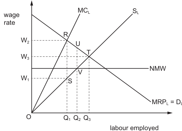
What is the effect of the NMW on the deadweight welfare loss in this market?
Options
A It falls from RST to UVT.
B It falls from RSVU to UVT.
C It rises from UVT to RST.
D It rises from UVT to RSVU.
Reasoning
A profit-maximising monopsonist hires labour where the marginal cost of labour (MCL) equals the marginal revenue product of labour (MRPL = DL). On the diagram, this intersection is at point R, so original employment is Q1, and the wage paid is given by the supply of labour (SL) at Q1, which is W1 (point S). The deadweight welfare loss (DWL) from monopsony power is the area of mutually beneficial trades that do not occur between Q1 and the perfectly competitive employment level (where SL = MRPL at point T, Q3). This area is the triangle RST.
When an effective national minimum wage (NMW) is introduced at W2, the firm’s marginal cost of labour becomes constant at W2 up to the quantity where SL meets the NMW (point V, Q2). The firm now hires where the NMW equals MRPL, which is point U, giving a new employment level of Q2 (higher than Q1). The new DWL is the area of missed trades between Q2 and Q3, which is the triangle UVT.
Comparing the two areas, the DWL falls from RST to UVT.
Answer
A
A
Background Concept
A monopsonist is a market structure where there is only one (or a dominant) buyer of a good or service — in this case, labour. Unlike a perfectly competitive labour market where individual firms are wage-takers, a monopsonist has market power as a buyer, allowing it to set wages below the competitive level by restricting the quantity of labour it hires.
Key curves in the monopsony labour market diagram:
- SL (supply of labour): upward-sloping, shows the wage required to attract each additional worker. This is the average cost of labour to the firm.
- MCL (marginal cost of labour): upward-sloping and steeper than SL, because to hire an extra worker, the monopsonist must raise the wage for all existing workers, so the marginal cost of each additional worker is higher than the wage paid to that worker.
- MRPL = DL (marginal revenue product of labour / demand for labour): downward-sloping, shows the additional revenue the firm earns from hiring one more worker. It slopes down due to the law of diminishing marginal returns: as more workers are hired, each additional worker adds less to output and revenue.
Deadweight welfare loss (DWL) in this context is the loss of total economic surplus (the sum of worker surplus and firm surplus) that arises because the monopsonist employs fewer workers than the socially optimal level. For workers between the monopsony employment level and the competitive level, the MRPL (the value of their output to the firm) is higher than the wage they would accept (given by SL), so these are mutually beneficial trades that do not happen under monopsony, creating a welfare loss.
A national minimum wage (NMW) is a legally enforced wage floor set above the equilibrium wage. In a monopsony market, a NMW set above the monopsonist’s original wage but below the competitive wage can increase both wages and employment: it forces the monopsonist to pay a higher wage, removing its incentive to restrict hiring to keep wages low.
Understanding the Question
The question provides a labelled diagram of a labour market with a profit-maximising monopsonist employer, and shows the introduction of an effective NMW (a wage floor that is binding, i.e., above the original market wage). It asks what happens to the deadweight welfare loss in this market as a result of the NMW. The four options describe different changes to the DWL area, identified by the labelled points R, S, T, U, V on the diagram.
The question tests two core sets of knowledge: (1) how a monopsonist determines its employment and wage level, and how a NMW affects this; (2) how to identify the DWL area on a labour market diagram, and how it changes when a policy alters the employment level. The correct answer requires matching the pre- and post-NMW DWL areas to the options.
Approach
To solve this question, follow these steps:
- First, identify the original monopsony equilibrium without the NMW: find the quantity where MCL = MRPL (the firm’s profit-maximising rule), and the corresponding wage from the SL curve.
- Identify the original DWL: this is the area between the MRPL (marginal benefit of labour) and SL (marginal cost of labour) for all units between the monopsony employment level and the perfectly competitive employment level (where SL = MRPL).
- Next, identify the new equilibrium with the NMW: the NMW is a horizontal line, so the firm’s MCL becomes constant at the NMW level up to the point where SL intersects the NMW. The firm hires where the NMW equals MRPL.
- Identify the new DWL: the area between MRPL and SL between the new employment level and the competitive level.
- Compare the two DWL areas to see if they rise or fall, and match to the given options.
Step-by-Step Reasoning
Let’s apply this approach to the diagram:
- Original monopsony equilibrium: The monopsonist maximises profit by hiring where MCL = MRPL. On the diagram, MCL and MRPL intersect at point R, so the original employment level is Q1. The wage the monopsonist pays is determined by the SL curve at Q1: this is point S, so the original wage is W1.
- Perfectly competitive equilibrium: If there were many employers competing for workers, the equilibrium would be where SL (labour supply) equals MRPL (labour demand). This occurs at point T, with employment Q3 and wage W3. This is the socially optimal level of employment, as all mutually beneficial trades (where MRPL > SL) occur here.
- Original DWL: The DWL from monopsony power is the value of the missed mutually beneficial trades between Q1 and Q3. This is the triangular area bounded by the MRPL curve above, the SL curve below, and the vertical line at Q1. The vertices of this triangle are R (Q1, W2), S (Q1, W1), and T (Q3, W3), so the original DWL is area RST.
- Effect of the NMW: The NMW is set at W2 (the horizontal line on the diagram), which is above the original monopsony wage W1. For the monopsonist, the marginal cost of hiring workers up to the point where SL meets the NMW is now constant at W2, because the firm can hire any number of workers up to Q2 at the fixed wage W2. The firm will hire up to the point where the NMW equals the MRPL, because beyond this point, the MRPL is lower than the cost of hiring a worker. This intersection is at point U, so the new employment level is Q2 (higher than the original Q1).
- New DWL: The missed trades now only occur between Q2 and Q3, as employment has increased. The new DWL is the triangular area bounded by MRPL above, SL below, and the vertical line at Q2. The vertices of this triangle are U (Q2, W2), V (Q2, W1), and T (Q3, W3), so the new DWL is area UVT.
- Comparison and elimination of wrong options: The original DWL (RST) is larger than the new DWL (UVT), because Q2 is closer to the competitive quantity Q3 than Q1 is, so fewer mutually beneficial trades are missed. This means DWL falls from RST to UVT, which matches option A.
- Option B is incorrect because it misidentifies the original DWL as RSVU, a quadrilateral that includes the area between MCL and SL. DWL only measures the gap between the marginal benefit of labour (MRPL) and the marginal cost of labour (SL), so the area between MCL and SL is not part of DWL.
- Options C and D are incorrect because they state DWL rises, which would only happen if the NMW reduced employment below Q1. In this case, the NMW increases employment to Q2, so DWL falls.
Key Takeaways
- A monopsonist restricts employment below the perfectly competitive level to reduce wages, creating a DWL from un-hired workers who would have generated more revenue for the firm than the wage they require.
- A national minimum wage set above the monopsonist’s wage but below the competitive wage increases both wages and employment in a monopsony market, by eliminating the monopsonist’s incentive to restrict hiring. This reduces the DWL by moving employment closer to the socially optimal level.
- When identifying DWL on a labour market diagram, always use the demand for labour (MRPL) and supply of labour (SL) curves, not the MCL curve, as DWL is based on the marginal benefit and marginal cost of labour to society, not the firm’s private marginal cost.
- Always check the direction of the change in employment when evaluating the impact of a NMW: in monopsony, a binding NMW increases employment, while in perfect competition it reduces employment.
Common Mistakes
- Using the wrong employment rule for monopsony: Many students incorrectly assume a monopsonist hires where SL = MRPL (the competitive rule). The correct rule is MCL = MRPL, which gives a lower employment level (Q1) than the competitive level (Q3). Using the wrong rule leads to misidentifying the original employment level and thus the DWL area.
- Misidentifying the DWL area: Some students include the area between MCL and SL in the DWL, but this area represents the monopsonist’s economic rent (the difference between the marginal cost of labour and the wage paid), not a welfare loss. DWL only includes the area between MRPL and SL for un-hired workers.
- Assuming NMW always reduces employment: This is true for perfectly competitive labour markets, but not for monopsony. In monopsony, a NMW set at or below the competitive wage increases employment, so DWL falls. Applying the perfect competition result to monopsony leads to selecting the wrong option.
- Misreading the diagram’s point labels: Confusing the positions of points R, U, S, V can lead to selecting the wrong area. For example, mixing up R (original MCL=MRPL point) and U (new NMW=MRPL point) would lead to identifying the wrong DWL area.
Things to Be Careful About
- Always confirm the type of labour market: this question is about a monopsony, not perfect competition, so the standard perfect competition analysis of NMW (reducing employment) does not apply.
- When identifying DWL, use the MRPL (demand) and SL (supply) curves, not the MCL curve. The MCL is the firm’s private cost, but the social cost of hiring a worker is the wage they require (given by SL).
- Match the area labels exactly to the points in the options: the original DWL is the triangle with vertices R, S, T; the new DWL is the triangle with vertices U, V, T. Do not confuse these with other areas on the diagram.
- Verify the direction of change: since employment rises from Q1 to Q2, the DWL (the area between the employment level and Q3) must shrink, so the correct option must state that DWL falls. This immediately eliminates options C and D, which state DWL rises.
What is an advantage of pollution permits, when compared with an alternative policy of taxes levied on the quantity of pollutants emitted by firms?
Options
A firms cannot sell any surplus permits
B no monitoring of firms’ emissions is required
C pollution levels can be reduced to zero
D the reduction in the level of pollution is more predictable
Answer
Pollution permits set a fixed total quantity of allowable emissions, so the government directly controls the maximum pollution level. In contrast, a tax on emissions fixes the price of polluting but leaves the final quantity of emissions uncertain, because firms' responses depend on their marginal abatement costs. Therefore, the reduction in pollution is more predictable under a permit system.
Answer
D
D
Background Concept
Both pollution permits and pollution taxes are market-based instruments designed to correct the market failure caused by negative externalities, such as pollution. The key difference lies in what the government controls directly:
- Pollution permits (cap-and-trade): The government sets a maximum total quantity of pollution (the cap) and issues permits equal to that cap. Firms must hold permits for each unit of pollution they emit. The price of permits is determined by the market (supply and demand). The government controls the quantity of pollution.
- Pollution taxes (Pigouvian tax): The government sets a tax per unit of pollution emitted. Firms will reduce pollution as long as the cost of doing so (marginal abatement cost) is less than the tax. The government controls the price of pollution. The final quantity of pollution depends on how much firms choose to abate, which is uncertain if the government does not know firms' abatement costs perfectly.
Understanding the Question
The question asks for an advantage of pollution permits compared to a tax on emissions. It is a direct comparison. The correct answer must be something that permits do better than taxes. The options present four claims; we need to identify which one is a genuine advantage of permits.
Approach
Evaluate each option against the core difference between permits and taxes:
- Option A: 'firms cannot sell any surplus permits' – This is false. A key feature of a permit system is that permits are tradeable. Firms that reduce pollution cheaply can sell their surplus permits to firms for whom abatement is expensive. This is a major advantage (cost-effectiveness).
- Option B: 'no monitoring of firms’ emissions is required' – This is false. Both systems require monitoring to ensure firms comply. A permit system requires monitoring to check that firms' emissions do not exceed the permits they hold. A tax requires monitoring to calculate the tax bill.
- Option C: 'pollution levels can be reduced to zero' – This is false. The government can set the cap at zero, but this is not an inherent advantage of permits over taxes. A government could also set a tax so high that it drives pollution to zero. Both can theoretically achieve zero, but neither has a unique advantage here. In practice, setting the cap to zero would be extremely disruptive.
- Option D: 'the reduction in the level of pollution is more predictable' – This is true. Under a permit system, the government sets the maximum quantity of pollution directly. The outcome in terms of total pollution is certain (assuming perfect enforcement). Under a tax, the final quantity of pollution is uncertain because it depends on firms' unknown abatement costs. This is the classic argument for quantity-based instruments over price-based instruments when the marginal social cost of pollution is steep.
Step-by-Step Reasoning
- Identify the core difference: Permits control quantity; taxes control price.
- Analyze Option A: The statement is factually incorrect. The ability to trade permits is a key advantage, not a disadvantage. This option describes a disadvantage that does not exist.
- Analyze Option B: Both policies require monitoring. A tax requires monitoring to assess the tax; permits require monitoring to ensure compliance with the cap. Neither avoids monitoring.
- Analyze Option C: While a government could set a cap of zero, this is not a practical or inherent advantage. A tax could also be set high enough to achieve zero pollution. The question asks for an advantage of permits when compared to taxes. Both can theoretically achieve zero, so this is not a distinguishing advantage.
- Analyze Option D: This is the correct answer. Under a permit system, the total quantity of pollution is fixed by the cap. The government knows exactly the maximum amount of pollution that will be emitted. Under a tax, the government sets the price, but the resulting quantity depends on firms' responses. If the government has imperfect information about firms' abatement costs, the quantity outcome is uncertain. Therefore, permits offer greater predictability regarding the level of pollution reduction.
Key Takeaways
- The fundamental distinction between price-based (taxes, subsidies) and quantity-based (permits, quotas) regulatory instruments.
- Pollution permits provide certainty about the environmental outcome (quantity), while taxes provide certainty about the cost to firms (price).
- The choice between them depends on which uncertainty is more damaging: uncertainty about the quantity of pollution or uncertainty about the cost of abatement.
- Tradeability is a key feature of permit systems, allowing for cost-effective reductions.
Common Mistakes
- Confusing the direction of control: Thinking that a tax controls quantity or that a permit controls price. This leads to selecting the wrong option.
- Assuming permits eliminate the need for monitoring: Both systems require enforcement and monitoring.
- Thinking permits can always reduce pollution to zero: While theoretically possible, this is not a practical advantage and is not unique to permits.
- Not reading the question carefully: The question asks for an advantage of permits compared to taxes. Option A describes a disadvantage that is not even true of permits.
Things to Be Careful About
- Focus on the comparative advantage. The question is not asking about the merits of permits in isolation, but how they are better than taxes in a specific way.
- Remember the key feature of tradeability in a permit system. This is a major advantage that is often tested.
- Understand the information problem: the government's lack of knowledge about firms' abatement costs is the reason why the quantity outcome under a tax is uncertain.
Which statement about the quantity theory of money is correct?
Options
A It suggests changes in liquidity preference lead to proportional changes in the price level.
B It suggests changes in the money supply lead to proportional changes in the price level.
C It suggests changes in the price level lead to proportional changes in liquidity preference.
D It suggests changes in the price level lead to proportional changes in the money supply.
Answer
The quantity theory of money is expressed as MV = PT. Assuming V (velocity of circulation) and T (volume of transactions) are constant in the short run, a change in M (money supply) leads to a proportional change in P (price level). Therefore, the correct statement is that changes in the money supply lead to proportional changes in the price level.
Answer
B
B
Background Concept
The quantity theory of money is a classical economic theory that explains the relationship between the money supply and the price level. Its most famous formulation is the equation of exchange: MV = PT, where:
- M = money supply
- V = velocity of circulation (the average number of times a unit of money is used in transactions per period)
- P = average price level
- T = volume of transactions (real output)
The theory assumes that V and T are stable or predictable in the short run. Under these assumptions, any change in M must be matched by a proportional change in P. This is the core proposition: the price level is directly and proportionally determined by the money supply.
Understanding the Question
This is a multiple-choice question asking which statement about the quantity theory of money is correct. The four options present different causal directions:
- A: changes in liquidity preference -> changes in price level
- B: changes in money supply -> changes in price level (the correct causal direction)
- C: changes in price level -> changes in liquidity preference
- D: changes in price level -> changes in money supply
The question tests whether you understand the causal arrow in the theory: the money supply is the independent variable, and the price level is the dependent variable.
Approach
Recall the equation of exchange MV = PT. Identify which variable is assumed to be the cause (M) and which is the effect (P). Eliminate options that reverse the causality or introduce irrelevant concepts like liquidity preference.
Step-by-Step Reasoning
- The quantity theory of money is summarised by MV = PT.
- Classical economists assume V and T are constant in the short run.
- Therefore, a change in M must cause an equal proportional change in P.
- Option B states exactly this: "changes in the money supply lead to proportional changes in the price level."
- Option A is incorrect because liquidity preference is a Keynesian concept about the demand for money, not part of the classical quantity theory. The theory does not claim that changes in liquidity preference cause proportional changes in the price level.
- Option C reverses the causality: the theory says changes in the price level are caused by changes in the money supply, not the other way around.
- Option D also reverses causality and suggests the price level determines the money supply, which is not the classical view.
Key Takeaways
- The quantity theory of money (MV = PT) establishes a direct, proportional relationship between the money supply and the price level, assuming constant velocity and output.
- The causal direction is from money supply to price level, not the reverse.
- Liquidity preference is a separate concept from the quantity theory; it belongs to Keynesian theory of money demand.
Common Mistakes
- Confusing the quantity theory with Keynesian liquidity preference theory. The quantity theory does not incorporate liquidity preference.
- Reversing the causality: thinking that changes in the price level cause changes in the money supply.
- Forgetting the assumptions of constant V and T, which are essential for the proportional relationship.
Things to Be Careful About
- The equation MV = PT is an identity, but the theory adds the behavioural assumption that V and T are stable, turning the identity into a causal theory.
- In the real world, V and T are not perfectly constant, so the relationship is not exactly proportional, but the question asks about the theory's core proposition.
- Distinguish between the equation of exchange (always true by definition) and the quantity theory (a specific interpretation of it).
What is a part of Keynesian economic analysis?
Options
A a liquidity trap below which interest rates are ineffective
B an equilibrium price that always clears the market
C a small value for the government expenditure multiplier
D a vertical short-run aggregate supply curve
Reasoning
Keynesian analysis emphasises that in a deep recession, the demand for money can become perfectly elastic at a very low interest rate — the liquidity trap. In this situation, increasing the money supply fails to lower interest rates further, making conventional monetary policy ineffective. This is a distinctive feature of Keynesian economics, contrasting with classical views where markets always clear and the multiplier is large.
Answer
A
A
Background Concept
Keynesian economics, developed by John Maynard Keynes, challenges the classical assumption that markets always clear and that the economy automatically returns to full employment. A central element is the liquidity preference theory of the demand for money, which identifies three motives for holding money: transactions, precautionary, and speculative. The speculative demand for money is inversely related to the interest rate — when interest rates are low, people expect them to rise (and bond prices to fall), so they hold money rather than bonds. At a very low interest rate, the speculative demand becomes perfectly elastic: any additional money is absorbed into speculative balances without lowering the rate further. This is the liquidity trap.
Understanding the Question
The question asks which option is a part of Keynesian economic analysis. It tests recognition of a specific Keynesian concept among four statements, three of which are more associated with classical or monetarist thinking. The correct answer is the liquidity trap, a situation where monetary policy loses its power to stimulate the economy.
Approach
Evaluate each option against the core tenets of Keynesian economics:
- Option A: the liquidity trap — a Keynesian concept.
- Option B: an equilibrium price that always clears the market — a classical assumption.
- Option C: a small government expenditure multiplier — Keynes argued the multiplier is large, not small.
- Option D: a vertical short-run aggregate supply curve — this is a classical/monetarist view; Keynesians see SRAS as upward-sloping or horizontal.
Step-by-Step Reasoning
-
Option A — liquidity trap: In Keynes's General Theory, the liquidity trap occurs when the interest rate is so low that the speculative demand for money is infinitely elastic. The central bank cannot reduce the rate further by increasing the money supply, so monetary policy is ineffective. This is a distinctive Keynesian idea, not found in classical or monetarist frameworks. Correct.
-
Option B — equilibrium price always clears the market: This is a classical assumption (Say's Law, flexible prices). Keynes argued that prices and wages are sticky downward, so markets may not clear, leading to involuntary unemployment. Not Keynesian.
-
Option C — small government expenditure multiplier: Keynes emphasised that the multiplier effect of government spending is large, especially in a recession with idle resources. A small multiplier is more associated with classical crowding-out arguments. Not Keynesian.
-
Option D — vertical short-run aggregate supply curve: A vertical SRAS curve implies output is fixed regardless of the price level — a classical/monetarist position (e.g., the natural rate hypothesis). Keynesians view SRAS as upward-sloping (or horizontal in a deep recession) because wages and prices are sticky. Not Keynesian.
Thus, only A is a part of Keynesian analysis.
Key Takeaways
- The liquidity trap is a key Keynesian concept that explains why monetary policy may fail in a deep recession.
- Keynesian economics is defined by its rejection of automatic market-clearing and its emphasis on sticky prices, effective demand, and the multiplier.
- Distinguishing Keynesian from classical/monetarist views is essential for multiple-choice questions on macroeconomic theory.
Common Mistakes
- Confusing the liquidity trap with the classical idea that interest rates always adjust to equate saving and investment.
- Thinking that Keynes advocated a small multiplier — in fact, he argued for a large multiplier to justify fiscal stimulus.
- Associating a vertical SRAS with Keynesianism — it is actually a classical/monetarist feature.
Things to Be Careful About
- Read each option carefully; the question tests precise knowledge of Keynesian theory, not general macroeconomic concepts.
- Remember that Keynesian analysis includes the liquidity trap, sticky prices, and an upward-sloping SRAS in the short run.
What describes a Keynesian measure to reduce cyclical unemployment?
Options
A adopting a supply-side policy to retrain unskilled workers
B allowing the private sector to take over the supply of merit goods
C increasing the ratio of capital equipment to manual labour in production
D using fiscal policy to increase effective demand
Answer
Keynesian economics attributes cyclical unemployment to a deficiency of aggregate demand. The prescribed measure is therefore to boost aggregate demand, most directly through expansionary fiscal policy (increasing government spending or cutting taxes) or expansionary monetary policy. Option D correctly identifies using fiscal policy to increase effective demand.
Answer
D
D
Background Concept
Cyclical unemployment (also called demand-deficient or Keynesian unemployment) arises when the economy is operating below its potential output — that is, when aggregate demand (AD) is insufficient to purchase the full-employment level of output. In a recession or a negative output gap, firms produce less and lay off workers. The Keynesian remedy is to raise AD directly, typically through expansionary fiscal policy (higher government spending or lower taxes) or expansionary monetary policy (lower interest rates or quantitative easing). This contrasts with supply-side policies, which aim to increase the economy's potential output by improving labour market flexibility, skills, or productivity — these address structural or frictional unemployment, not the immediate demand shortfall.
Understanding the Question
The question asks which of four options describes a Keynesian measure to reduce cyclical unemployment. The key is to recognise that Keynesian theory identifies the cause as a lack of demand, so the cure must be demand-side. Options A, B, and C are all supply-side or structural measures: retraining workers, privatising merit goods, and increasing capital intensity. Only option D — using fiscal policy to increase effective demand — is a demand-side, Keynesian approach.
Approach
- Recall the Keynesian diagnosis of cyclical unemployment: it is caused by insufficient aggregate demand.
- Identify which policy tool directly boosts aggregate demand: fiscal policy (government spending or taxation) is the classic Keynesian instrument.
- Eliminate the other three options because they are supply-side or structural measures that do not address the immediate demand deficiency.
Step-by-Step Reasoning
- Option A: Retraining unskilled workers is a supply-side policy aimed at improving labour mobility and reducing structural unemployment. It does not directly increase aggregate demand, so it is not a Keynesian measure for cyclical unemployment.
- Option B: Allowing the private sector to take over the supply of merit goods is a privatisation or deregulation measure — again supply-side. It may improve efficiency but does not boost demand in the short run.
- Option C: Increasing the ratio of capital to labour (more machinery, fewer workers) is a supply-side move that could raise productivity but may actually reduce employment in the short run, and it does not address deficient demand.
- Option D: Using fiscal policy to increase effective demand — for example, by raising government spending on infrastructure or cutting income tax to boost consumption — directly raises aggregate demand. In the Keynesian model, this shifts the AD curve rightward, closing the negative output gap and reducing cyclical unemployment. This is the correct answer.
Key Takeaways
- Cyclical unemployment is caused by insufficient aggregate demand; the Keynesian remedy is demand management.
- Fiscal policy (government spending and taxation) is the primary Keynesian tool for boosting AD.
- Supply-side policies (training, deregulation, capital investment) address structural or frictional unemployment, not cyclical.
- Always match the policy to the diagnosed cause of unemployment.
Common Mistakes
- Confusing cyclical unemployment with structural or frictional unemployment, leading to selection of a supply-side option.
- Thinking that any policy that helps employment is Keynesian — but Keynesianism is specifically about managing aggregate demand.
- Overlooking that option C (increasing capital intensity) could actually worsen cyclical unemployment in the short run by displacing workers.
Things to Be Careful About
- The question asks for a Keynesian measure, not just any measure that reduces unemployment. The distinction between demand-side and supply-side is crucial.
- Option D uses the phrase "effective demand" — this is Keynesian terminology for aggregate demand, confirming it is the correct choice.
- Read all four options carefully; the distractors are plausible if you do not keep the Keynesian framework in mind.
The diagram shows liquidity preference (LP).
At which rate of interest does the liquidity trap occur?
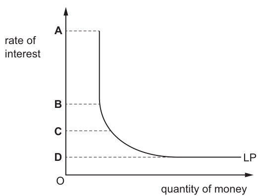
Options
A rate of interest A on Fig. 17.1
B rate of interest B on Fig. 17.1
C rate of interest C on Fig. 17.1
D rate of interest D on Fig. 17.1
Working
The liquidity trap occurs when the demand for money is perfectly interest inelastic, meaning the liquidity preference (LP) curve becomes perfectly horizontal. At this very low rate of interest, individuals prefer to hold money rather than bonds, as they expect interest rates to rise (and bond prices to fall) in the future. On the given diagram, the LP curve is horizontal at rate of interest D.
Answer
D
D
Background Concept
Liquidity preference theory, developed by John Maynard Keynes, explains the demand for money in an economy. The theory identifies three motives for holding money: the transactions motive (to fund everyday spending), the precautionary motive (to cover unexpected expenses), and the speculative motive (to take advantage of future changes in bond prices). The total demand for money (liquidity preference, LP) is inversely related to the rate of interest for the speculative motive: as interest rates rise, the opportunity cost of holding money (in the form of lost interest from bonds) increases, so people hold less money, and vice versa.
A liquidity trap is a specific situation in Keynesian theory that occurs when interest rates are very low. At this point, the speculative demand for money becomes perfectly elastic: people expect interest rates to rise in the future (which would cause bond prices to fall), so they choose to hold all their wealth as cash rather than buying bonds, no matter how much the central bank increases the money supply. This makes the LP curve perfectly horizontal at the low interest rate, meaning changes in the money supply have no effect on the interest rate, and monetary policy becomes ineffective at stimulating the economy.
Understanding the Question
This 1-mark multiple choice question asks you to identify which of the four labelled interest rates (A, B, C, D) on the liquidity preference diagram corresponds to the liquidity trap. The diagram shows the LP curve is downward-sloping at higher interest rates, then becomes perfectly horizontal at the lowest labelled rate, D. The question tests your recall of the definition of a liquidity trap and your ability to link that definition to the shape of the LP curve.
Approach
To answer this question, you need to:
- Recall the definition of a liquidity trap: the point where the LP curve is perfectly horizontal, due to perfectly interest-elastic speculative demand for money.
- Match this definition to the diagram: identify which interest rate corresponds to the horizontal section of the LP curve.
- Select the matching option.
Step-by-Step Reasoning
First, the liquidity trap is defined as the situation where the demand for money is perfectly elastic with respect to the interest rate, so the liquidity preference curve is horizontal. This occurs at very low interest rates, because at these rates, the expected capital gain from holding bonds (if interest rates fall further) is outweighed by the expected capital loss (if interest rates rise, which is seen as more likely when rates are already near zero). As a result, individuals will hold any additional money supplied by the central bank as cash, rather than using it to buy bonds, so the interest rate does not fall further even if the money supply increases.
Looking at the provided diagram:
- The vertical axis is the rate of interest, with A the highest rate and D the lowest.
- The LP curve is downward-sloping between rates B and C, as expected: higher interest rates reduce the quantity of money demanded.
- Below rate C, the LP curve becomes perfectly horizontal, extending to rate D. This horizontal section is the liquidity trap, because at these low interest rates, the quantity of money demanded is infinitely elastic: people will hold any amount of money at rate D, so the interest rate cannot fall below D no matter how much the money supply increases.
Therefore, the liquidity trap occurs at rate of interest D, so the correct option is D.
Key Takeaways
- The liquidity trap is a horizontal section of the liquidity preference (LP) curve, occurring at very low interest rates where speculative demand for money is perfectly elastic.
- In a liquidity trap, monetary policy (increasing the money supply) is ineffective at lowering interest rates further and stimulating investment and aggregate demand.
- The LP curve is downward-sloping at higher interest rates (where speculative demand is interest-elastic) and horizontal at the liquidity trap interest rate.
Common Mistakes
- Confusing the liquidity trap with the downward-sloping section of the LP curve: the liquidity trap is specifically the horizontal part, not the sloped part, so options A, B and C are incorrect.
- Misremembering the direction of the LP curve: the LP curve slopes downward (higher interest = lower money demand) except at the liquidity trap, where it is horizontal.
- Thinking the liquidity trap occurs at high interest rates: it only occurs at very low interest rates, when the opportunity cost of holding money is minimal and people expect rates to rise.
Things to Be Careful About
- Always link the definition of the liquidity trap to the shape of the LP curve: the key feature is the horizontal (perfectly elastic) segment, not just a low interest rate.
- Note that the liquidity trap is the lowest interest rate on the diagram, as it occurs when rates are near zero and cannot fall further.
- For 1-mark multiple choice questions, you only need to state the correct reasoning and select the right option; no extra detail is needed.
What is a likely consequence of an increase in government spending on education?
Options
A increase in the supply of unskilled labour
B increase in occupational mobility
C increase in the rate of unemployment
D increase in trade union power
Answer
Increased government spending on education improves the skills and qualifications of the workforce. This makes workers more adaptable to different types of jobs, thereby increasing occupational mobility.
Answer
B
B
Background Concept
Occupational mobility refers to the ease with which workers can move between different occupations or jobs. It is influenced by factors such as the level and type of skills, qualifications, training, and experience a worker possesses. Greater occupational mobility means workers can more readily switch to jobs where their labour is in higher demand, reducing structural unemployment and improving labour market efficiency.
Understanding the Question
The question asks for a likely consequence of an increase in government spending on education. The options are four possible outcomes: an increase in the supply of unskilled labour, an increase in occupational mobility, an increase in the rate of unemployment, or an increase in trade union power. The correct answer is the one that directly and logically follows from better education.
Approach
Consider the direct effect of more education spending: it raises the skill level of the workforce. More skilled workers are more adaptable and can perform a wider range of jobs. This directly increases occupational mobility. The other options are either opposite effects or unrelated.
Step-by-Step Reasoning
- Option A (increase in the supply of unskilled labour): Education spending typically reduces the number of unskilled workers by turning them into skilled workers. So this is the opposite of the likely consequence.
- Option B (increase in occupational mobility): Correct. With better education, workers gain transferable skills and qualifications that allow them to move between occupations more easily. For example, a worker with a general degree can apply for many different types of jobs, whereas an unskilled worker may be limited to a narrow range of manual roles.
- Option C (increase in the rate of unemployment): Education spending should reduce unemployment, especially structural unemployment, by equipping workers with the skills employers need. It does not cause unemployment.
- Option D (increase in trade union power): Trade union power depends on factors like membership density, legal framework, and the strategic position of workers in key industries. Education spending does not directly affect these.
Key Takeaways
- Government spending on education is a supply-side policy that improves human capital.
- One of its key microeconomic benefits is increasing the occupational mobility of labour, which helps reduce structural unemployment and improve labour market flexibility.
- Be careful not to confuse occupational mobility with geographical mobility (moving between locations) or with the overall supply of labour.
Common Mistakes
- Choosing A because of a mistaken belief that more education means more people in the labour force. In fact, education reduces the supply of unskilled labour, not increases it.
- Confusing occupational mobility with geographical mobility. The question specifically asks about the consequence of education, which primarily affects occupational mobility.
Things to Be Careful About
- Read each option carefully and think about the direct causal link. Education -> skills -> ability to change jobs -> occupational mobility.
- Do not overcomplicate the question. It is a straightforward application of basic labour market theory.
A country’s trade balance has worsened. The country has a fixed exchange rate.
Which additional changes for unemployment and price level are likely to follow?
Options
| the level of unemployment | the price level | |
|---|---|---|
| A | decreases | decreases |
| B | decreases | increases |
| C | increases | decreases |
| D | increases | increases |
Reasoning
A worsening trade balance means net exports (X – M) have fallen. This reduces aggregate demand (AD). Under a fixed exchange rate, the central bank must intervene to maintain the peg, so the exchange rate does not adjust to correct the imbalance.
With lower AD, the AD curve shifts left. In the AD/AS model, this reduces the equilibrium price level and reduces real output. Lower real output means firms need fewer workers, so unemployment rises.
Therefore unemployment increases and the price level decreases.
Answer
C
C
Background Concept
This question tests the link between the balance of payments and the domestic macroeconomy under a fixed exchange rate system. The key chain is:
-
Trade balance and AD: Net exports (X – M) are a component of aggregate demand (AD = C + I + G + (X – M)). A worsening trade balance — exports falling relative to imports — directly reduces AD.
-
Fixed exchange rate constraint: Under a fixed exchange rate, the central bank commits to keeping the currency's value at a target level. If the trade balance worsens, there is downward pressure on the currency (excess supply of the currency on forex markets). To maintain the peg, the central bank must buy its own currency using foreign reserves, which drains money from the economy and reinforces the contractionary effect. The exchange rate itself does not change, so there is no automatic correction via a cheaper currency boosting exports.
-
AD/AS model: A fall in AD shifts the AD curve leftwards. In the short run, this reduces both the price level (disinflation or deflation) and real output (a recessionary gap). Lower output means firms reduce employment, so unemployment rises.
Understanding the Question
The question presents a scenario: a country's trade balance has worsened, and it has a fixed exchange rate. It asks which combination of changes to unemployment and the price level is likely to follow. The four options pair increases and decreases for each variable. The key is to recognise that a worsening trade balance is a negative demand shock, and under a fixed exchange rate there is no offsetting depreciation to cushion the blow.
Approach
- Identify the direct effect of a worsening trade balance on AD.
- Recognise that under a fixed exchange rate, the exchange rate cannot adjust to offset the shock.
- Apply the AD/AS model: a leftward shift of AD reduces output (raising unemployment) and reduces the price level.
- Match this to the option that says unemployment increases and the price level decreases.
Step-by-Step Reasoning
- Step 1: A worsening trade balance means (X – M) falls. This is a reduction in one component of AD.
- Step 2: The fall in AD shifts the AD curve leftwards. In the AD/AS diagram, the new equilibrium is at a lower real GDP (Y) and a lower price level (P).
- Step 3: Lower real GDP means firms produce less, so they need fewer workers. This increases cyclical unemployment.
- Step 4: The lower price level reflects reduced demand-pull inflation (or outright deflation).
- Step 5: Under a fixed exchange rate, the central bank's intervention to defend the peg (selling foreign reserves, buying domestic currency) further tightens monetary conditions, reinforcing the contraction. There is no automatic depreciation to boost net exports.
Thus the outcome is: unemployment increases, price level decreases. This corresponds to option C.
Key Takeaways
- A worsening trade balance is a negative demand-side shock.
- Under a fixed exchange rate, the shock is not automatically offset by a change in the exchange rate.
- The AD/AS model is the essential tool for tracing the effects of changes in AD on output, employment, and the price level.
- Always consider the exchange rate regime when analysing the macroeconomic consequences of balance of payments changes.
Common Mistakes
- Assuming the exchange rate adjusts: Under a fixed exchange rate, the rate is pegged. Students sometimes incorrectly apply the logic of a floating rate (depreciation boosts exports, correcting the trade balance).
- Confusing the trade balance with the current account: The trade balance is a subset of the current account, but the question specifically says "trade balance", so focus on goods and services.
- Thinking unemployment falls: A fall in AD reduces output, so unemployment rises. Some students might think lower prices stimulate demand, but the initial shock is a reduction in AD, not an increase.
- Ignoring the fixed exchange rate: The question explicitly states the exchange rate is fixed. This is a crucial piece of information that changes the answer.
Things to Be Careful About
- Read the exchange rate regime carefully — it determines whether the exchange rate can adjust.
- Distinguish between a worsening trade balance (a fall in net exports) and an improvement (a rise in net exports).
- Remember that a fall in AD reduces both output and the price level in the short run (assuming an upward-sloping SRAS curve).
- The central bank's defence of a fixed peg is contractionary, reinforcing the initial demand shock.
What may prevent a government achieving a faster rate of growth of real GDP?
Options
A The multiplier has a small value.
B The consumer price index is below its target set by the central bank.
C The economy is operating on the vertical section of the long-run aggregate supply curve.
D There is a large negative output gap in the economy.
Answer
An economy operating on the vertical section of the long-run aggregate supply (LRAS) curve is at its full-employment level of output. In this situation, any increase in aggregate demand will only raise the price level, not real GDP, because the economy cannot produce more goods and services in the long run. Therefore, option C is correct.
Option A is incorrect because a small multiplier reduces the impact of any given increase in autonomous spending, but it does not prevent growth entirely — it just makes it smaller. Option B is incorrect because a CPI below target would typically encourage expansionary policy, not prevent growth. Option D is incorrect because a large negative output gap means the economy is below full capacity, so there is scope for demand-side policies to raise real GDP.
C
Background Concept
This question tests the distinction between demand-side and supply-side constraints on economic growth. Real GDP growth can be constrained either by insufficient aggregate demand (AD) or by the economy's productive capacity (aggregate supply). The long-run aggregate supply (LRAS) curve represents the economy's potential output when all resources are fully employed. In the classical/monetarist view, the LRAS is vertical at the full-employment level of output (Y*). Any increase in AD when the economy is at Y* will only cause inflation, not an increase in real GDP. The multiplier (option A) measures the size of the demand-side effect, but it is a constraint on the magnitude of growth, not a barrier to it. The output gap (option D) measures the difference between actual and potential output; a negative gap indicates spare capacity, which actually allows for demand-led growth.
Understanding the Question
The question asks: "What may prevent a government achieving a faster rate of growth of real GDP?" The key word is "prevent" — it implies a barrier that makes growth impossible, not just harder or smaller. The four options present different economic conditions. The correct answer is the one that describes a situation where, even if the government tries to stimulate the economy, real GDP cannot increase.
Approach
Evaluate each option against the criterion: does this condition make it impossible for real GDP to rise?
- Option A (small multiplier): A small multiplier means a given injection of spending has a smaller final effect on national income. But it does not prevent growth — it just reduces the size of the increase. The government could still achieve growth by using a larger stimulus. So this is not a "prevent" condition.
- Option B (CPI below target): A CPI below the central bank's target is a sign of low inflation or deflation. This typically gives the government or central bank room to use expansionary monetary or fiscal policy without fear of overshooting the inflation target. It does not prevent growth; it encourages it.
- Option C (vertical LRAS): If the economy is on the vertical section of the LRAS, it is at full employment. Any attempt to increase AD will only raise the price level (inflation) because the economy cannot produce more real output. This prevents an increase in real GDP in the long run. This is the correct answer.
- Option D (large negative output gap): A negative output gap means actual GDP is below potential GDP — there is spare capacity (unemployed resources). This is precisely the condition under which demand-side policies can raise real GDP without causing inflation. It does not prevent growth; it enables it.
Step-by-Step Reasoning
-
Identify the constraint on growth: Real GDP growth can be constrained by either demand or supply. The question asks for a preventative factor, so we need a supply-side constraint that makes it impossible to increase output.
-
Analyse Option C: The vertical LRAS curve represents the economy's maximum sustainable output. At this point, all factors of production are fully employed. Any increase in AD (e.g., through government spending or lower interest rates) will shift the AD curve rightwards along the vertical LRAS. The new equilibrium will have a higher price level but the same real GDP. Therefore, real GDP cannot increase. This is a genuine barrier.
-
Analyse Option A: The multiplier (k) = 1/(1-MPC) or 1/(MPW). A small multiplier (e.g., 1.2 instead of 2) means a given increase in autonomous spending (e.g., government spending G) leads to a smaller increase in equilibrium national income (Y = k * G). But the government can still increase Y by increasing G more. So a small multiplier does not prevent growth; it just makes it less efficient.
-
Analyse Option B: A CPI below target indicates that inflation is lower than desired. This is often a sign of weak demand. The government or central bank can use expansionary policies (lower interest rates, quantitative easing, increased government spending) to boost AD and raise real GDP without fear of causing excessive inflation. This condition does not prevent growth.
-
Analyse Option D: A large negative output gap means the economy is operating well below its potential. There is significant spare capacity (unemployed labour, idle factories). In this situation, an increase in AD can be met by increased production without causing inflation, because resources are available. This is the ideal condition for demand-led growth, not a barrier.
-
Conclusion: Only option C describes a situation where real GDP growth is impossible in the long run. The other options describe conditions that either reduce the effectiveness of policy (A) or are actually favourable for growth (B and D).
Key Takeaways
- The vertical LRAS curve represents the economy's full-employment output. At this point, demand-side policies cannot increase real GDP in the long run; they only cause inflation.
- A small multiplier reduces the impact of fiscal or monetary policy but does not prevent growth entirely.
- A negative output gap indicates spare capacity, which allows for demand-led growth.
- The distinction between demand-side and supply-side constraints is crucial for understanding the limits of macroeconomic policy.
Common Mistakes
- Confusing "small multiplier" with "zero multiplier": A small multiplier still allows for some growth; it just requires a larger stimulus. Students may incorrectly think a small multiplier prevents growth.
- Misinterpreting the vertical LRAS: Some students may think the vertical LRAS is a short-run concept or that it only applies to very high levels of output. In the classical model, it is the long-run constraint.
- Thinking a negative output gap prevents growth: A negative gap means the economy is below potential, so there is room to grow. This is a common misconception.
- Not reading the question carefully: The word "prevent" is strong. Students may choose an option that merely makes growth harder (like a small multiplier) rather than one that makes it impossible.
Things to Be Careful About
- The question asks what may prevent growth, not what makes it harder. The correct answer must describe a condition where growth is impossible, not just less effective.
- The vertical LRAS is a long-run concept. In the short run, the SRAS is upward-sloping, so an increase in AD can raise both output and the price level. But the question asks about a "faster rate of growth of real GDP" in general, and the vertical LRAS is the key long-run constraint.
- The multiplier (option A) is a demand-side concept. It affects the size of the demand-side effect, but it does not create a supply-side barrier.
- The output gap (option D) is a measure of spare capacity. A large negative gap means the economy is below full employment, so there is scope for growth without inflation.
A fall in domestic investment leads to an increase in unemployment.
Which other economic problem is likely to occur as a result?
Options
A an increase in interest rates on loans for house purchases
B an increase in the current account balance of payments deficit
C an increase in the government budget deficit
D an increase in the rate of price inflation
Answer
A fall in domestic investment reduces aggregate demand (AD). As AD falls, national income and output fall, leading to higher unemployment. Lower national income reduces tax revenues (income tax, corporation tax, VAT) and increases government spending on unemployment benefits and other welfare payments. The combination of lower tax receipts and higher transfer payments automatically increases the government budget deficit (or reduces a surplus).
Answer
C
C
Background Concept
Investment (I) is a component of aggregate demand (AD = C + I + G + X - M). A fall in investment directly reduces AD. Through the multiplier process, the initial fall in AD leads to a larger final fall in national income (Y). As Y falls, unemployment rises because firms need fewer workers to produce the lower level of output. The government's budget position is affected by automatic stabilisers: tax revenues are a positive function of income (they fall when income falls), and transfer payments (e.g. unemployment benefits) are a negative function of income (they rise when income falls). The budget deficit = G - T; if T falls and G (including transfers) rises, the deficit increases.
Understanding the Question
The question states: "A fall in domestic investment leads to an increase in unemployment." It then asks which OTHER economic problem is likely to occur as a result. The key word is "other" — we already know unemployment rises. We must identify which of the four options is a likely consequence of the same initial fall in investment. The question tests the ability to trace the macroeconomic effects of a demand-side shock through the circular flow and to distinguish between likely and unlikely outcomes.
Approach
- Identify the initial change: a fall in domestic investment (a fall in I).
- Trace the effect on AD and national income (Y).
- Consider the effect on each of the four options:
- A: interest rates on loans for house purchases (mortgage rates).
- B: the current account balance of payments deficit.
- C: the government budget deficit.
- D: the rate of price inflation.
- Use economic reasoning to determine which is the most likely consequence.
Step-by-Step Reasoning
Step 1: The initial shock
A fall in domestic investment means firms spend less on capital goods (machinery, factories, etc.). This directly reduces the I component of AD.
Step 2: Effect on AD and national income
AD falls. With a downward multiplier, the fall in national income (Y) is larger than the initial fall in I. Lower Y means lower output, so firms need fewer workers — hence unemployment rises (as stated in the question).
Step 3: Evaluate each option
Option A: an increase in interest rates on loans for house purchases
Interest rates are determined by monetary policy (set by the central bank) or by market forces of demand and supply of loanable funds. A fall in investment and rising unemployment would typically lead the central bank to LOWER interest rates to stimulate the economy, not raise them. So this is unlikely. (Even if the central bank kept rates unchanged, mortgage rates would not rise as a direct consequence of lower investment.)
Option B: an increase in the current account balance of payments deficit
The current account balance = exports (X) - imports (M). A fall in national income reduces spending on imports (since M is a positive function of Y). So imports fall, which IMPROVES the current account balance (reduces a deficit or increases a surplus). Therefore, the deficit is likely to DECREASE, not increase. This option is incorrect.
Option C: an increase in the government budget deficit
As Y falls:
- Tax revenues (T) fall: income tax, corporation tax, VAT all decline because incomes, profits, and spending are lower.
- Government spending on transfer payments (part of G) rises: more people claim unemployment benefits and other welfare payments.
The budget deficit = G - T. With T falling and G (including transfers) rising, the deficit INCREASES. This is a direct and automatic consequence — the automatic stabilisers. This is the correct answer.
Option D: an increase in the rate of price inflation
A fall in AD reduces demand-pull inflationary pressure. With lower demand, firms are less able to raise prices; indeed, they may cut prices to attract customers. Inflation is likely to FALL, not rise. This option is incorrect.
Conclusion: Only option C is a likely consequence of a fall in investment that raises unemployment.
Key Takeaways
- Investment is a component of AD; a fall in investment reduces AD and national income.
- Automatic stabilisers mean that a fall in income automatically worsens the government budget deficit (lower tax revenue + higher transfer spending).
- A fall in income reduces imports, improving the current account.
- A fall in AD reduces inflationary pressure.
- Monetary policy typically responds to a downturn by lowering interest rates, not raising them.
Common Mistakes
- Confusing the effect on the current account: some students think lower income means less exports, but exports are determined by foreign income, not domestic income. The relevant effect is on imports.
- Thinking that a fall in investment causes inflation because investment is "spending" — but it's a fall in spending, so it reduces demand-pull inflation.
- Assuming interest rates always rise when the economy weakens — in reality, central banks cut rates to stimulate the economy.
Things to Be Careful About
- Read the question carefully: it asks for the "other" problem, so the answer must be a consequence of the same initial fall in investment.
- Distinguish between automatic changes (like the budget deficit) and policy responses (like interest rate changes). The question asks what is "likely to occur as a result" — automatic effects are more certain than policy responses.
- Remember that imports are a function of income: M = mY, so when Y falls, M falls.
To overcome deflation in an economy the government increases the size of its budget deficit and funds this by increasing the money supply.
What is most likely to reduce the effectiveness of these measures?
Options
A a high marginal propensity to save
B a rise in business confidence
C an inelastic demand for money
D low cash deposit ratios for commercial banks
Answer
The government is using expansionary fiscal policy (increasing the budget deficit) and expansionary monetary policy (increasing the money supply).
A high marginal propensity to save (MPS) reduces the size of the multiplier. A smaller multiplier means that any given increase in government spending (from the larger deficit) will generate a smaller final increase in national income. This directly reduces the effectiveness of the fiscal stimulus.
A high MPS also means that the extra money created by the monetary expansion is more likely to be saved rather than spent on goods and services. In the quantity theory of money (MV = PT), if the extra money (M) is held as idle balances (so V falls), the increase in nominal spending (PT) is muted. Therefore, the monetary stimulus is also weakened.
Option A is the only factor that reduces the effectiveness of both policies.
Answer
A
A
Background Concept
This question tests two core macroeconomic mechanisms and how they interact.
1. The Multiplier and the Marginal Propensity to Save (MPS)
The multiplier (k) measures the final change in national income resulting from an initial change in aggregate demand (e.g., government spending). The formula for a simple closed economy with no government is:
k = 1 / MPS
A higher MPS means a larger proportion of any additional income is saved rather than spent. This reduces the size of the multiplier. For example, if MPS = 0.2, k = 5. If MPS = 0.5, k = 2. A given increase in government spending will therefore have a smaller final impact on national income when the MPS is high.
2. The Quantity Theory of Money (MV = PT)
This identity states that the money supply (M) multiplied by the velocity of circulation (V) equals the price level (P) multiplied by the volume of transactions (T). In its simplest form, it suggests that an increase in the money supply (M) will lead to a proportional increase in nominal spending (PT), assuming V and T are constant. However, if the public chooses to hold the extra money as idle balances (saving it rather than spending it), the velocity of circulation (V) falls. The increase in nominal spending is then smaller than the increase in the money supply.
Understanding the Question
The question describes a government trying to overcome deflation (falling prices) using two policies simultaneously:
- Fiscal policy: Increasing the budget deficit (e.g., by increasing government spending or cutting taxes).
- Monetary policy: Funding this deficit by increasing the money supply (effectively printing money or using quantitative easing).
The question asks which factor is most likely to reduce the effectiveness of these measures. We need to find the option that weakens the impact of both the fiscal and monetary stimulus.
Approach
We must evaluate each option in turn, considering its effect on both the fiscal and monetary transmission mechanisms.
- Option A: A high marginal propensity to save (MPS). This directly reduces the multiplier, weakening the fiscal stimulus. It also means the extra money from the monetary expansion is more likely to be saved, reducing its impact on spending.
- Option B: A rise in business confidence. This would likely increase the effectiveness of the policies, as businesses would be more willing to invest in response to the stimulus.
- Option C: An inelastic demand for money. This means that a small change in the interest rate is needed to make people hold a larger money supply. This would make monetary policy more effective, not less.
- Option D: Low cash deposit ratios for commercial banks. This means banks have more capacity to lend, which would increase the effectiveness of the monetary stimulus through the credit creation multiplier.
Option A is the only one that weakens both policies.
Step-by-Step Reasoning
-
Identify the two policies: The government is using expansionary fiscal policy (larger deficit) and expansionary monetary policy (increasing money supply).
-
Analyze Option A (High MPS):
- Effect on Fiscal Policy: The multiplier (k = 1/MPS) is smaller. A given increase in government spending (G) leads to a smaller final increase in national income (Y). The fiscal stimulus is less effective.
- Effect on Monetary Policy: When the central bank increases the money supply, it hopes this will lead to more spending. However, if people have a high MPS, they will save a large portion of any new money they receive. This reduces the velocity of circulation (V). In the equation MV = PT, if M increases but V falls, the increase in nominal spending (PT) is muted. The monetary stimulus is less effective.
- Conclusion for A: This option reduces the effectiveness of both policies.
-
Analyze Option B (Rise in business confidence):
- Effect on Fiscal Policy: Higher confidence makes businesses more likely to invest. This could amplify the multiplier effect of the fiscal stimulus, making it more effective.
- Effect on Monetary Policy: Higher confidence makes businesses more likely to borrow and invest the new money, increasing its velocity. This makes the monetary stimulus more effective.
- Conclusion for B: This option increases effectiveness, not reduces it.
-
Analyze Option C (Inelastic demand for money):
- The demand for money is the desire to hold cash balances. If it is inelastic, it means people's demand for money is not very sensitive to changes in the interest rate.
- Effect on Monetary Policy: To increase the money supply, the central bank buys bonds, which pushes bond prices up and interest rates down. If the demand for money is inelastic, a very small fall in the interest rate is enough to make people willing to hold the new money. This means the policy is very effective at lowering interest rates and stimulating spending. It does not reduce effectiveness.
- Effect on Fiscal Policy: This has no direct bearing on the fiscal multiplier.
- Conclusion for C: This option does not reduce the effectiveness of the policies.
-
Analyze Option D (Low cash deposit ratios for commercial banks):
- The cash deposit ratio is the fraction of deposits a bank must hold as reserves. A low ratio means banks have more freedom to lend.
- Effect on Monetary Policy: When the central bank increases the monetary base (e.g., by buying bonds), banks can use this new money to create more credit through the credit creation multiplier. A low cash deposit ratio means a higher credit multiplier, making the monetary stimulus more effective.
- Effect on Fiscal Policy: This has no direct bearing on the fiscal multiplier.
- Conclusion for D: This option increases the effectiveness of monetary policy.
-
Final Judgement: Only Option A (a high marginal propensity to save) reduces the effectiveness of both the expansionary fiscal and monetary policies.
Key Takeaways
- A high MPS reduces the multiplier, weakening fiscal policy.
- A high MPS also reduces the velocity of circulation, weakening monetary policy.
- The effectiveness of a policy depends on the economic context and the values of key parameters like the MPS.
- Always consider how a given factor affects the specific transmission mechanism of each policy.
Common Mistakes
- Confusing MPS with MPC: A high MPS is the same as a low MPC. A low MPC also reduces the multiplier.
- Thinking a high MPS only affects fiscal policy: Many students forget that the velocity of money is also affected by the propensity to save.
- Misunderstanding the demand for money: An inelastic demand for money makes monetary policy more powerful, not less.
- Confusing cash deposit ratios with reserve requirements: A low ratio means banks can lend more, which is expansionary.
Things to Be Careful About
- Read the question carefully: it asks for what is most likely to reduce effectiveness.
- Consider the impact on both policies, not just one.
- Remember the formula for the multiplier (k = 1/MPS) and the quantity theory of money (MV = PT).
- Distinguish between factors that affect the size of the stimulus (multiplier) and factors that affect the transmission of the stimulus (velocity, credit creation).
The diagram shows the aggregate demand, AD, and aggregate supply, AS, curves for an economy. The initial equilibrium is at point E. There is a revaluation of the exchange rate.
If the Marshall-Lerner rule applies, which point on the diagram would show the new long-run equilibrium?
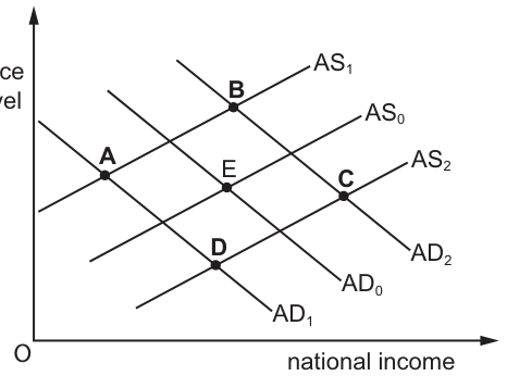
Options
A point A on Fig. 23.1
B point B on Fig. 23.1
C point C on Fig. 23.1
D point D on Fig. 23.1
A revaluation of the exchange rate means the domestic currency appreciates in value. This makes exports more expensive for foreign buyers and imports cheaper for domestic consumers. Consequently, the volume of exports falls and the volume of imports rises, causing net exports (X - M) to decrease. Because net exports are a component of aggregate demand (AD = C + I + G + X - M), aggregate demand falls and shifts leftwards from AD0 to AD1.
The Marshall-Lerner rule states that a change in the exchange rate will affect the trade balance in the expected direction only if the sum of the price elasticities of demand for exports and imports is greater than 1. If this condition applies to a revaluation, the quantity effects dominate the price effects, confirming that the trade balance worsens and net exports fall. This reinforces the leftward shift in AD.
In the long run, the economy returns to its potential output level, represented by the aggregate supply curve AS0. The new long-run equilibrium occurs where the new aggregate demand curve (AD1) intersects the original aggregate supply curve (AS0). This is point D.
Answer
D
D
Background Concept
An exchange rate revaluation is a deliberate upward adjustment of a currency's value within a fixed or managed exchange rate system, making the domestic currency stronger relative to foreign currencies. This affects the relative prices of exports and imports: exports become more expensive for foreigners and imports become cheaper for domestic residents. The Marshall-Lerner condition examines whether the sum of the price elasticities of demand for exports and imports exceeds 1. If it does, a change in the exchange rate improves the trade balance following a depreciation, or worsens it following a revaluation (appreciation), because the percentage change in quantities demanded exceeds the percentage change in prices.
In the AD/AS model, aggregate demand comprises consumption (C), investment (I), government spending (G), and net exports (X - M). A fall in net exports reduces AD, shifting the AD curve leftward. The long-run aggregate supply curve (here represented by AS0) indicates the economy's potential output at full employment. A long-run equilibrium occurs where AD intersects this long-run supply curve.
Understanding the Question
The question presents an AD/AS diagram with initial equilibrium at point E (intersection of AD0 and AS0). It states that there is a revaluation of the exchange rate and that the Marshall-Lerner rule applies. The task is to identify which point (A, B, C, or D) represents the new long-run equilibrium.
The key elements are: (1) the direction of the AD shift caused by a revaluation, (2) the role of the Marshall-Lerner condition in confirming this direction, and (3) the location of the long-run equilibrium after this demand-side shock. The command word is implicit in the multiple-choice format, requiring application of theory to the diagram.
Approach
- Determine the effect of a revaluation on net exports and AD.
- Confirm the direction of the AD shift using the Marshall-Lerner condition.
- Identify the long-run aggregate supply curve (AS0) and locate the intersection with the new AD curve.
- Match this intersection to one of the labelled points.
The Marshall-Lerner condition is crucial here because it rules out the J-curve effect or any perverse short-run outcome; it guarantees that the trade balance moves in the direction predicted by the price change. For a revaluation, this means net exports fall.
Step-by-Step Reasoning
First, a revaluation means the domestic currency appreciates. UK goods become more expensive for overseas buyers, so export volumes decline. Foreign goods become cheaper for UK residents, so import volumes rise. The value of exports falls and the value of imports rises, so net exports (X - M) decrease.
Second, because net exports are a component of AD, a decrease in net exports causes AD to fall. The AD curve shifts leftward from AD0 to AD1. The Marshall-Lerner condition confirms this outcome: if the sum of the elasticities of demand for exports and imports is greater than 1, the percentage fall in export revenue and rise in import expenditure is proportionally larger than the price change, ensuring the trade balance worsens and AD definitely shifts left.
Third, in the long run, the economy returns to its potential output level. The curve AS0 represents the long-run aggregate supply (or the supply capacity to which the economy returns). The new long-run equilibrium is therefore at the intersection of the new AD curve (AD1) and the original AS curve (AS0).
Looking at the diagram, the intersection of AD1 and AS0 is point D. Point A would require AS to shift left as well, which does not result from a revaluation. Point B is on the original AD curve. Point C is on AD2, which is to the right of AD0, implying an increase in AD (consistent with depreciation, not revaluation). Thus, point D is the correct new long-run equilibrium.
Key Takeaways
- A revaluation (appreciation) reduces net exports and shifts AD leftward.
- The Marshall-Lerner condition determines the direction of change in the trade balance following an exchange rate change; for a revaluation, if it applies, the trade balance worsens.
- Long-run equilibrium in the AD/AS model occurs where the AD curve intersects the long-run aggregate supply curve (AS0 in this diagram).
- After a leftward shift in AD, the new long-run equilibrium is at a lower price level but the same real output (if AS0 is vertical) or lower output and lower price level (if AS0 is upward sloping), specifically at point D.
Common Mistakes
- Confusing revaluation with depreciation: depreciation would shift AD rightward to AD2, leading to point C, which is incorrect.
- Misapplying the Marshall-Lerner rule: some students think the rule always shifts AD right, but it depends on whether the currency is depreciating or revaluing.
- Selecting point A: this incorrectly assumes that a revaluation also shifts the aggregate supply curve leftward. Revaluation is a demand-side shock; it does not directly shift AS in the long run.
- Ignoring the "long-run" qualifier: point D is on the original AS curve, reflecting the economy's return to potential output.
Things to Be Careful About
- Revaluation is an appreciation (exchange rate rises), not a depreciation.
- The Marshall-Lerner condition applies to the trade balance effect: for a revaluation, it confirms that net exports fall.
- In the long run, the aggregate supply curve does not shift in response to a demand-side shock like a revaluation; the economy returns to its original supply capacity (AS0).
- Ensure you identify the correct intersection: AD1 (the leftward-shifted curve) with AS0 (the original supply curve) gives point D.
What does the Kuznets curve show about the relationship between economic development and inequality?
Options
A the Gini coefficient initially falls as countries develop from low to high income levels
B the Gini coefficient initially rises as countries develop from low to high income levels
C there is always a negative relationship between GDP per capita and the Gini coefficient
D there is always a positive relationship between GDP per capita and the Gini coefficient
Answer
The Kuznets curve shows that as an economy develops from low to high income levels, inequality (measured by the Gini coefficient) initially rises, peaks, and then falls. Therefore, the correct option is B.
B
Background Concept
The Kuznets curve, proposed by economist Simon Kuznets in the 1950s, is a hypothesis about the relationship between economic development (measured by GDP per capita) and income inequality (often measured by the Gini coefficient). Kuznets argued that in the early stages of industrialisation, inequality increases as a small portion of the population benefits from new opportunities in the industrial sector while the majority remains in low-productivity agriculture. As development continues and the industrial sector expands to absorb more workers, inequality eventually decreases, creating an inverted-U shape when plotted on a graph.
Understanding the Question
This multiple-choice question asks what the Kuznets curve shows about the relationship between economic development and inequality. The key is to recall the specific shape and direction of the relationship: it is not a simple positive or negative correlation throughout, but rather a pattern where inequality first rises and then falls. The Gini coefficient is a common measure of inequality, where 0 represents perfect equality and 1 (or 100) represents perfect inequality.
Approach
To answer this question, you need to recall the defining characteristic of the Kuznets curve: its inverted-U shape. This means that as GDP per capita rises from low to high levels, the Gini coefficient initially increases, reaches a peak, and then decreases. Options C and D suggest a constant relationship (always negative or always positive), which contradicts the inverted-U shape. Option A describes the opposite pattern (inequality initially falls), which is incorrect. Option B correctly states that the Gini coefficient initially rises.
Step-by-Step Reasoning
- Recall the Kuznets curve hypothesis: The Kuznets curve is an inverted-U shaped curve. On the x-axis is economic development (usually GDP per capita), and on the y-axis is income inequality (usually the Gini coefficient).
- Analyse the shape: As development begins from a low base, inequality rises. This is because the benefits of early industrialisation are concentrated among a few (e.g., factory owners, skilled workers in new industries). The majority of the population remains in traditional agriculture with lower incomes, widening the gap.
- Identify the turning point: After a certain level of development, inequality starts to fall. This is attributed to factors such as the spread of education, the expansion of the industrial sector to include more workers, the development of social safety nets, and political pressure for redistribution.
- Evaluate the options:
- Option A: States the Gini coefficient initially falls. This is the opposite of the Kuznets curve's first phase. Incorrect.
- Option B: States the Gini coefficient initially rises. This matches the first phase of the Kuznets curve. Correct.
- Option C: States there is always a negative relationship. This implies inequality falls continuously, which is not what the Kuznets curve shows. Incorrect.
- Option D: States there is always a positive relationship. This implies inequality rises continuously, which is not what the Kuznets curve shows. Incorrect.
Key Takeaways
- The Kuznets curve is an inverted-U relationship between economic development and income inequality.
- Inequality initially rises during early industrialisation and then falls as the economy matures.
- The Gini coefficient is a standard measure of income inequality.
- Be careful not to confuse the Kuznets curve with a simple linear relationship.
Common Mistakes
- Choosing a linear relationship: Students often mistakenly think the relationship is always positive or always negative, ignoring the inverted-U shape. This leads to selecting options C or D.
- Reversing the direction: Some students may remember the curve but think inequality initially falls, leading them to choose option A.
- Confusing the Kuznets curve with the Environmental Kuznets Curve (EKC): The EKC hypothesises a similar inverted-U relationship between economic development and environmental degradation. Ensure you are answering about the original Kuznets curve on income inequality.
Things to Be Careful About
- The question asks what the Kuznets curve shows, not what it proves. It is an empirical observation or hypothesis, not a law.
- Pay attention to the word "initially" in options A and B. This is the key differentiator for the first phase of the curve.
- The Gini coefficient is the standard measure, but the question could also refer to other inequality measures. The principle of the inverted-U shape remains the same.
Which statement about the components of the balance of payments is correct?
Options
A The current account consists of transactions in goods, services, investment income and remittances between countries.
B The current account consists of transactions in goods, services, and portfolio investment between countries.
C The financial account consists of transactions in financial assets, investment income and remittances between countries.
D The financial account consists of transactions in fixed assets, investment income and the balancing item between countries.
Answer
The current account records transactions in goods (visible trade), services (invisible trade), investment income (profits, dividends, interest from overseas assets), and current transfers (remittances, grants). The financial account records transactions in financial assets (shares, bonds, loans, FDI, reserves).
Option A correctly lists the components of the current account.
Answer
A
A
Background Concept
The balance of payments is a record of all economic transactions between residents of one country and the rest of the world over a period. It is divided into two main accounts:
- Current account: records flows of goods, services, income, and current transfers.
- Financial account (formerly capital account in some definitions): records flows of financial assets (portfolio investment, direct investment, reserves, other investment).
A third, smaller capital account (in the modern IMF definition) records capital transfers and acquisition/disposal of non-produced, non-financial assets, but this is not tested in the options here.
Understanding the Question
The question asks which statement correctly describes the components of the balance of payments. It tests precise knowledge of what belongs in the current account versus the financial account. The distractors mix up components between the two accounts.
Approach
Recall the standard classification:
- Current account: goods, services, primary income (investment income), secondary income (current transfers/remittances).
- Financial account: direct investment, portfolio investment, financial derivatives, reserve assets, other investment.
Then check each option against this classification.
Step-by-Step Reasoning
Option A: "The current account consists of transactions in goods, services, investment income and remittances between countries."
- Goods: visible trade (exports and imports of physical items). Correct.
- Services: invisible trade (tourism, transport, insurance, financial services). Correct.
- Investment income: profits, dividends, interest earned on overseas assets. Correct.
- Remittances: current transfers (money sent by migrant workers to their home country). Correct.
- This is the correct definition.
Option B: "The current account consists of transactions in goods, services, and portfolio investment between countries."
- Portfolio investment (purchase of shares and bonds) belongs in the financial account, not the current account. Incorrect.
Option C: "The financial account consists of transactions in financial assets, investment income and remittances between countries."
- Investment income and remittances belong in the current account, not the financial account. Incorrect.
Option D: "The financial account consists of transactions in fixed assets, investment income and the balancing item between countries."
- "Fixed assets" is ambiguous but typically refers to physical capital (machinery, buildings) which is recorded in the current account as goods trade. Investment income is current account. The balancing item (errors and omissions) is a separate entry, not part of the financial account. Incorrect.
Key Takeaways
- The current account records income flows (goods, services, investment income, transfers).
- The financial account records asset flows (financial investments, loans, reserves).
- Investment income is NOT a financial asset; it is a return on an asset and belongs in the current account.
- Remittances are current transfers, not financial transactions.
Common Mistakes
- Confusing investment income (current account) with portfolio investment (financial account).
- Thinking remittances are financial flows because they involve money moving between countries — they are current transfers because they are unilateral and not in exchange for an asset.
- Mixing up the old terminology where "capital account" was used for what is now the financial account.
Things to Be Careful About
- The IMF's Balance of Payments Manual (BPM6) standardises the classification: current account, capital account, financial account. The question uses the modern convention.
- "Portfolio investment" is a financial account item; "investment income" is a current account item. They sound similar but are distinct.
- The balancing item (errors and omissions) is a separate entry to make the accounts balance, not part of either main account.
Which statement describes a multinational company (MNC)?
Options
A A firm that avoids paying indirect taxes.
B A firm that conducts operations in different countries.
C A firm that experiences diseconomies of scale at low levels of output.
D A firm that trades internationally.
Answer
B
B
Background Concept
A multinational company (MNC) is a firm that owns or controls production facilities or other operations in more than one country. The key distinguishing feature is that it engages in foreign direct investment (FDI) — it does not merely export goods to other countries but actually establishes a physical presence (factories, offices, subsidiaries) abroad. This is different from a firm that only trades internationally by exporting or importing, which does not make it multinational.
Understanding the Question
The question asks which statement correctly describes a multinational company. Four options are given, and only one is accurate. The correct answer must capture the essential characteristic that sets MNCs apart from other firms that participate in international trade.
Approach
Read each option carefully and compare it against the standard definition of an MNC. Eliminate options that are either false or describe a different type of firm.
Step-by-Step Reasoning
-
Option A: "A firm that avoids paying indirect taxes." This is not a defining feature of an MNC. Many firms, both domestic and multinational, may engage in tax avoidance or tax planning, but this is not what makes a company multinational. Incorrect.
-
Option B: "A firm that conducts operations in different countries." This is the correct definition. An MNC has operations (production, assembly, sales, research, etc.) in multiple countries. This is the core characteristic.
-
Option C: "A firm that experiences diseconomies of scale at low levels of output." Diseconomies of scale occur when a firm becomes too large and average costs start to rise. This is a concept from the theory of the firm and is not specific to MNCs. Many small firms also experience diseconomies of scale at low output. Incorrect.
-
Option D: "A firm that trades internationally." This describes any firm that exports or imports goods. A firm can trade internationally without having any operations abroad — it may simply sell its products to foreign customers or buy inputs from foreign suppliers. Such a firm is an international trader but not a multinational. Incorrect.
Therefore, the only correct description is B.
Key Takeaways
- The defining feature of an MNC is that it has operations (production or other business activities) in multiple countries.
- International trade (exporting/importing) alone does not make a firm multinational.
- MNCs are a key feature of globalisation and are associated with foreign direct investment.
Common Mistakes
- Confusing "trading internationally" with "being multinational." Many students pick D because they think any firm that sells abroad is an MNC. However, an MNC must have a physical presence abroad.
- Thinking that tax avoidance is a defining characteristic of MNCs. While some MNCs do engage in tax planning, it is not part of the definition.
Things to Be Careful About
- Read the options precisely. Option D says "trades internationally" — this is a broader category that includes many firms that are not MNCs.
- Remember that the definition of an MNC focuses on the location of its operations, not just its market.
What occurs in a monetary union?
Options
A Countries have the same currency.
B Countries use the same fiscal policy.
C Countries have the same domestic rates of sales tax.
D The government budget in each country is balanced.
Answer
A monetary union is a form of economic integration in which member countries adopt a common currency and a single monetary policy, typically managed by a shared central bank. The key feature is a shared currency, not harmonised fiscal policy, tax rates, or balanced budgets.
Answer
A
A
Background Concept
Economic integration refers to the process by which countries reduce trade barriers and coordinate their economic policies. The main stages, in increasing order of integration, are:
- Free trade area: no internal tariffs, but each country sets its own external tariffs.
- Customs union: free trade area plus a common external tariff.
- Common market: customs union plus free movement of labour and capital.
- Monetary union: common market plus a single currency and a single monetary policy.
- Full economic union: monetary union plus harmonised fiscal and other economic policies.
A monetary union therefore involves giving up national control over monetary policy and exchange rates in favour of a shared currency and central bank. Fiscal policy (taxation and government spending) remains largely under national control, though there may be coordination rules.
Understanding the Question
This is a straightforward multiple-choice question testing the definition of a monetary union. The question asks: "What occurs in a monetary union?" and provides four options. The correct answer is the one that describes the essential, defining feature of a monetary union.
Approach
Recall the definition of a monetary union from the syllabus. Identify which of the four options matches that definition. The other options describe features that are not part of a monetary union (common fiscal policy, same sales tax rates, balanced budgets).
Step-by-Step Reasoning
-
Option A: "Countries have the same currency." This is the core of a monetary union. Members adopt a single currency (e.g., the euro in the Eurozone) and a single monetary policy set by a common central bank (e.g., the European Central Bank). This is correct.
-
Option B: "Countries use the same fiscal policy." Fiscal policy (taxation and government spending) is not necessarily harmonised in a monetary union. While there may be coordination rules (e.g., the Stability and Growth Pact in the EU), each country retains its own fiscal policy. This is not a defining feature.
-
Option C: "Countries have the same domestic rates of sales tax." Sales tax rates (like VAT) are not part of a monetary union. They can vary widely among members. This is incorrect.
-
Option D: "The government budget in each country is balanced." A balanced budget is not a requirement of a monetary union. Countries can run deficits or surpluses. This is incorrect.
Therefore, the correct answer is A.
Key Takeaways
- A monetary union is defined by a shared currency and a single monetary policy.
- It does not require harmonised fiscal policy, tax rates, or balanced budgets.
- Distinguish monetary union from other forms of economic integration (free trade area, customs union, common market, full economic union).
Common Mistakes
- Confusing a monetary union with a fiscal union or full economic union. Students may think that a monetary union requires common fiscal policy, which is not true.
- Thinking that a monetary union requires all members to have the same tax rates or balanced budgets.
Things to Be Careful About
- Read the options carefully. The question asks what "occurs" in a monetary union, meaning what is necessarily true. Only option A is necessarily true.
- Remember that the euro area is the classic example: countries share the euro and ECB monetary policy, but each sets its own taxes and budgets (within some agreed limits).
What is the main role of the World Bank?
Options
A to ensure that exchange rate systems are working efficiently
B to help countries enter international markets where trade barriers exist
C to offer short-term assistance to countries with balance of payments problems
D to provide low-interest loans to developing countries for infrastructure projects
Answer
The World Bank's main role is to provide low-interest loans to developing countries for infrastructure projects. This distinguishes it from the IMF, which offers short-term assistance for balance of payments problems.
Answer
D
D
Background Concept
The World Bank and the International Monetary Fund (IMF) are two key international financial institutions created at the Bretton Woods Conference in 1944. While they are often mentioned together, they have distinct mandates. The World Bank focuses on long-term economic development and poverty reduction by providing financial and technical assistance for specific projects (e.g., building roads, dams, schools, hospitals) in developing countries. The IMF, in contrast, focuses on the stability of the international monetary system and provides short-term loans to countries facing balance of payments crises, often with conditions attached.
Understanding the Question
This is a straightforward multiple-choice question asking for the main role of the World Bank. The four options present plausible but incorrect roles for the other institutions or for the World Bank itself. The correct answer is the one that accurately describes the World Bank's primary function.
Approach
Recall the core function of the World Bank: providing long-term, low-interest loans and grants for development projects in poorer countries. Then eliminate the options that describe the roles of other institutions (like the IMF) or that are not the World Bank's main focus.
Step-by-Step Reasoning
- Option A describes a function of the IMF, which monitors exchange rate systems and provides policy advice. The World Bank does not do this.
- Option B is not a direct role of either institution. While the World Bank may help countries improve their trade capacity, its main role is not specifically to help them enter markets where trade barriers exist.
- Option C describes the IMF's role of providing short-term assistance to countries with balance of payments problems. The World Bank provides long-term loans, not short-term balance of payments support.
- Option D correctly identifies the World Bank's main role: providing low-interest loans to developing countries for infrastructure projects (and other development projects). This is its core mandate.
Key Takeaways
- The World Bank = long-term development loans for projects (infrastructure, education, health).
- The IMF = short-term loans for balance of payments stability and exchange rate system oversight.
- Knowing the distinct roles of these two institutions is a common exam point.
Common Mistakes
- Confusing the World Bank with the IMF. Many students mix up their functions, especially because both are involved in lending to countries. The key difference is the time horizon and purpose: long-term development vs. short-term balance of payments.
- Thinking the World Bank's main role is to help with trade barriers or exchange rates, which are more the domain of the WTO and IMF respectively.
Things to Be Careful About
- Read each option carefully. The question asks for the "main" role, so even if the World Bank does some of the other things (e.g., indirectly helping with trade), the primary function is what matters.
- Remember that the World Bank group includes several institutions (IBRD, IDA, IFC, etc.), but the core function remains development lending to poorer countries.
There is a rise in the domestic rate of interest in an economy. This economy has a fixed exchange rate.
What would be the impact on the current and financial accounts of the balance of payments?
Options
| current account | financial account | |
|---|---|---|
| A | improves | improves |
| B | improves | worsens |
| C | worsens | improves |
| D | worsens | worsens |
Answer
A rise in the domestic rate of interest makes domestic financial assets more attractive to foreign investors. This increases capital inflows, improving the financial account.
Under a fixed exchange rate, the central bank must maintain the currency's value. The capital inflow puts upward pressure on the exchange rate, so the central bank sells domestic currency and buys foreign currency to keep the rate fixed. This intervention increases the domestic money supply, which is inflationary. To sterilise this, the central bank may sell bonds, raising interest rates further. The higher interest rate reduces aggregate demand (consumption and investment), which reduces import spending. Lower imports improve the current account.
Therefore, both the current account and the financial account improve.
Answer
A
A
Background Concept
The balance of payments records all transactions between residents of one economy and the rest of the world. It has two main accounts:
- Current account: records trade in goods and services, primary income (investment income, compensation of employees), and secondary income (transfers). A deficit means the country spends more on foreign goods, services, and income than it earns from abroad.
- Financial account: records cross-border financial assets and liabilities, including foreign direct investment (FDI), portfolio investment (shares, bonds), and other investment (bank loans, deposits). A surplus means more capital flows into the country than out.
Under a fixed exchange rate, the central bank commits to keeping the currency's value within a narrow band against another currency (or a basket). To do this, it must intervene in the foreign exchange market: buying its own currency when it weakens, selling it when it strengthens. This intervention directly affects the domestic money supply and, through the monetary transmission mechanism, affects aggregate demand and the current account.
Understanding the Question
The question presents a scenario: a rise in the domestic rate of interest in an economy that operates a fixed exchange rate. It asks for the impact on both the current account and the financial account of the balance of payments. The answer choices are combinations of 'improves' and 'worsens' for each account.
The key is to trace the chain of causation step by step, remembering that under a fixed exchange rate, the central bank's actions to maintain the peg link the financial account to the current account.
Approach
-
First step: financial account. A higher domestic interest rate makes domestic bonds and deposits more attractive to foreign investors. They buy more of them, increasing capital inflows. This directly improves the financial account (more money coming in than going out).
-
Second step: exchange rate pressure. The increased demand for domestic currency (to buy domestic assets) pushes its value up. Under a fixed exchange rate, the central bank must prevent this appreciation. It does so by selling domestic currency and buying foreign currency, increasing the supply of domestic currency in the market.
-
Third step: monetary effects. The central bank's intervention increases the domestic money supply (it is creating domestic currency to buy foreign reserves). This is potentially inflationary. To maintain control over inflation (or to keep interest rates at their new higher level), the central bank may sterilise the intervention by selling bonds, which drains the extra liquidity. This keeps interest rates high.
-
Fourth step: current account. Higher interest rates reduce consumption and investment spending (aggregate demand). With lower domestic spending, the demand for imports falls. A fall in imports improves the current account balance (since imports are a debit).
Therefore, both accounts improve.
Step-by-Step Reasoning
-
Financial account: The rise in the domestic interest rate (say from 4% to 6%) makes domestic government bonds more attractive than foreign bonds. Foreign investors sell foreign bonds and buy domestic bonds, creating a capital inflow. This inflow is recorded as a positive entry in the financial account. The financial account improves.
-
Exchange rate intervention: The capital inflow increases demand for the domestic currency. Under a fixed exchange rate, the central bank must sell domestic currency and buy foreign currency to keep the rate from appreciating. This intervention is recorded in the official reserves part of the financial account (a decrease in reserves is a debit, but the overall financial account still shows a surplus from the private capital inflow).
-
Monetary consequences: The central bank's purchase of foreign currency increases the domestic monetary base. If the central bank does nothing else, the money supply rises, which could fuel inflation and eventually lower interest rates back down. To maintain the higher interest rate (or to prevent inflation), the central bank typically sterilises the intervention by selling government bonds from its portfolio. This drains the extra liquidity, keeping the money supply unchanged and interest rates at their new higher level.
-
Current account: The higher interest rate reduces consumption (especially of durable goods bought on credit) and investment (firms borrow less for capital projects). This fall in aggregate demand reduces the demand for imports. Since imports are a debit on the current account, a fall in imports improves the current account balance. (Exports are unaffected in the short run, as they depend on foreign demand and the exchange rate, which is fixed.)
-
Conclusion: Both the current account and the financial account improve. The correct answer is A.
Key Takeaways
- Under a fixed exchange rate, the financial account and current account are linked through the central bank's intervention and its monetary consequences.
- A higher domestic interest rate attracts capital inflows, improving the financial account.
- The resulting monetary tightening (or sterilised intervention) reduces aggregate demand and imports, improving the current account.
- This is a classic example of the 'impossible trinity' (or trilemma): a country cannot have a fixed exchange rate, free capital mobility, and independent monetary policy all at once. Here, the central bank is using monetary policy (raising interest rates) while maintaining the fixed rate, which forces it to intervene and sterilise.
Common Mistakes
- Thinking only of the financial account: Many students stop after the first step (capital inflow improves financial account) and forget to trace the effects on the current account. They might choose option C (financial account improves, current account worsens) because they think higher interest rates attract capital but also appreciate the currency, which would worsen the current account. However, under a fixed exchange rate, the currency does NOT appreciate; the central bank prevents it.
- Confusing fixed and floating exchange rates: Under a floating exchange rate, a higher interest rate attracts capital, the currency appreciates, and the current account worsens (due to cheaper imports and more expensive exports). That would lead to option C. The question explicitly says 'fixed exchange rate', so the floating-rate logic does not apply.
- Ignoring the central bank's intervention: Some students think the financial account improves but the current account is unaffected. They forget that the central bank's actions to maintain the peg have real economic effects.
- Thinking the current account worsens because higher interest rates reduce investment and growth: While higher interest rates do reduce investment, they also reduce consumption and imports. The net effect on the current account depends on the relative sizes of the changes, but the standard textbook chain is that lower aggregate demand reduces imports, improving the current account.
Things to Be Careful About
- Read the exchange rate regime carefully: The question says 'fixed exchange rate'. Do not apply floating-rate logic.
- Distinguish between the two accounts: The financial account records capital flows; the current account records trade and income flows. They are affected through different channels.
- Remember the central bank's role: Under a fixed rate, the central bank must intervene to maintain the peg. This intervention has monetary consequences that affect the current account.
- Sterilisation: The central bank may or may not sterilise. The question does not specify, but the standard analysis assumes sterilisation to maintain the higher interest rate. Even without sterilisation, the increase in the money supply would eventually lower interest rates, but the initial effect is still a capital inflow and an improvement in the financial account. The current account effect is more complex without sterilisation, but the standard answer (A) assumes the standard chain.
As a member of the European Union, Greece must trade at the same exchange rate, tied to the euro, as stronger economies such as Germany. Greece has a persistent balance of payments deficit.
How would changing to a floating exchange rate help Greece?
Options
A Exchange rates will be less volatile which encourages international investment.
B Its currency should be less open to attacks by international speculators.
C Its currency would be allowed to depreciate which will make its exports more competitive.
D The value of its exports and imports will automatically balance.
Reasoning
Under a fixed exchange rate system (the euro), Greece cannot adjust its exchange rate to correct its persistent balance of payments deficit. A floating exchange rate would allow the Greek currency (if it had its own) to depreciate. Depreciation makes Greek exports cheaper in foreign currency and imports more expensive in euros. This improves the price competitiveness of Greek exports and reduces demand for imports, thereby reducing the trade deficit. Option C correctly identifies this mechanism.
Answer
C
C
Background Concept
An exchange rate is the price of one currency in terms of another. Under a fixed exchange rate system, the central bank commits to maintaining the currency at a specific value against another currency or a basket of currencies. Under a floating exchange rate system, the exchange rate is determined by market forces of demand and supply without direct government intervention.
A balance of payments deficit on the current account means the value of imports exceeds the value of exports. Under a floating system, a deficit creates an excess supply of the domestic currency on foreign exchange markets (as residents sell domestic currency to buy foreign currency for imports), causing the currency to depreciate. Depreciation makes exports cheaper abroad and imports dearer at home, which tends to reduce the deficit over time — this is the automatic adjustment mechanism.
Understanding the Question
Greece is a member of the Eurozone, so it uses the euro — a single currency shared with stronger economies like Germany. Greece cannot independently change its exchange rate; the euro's value is determined by conditions across the whole Eurozone, not just Greece. The question asks how switching to a floating exchange rate (i.e., Greece leaving the euro and adopting its own floating currency) would help correct its persistent balance of payments deficit.
This is a multiple-choice question testing understanding of the key difference between fixed and floating exchange rates in the context of balance of payments adjustment.
Approach
Evaluate each option against the known theory of floating exchange rates:
- Option A — Volatility: Floating rates are generally more volatile than fixed rates, not less. This is a disadvantage, not a help.
- Option B — Speculation: Floating rates are more open to speculative attacks, not less. Fixed rates can be attacked, but floating rates are constantly subject to market sentiment.
- Option C — Depreciation and competitiveness: This is the core mechanism. A deficit causes depreciation, which improves price competitiveness and reduces the deficit.
- Option D — Automatic balance: Floating rates do not guarantee automatic balance; they adjust the exchange rate, but the effect depends on elasticities (Marshall-Lerner condition) and there may be time lags (J-curve effect).
Step-by-Step Reasoning
- Identify the problem: Greece has a persistent balance of payments deficit (imports > exports).
- Recognise the constraint: As a euro member, Greece cannot devalue its currency. The euro's value is determined by Eurozone-wide factors, not Greek-specific conditions.
- Consider the floating alternative: If Greece had its own floating currency, a balance of payments deficit would create an excess supply of that currency on forex markets (because Greeks sell their currency to buy foreign currency for imports).
- The depreciation mechanism: The excess supply causes the currency's value to fall (depreciate). This makes Greek exports cheaper in foreign currency terms and imports more expensive in domestic currency terms.
- The effect on trade: Cheaper exports increase export demand; more expensive imports reduce import demand. The trade balance improves.
- Evaluate the options:
- A is false: floating rates are more volatile.
- B is false: floating rates are more open to speculation.
- C is true: depreciation improves competitiveness.
- D is false: floating rates do not automatically balance; the adjustment depends on elasticities and may take time.
Key Takeaways
- Floating exchange rates provide an automatic adjustment mechanism for balance of payments disequilibria through currency depreciation/appreciation.
- Fixed exchange rates (including currency unions) remove this adjustment mechanism, requiring other policies (fiscal, monetary, supply-side) to correct imbalances.
- The effectiveness of depreciation depends on the Marshall-Lerner condition (sum of PED for exports and imports > 1) and may involve a J-curve effect (short-run worsening before improvement).
Common Mistakes
- Confusing depreciation (market-driven fall in value under floating) with devaluation (government-announced fall under fixed). The question uses 'depreciate' correctly for the floating scenario.
- Assuming floating rates automatically balance trade — they adjust the exchange rate, but the trade balance response depends on elasticities.
- Thinking floating rates reduce volatility or speculation — they typically increase both.
Things to Be Careful About
- The question specifies 'persistent' deficit, implying the automatic adjustment under floating would be ongoing, not a one-off fix.
- The context of the Eurozone is crucial: Greece cannot use exchange rate policy while sharing the euro.
- Option D is tempting but incorrect: floating rates adjust the exchange rate, not the trade balance directly. The trade balance adjusts only if the Marshall-Lerner condition holds.
Your score so far
Answer a question to start scoring
Your marks add up here as you work through the paper.