Economics 9708/44 — May/June 2025
Cambridge A-Level · A Level Data Response and Essays · worked solutions for every part, with the mark scheme
Topics Effectiveness of Macroeconomic Policies · Economic Development and Living Standards · Costs of Production · Market Structures · Performance of Firms in Different Market Structures · Efficiency and Market Failure · +3 more
Economic development in Bangladesh
Since 1971 Bangladesh has experienced significant economic development, moving from the low-income to the lower-middle-income country classification. Gross National Income (GNI) per capita at constant 2017 prices in United States dollars ($) rose from $2342 to $5823 between 2000 and 2020. Over the same period, the country’s Human Development Index (HDI) rose from 0.49 to 0.66.
During this period, Bangladesh underwent changes in employment as it moved from the agricultural sector to the manufacturing and services sectors.
First, in agriculture, output increased by more than 100% whilst employment fell from 65% to 38% of the working population. This change was helped by innovation in crop irrigation, land preparation and harvesting, aided by the development of local industries to provide the capital equipment needed.
A second source of economic development was the growth in the clothing industry producing ready-made garments (RMG) that contributed about 11% of Bangladesh’s Gross Domestic Product (GDP) and employed 4.4 million workers of which 2.5 million were women (2020). The industry uses significant division of labour with production split into 10 or more processes, for example, cutting, sewing zips, assembly and packaging.
The value of raw materials imported for the RMG industry was about half of the value of the industry’s exports. Net exports from this sector stood at $23 billion. This enabled Bangladesh to both import a wider range of goods and services and reduce the deficit on its balance of trade in goods.
In 2020, there were more than 4000 RMG manufacturers in Bangladesh, differentiated by the quality of their products and the speed of their delivery. The RMG industry supplied more than 100 major US and European retailers.
However, the RMG industry has critics who point to air and water pollution from the chemicals used in cotton growing and manufacturing clothes. The industry is also accused of employing child labour and of having poorly constructed factories.
Sources: Bangladesh overview: World Bank, 11 April 2024 and Quarterly Review on Readymade Garments, Bangladesh Bank Research Department, 14 February 2023
Answer
The HDI includes three components:
- Health (life expectancy at birth)
- Education (mean years of schooling and expected years of schooling)
- Income (GNI per capita at purchasing power parity)
Health, Education, Income
Background Concept
The Human Development Index (HDI) is a composite statistic used to rank countries by level of human development. It was created by the United Nations Development Programme (UNDP). It combines three fundamental dimensions: a long and healthy life (health), access to knowledge (education), and a decent standard of living (income). Each dimension is measured by specific indicators: life expectancy at birth for health, mean years of schooling and expected years of schooling for education, and Gross National Income (GNI) per capita (adjusted for purchasing power parity) for income.
Understanding the Question
The question asks to identify what is included in the HDI. This is a straightforward recall question. You need to list the three components. There is no need to explain or evaluate. The mark scheme gives 1 mark for each component.
Approach
Simply state the three dimensions: health, education, and income. For each, provide the specific indicator used by the HDI.
Step-by-Step Reasoning
- The HDI measures health by life expectancy at birth.
- Education is measured by a combination of mean years of schooling (for adults) and expected years of schooling (for children).
- Income is measured by GNI per capita at purchasing power parity (PPP) in US dollars.
These three components are equally weighted to form the HDI score between 0 and 1.
Key Takeaways
The HDI is a broader measure of development than GDP per capita alone. It captures non-monetary aspects of well-being. Knowing its components is essential for understanding development indicators.
Common Mistakes
- Confusing HDI with GDP per capita.
- Only listing two components.
- Using vague terms like "standard of living" instead of GNI per capita.
Things to Be Careful About
The exact wording: "Health" is often represented by life expectancy, not just "health". Similarly, education is years of schooling, not literacy rate. Income is GNI per capita, not GDP. However, the mark scheme accepts general terms like "Health/Life Expectancy", "Education/Years of Schooling", "Income/Gross National Income pc/GNI". So be precise but not overly specific. The answer should be clear.
The passage states that the RMG industry ‘uses significant division of labour’. Explain how this is likely to affect the average costs of firms in Bangladesh’s RMG industry.
Answer
Division of labour involves breaking production into specialized tasks (e.g., cutting, sewing zips, assembly). This leads to workers becoming more skilled and faster at their specific task, reduces time lost switching between tasks, and allows the use of specialized machinery. As a result, labour productivity increases, which reduces the average total cost of production.
Division of labour increases labour productivity, reducing average total costs.
Background Concept
Division of labour is a key concept in economics, first formalized by Adam Smith. It involves breaking down the production process into separate tasks, with each worker specializing in a specific task. This leads to increased productivity due to: (1) increased dexterity and speed from repetition, (2) saving time lost in switching between tasks, (3) enabling the use of specialized machinery. Higher productivity means more output per worker, which reduces the average cost of production because fixed costs are spread over more units and variable costs per unit may fall.
Understanding the Question
The question asks to explain how division of labour affects average costs of firms in the RMG industry, using the passage as context. The passage mentions that production is split into 10 or more processes (cutting, sewing zips, assembly, packaging). You need to link this to lower average costs.
Approach
Start by defining division of labour. Then explain the mechanisms by which it increases productivity. Finally, conclude that these productivity gains reduce average costs (both average fixed costs and average variable costs). Use the example from the passage.
Step-by-Step Reasoning
- Division of labour means each worker specializes in a narrow task.
- This leads to:
- Increased skill and speed (learning by doing).
- Reduced time lost moving between tasks.
- Possibility of using specialized capital equipment.
- These factors increase labour productivity (output per worker).
- Higher productivity means that the same output can be produced with fewer workers, or more output with the same workers, reducing unit labour costs.
- Also, fixed costs (like machinery) are spread over more output if output increases.
- Therefore, average total cost decreases.
Key Takeaways
Division of labour is a source of economies of scale at the firm level. It is especially important in industries with standardized production processes.
Common Mistakes
- Saying division of labour increases average costs (wrong direction).
- Confusing division of labour with economies of scale (though related, division of labour is a specific mechanism).
- Not linking to the specific industry in the passage.
Things to Be Careful About
- The question asks for the effect on average costs, not just productivity. Make sure to state the cost implication.
- Use the terms "average costs" or "average total costs".
Identify the probable market structure of the RMG industry in Bangladesh and with the help of a diagram, consider the likely effect on the level of long-run profits of firms in this industry.
Answer
The RMG industry in Bangladesh is likely to be monopolistic competition. This is because there are many firms (over 4000), each producing differentiated products (by quality and speed of delivery), and there are no significant barriers to entry (implied by the large number of firms).
In the long run, under monopolistic competition, free entry eliminates supernormal profits, leaving firms earning only normal profit.
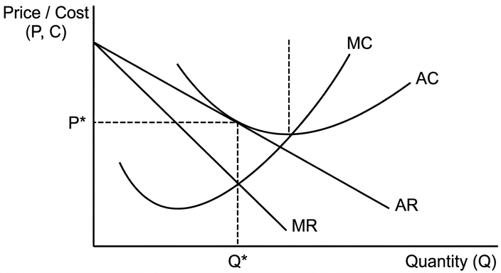
The diagram shows a firm in long-run equilibrium. The profit-maximising output is where MC = MR. At this output, the average revenue (AR) curve just touches the average cost (AC) curve, so AR = AC, meaning the firm earns normal profit (zero supernormal profit).
Monopolistic competition; normal profits in the long run.
Background Concept
Monopolistic competition is a market structure characterized by:
- Many firms.
- Differentiated products (each firm's product is slightly different from others).
- Free entry and exit in the long run.
- Each firm has some market power (downward-sloping demand curve) but faces competition.
In the short run, firms can earn supernormal profits. However, in the long run, the existence of supernormal profits attracts new firms entering the market, which shifts the demand curve for each existing firm leftward until only normal profits are earned. This is because the entry of new firms increases competition and reduces the market share of existing firms. In long-run equilibrium, the firm's demand curve is tangent to its average cost curve, so price equals average cost, and economic profit is zero.
Understanding the Question
The question has two parts: (1) Identify the probable market structure of the RMG industry in Bangladesh, (2) with the help of a diagram, consider the likely effect on the level of long-run profits of firms in this industry. The passage provides clues: over 4000 firms, differentiated by quality and speed of delivery, supplying many retailers. This strongly suggests monopolistic competition. The effect on long-run profits is that they will be normal due to free entry.
Approach
First, identify the market structure using the characteristics from the passage. Then draw a diagram showing the long-run equilibrium of a firm in monopolistic competition. Explain that in the long run, firms earn normal profits because entry eliminates supernormal profits. Make sure to label the diagram properly.
Step-by-Step Reasoning
- Identify market structure: Many firms (over 4000), differentiated products (quality, delivery speed), no evidence of barriers to entry. Therefore, monopolistic competition.
- Diagram:
- Axes: quantity (Q) on x-axis, price/cost (P, C) on y-axis.
- Downward-sloping demand curve (AR) and marginal revenue curve (MR) below it.
- U-shaped average cost (AC) and marginal cost (MC) curves.
- Profit-maximising output: where MC = MR (point Q*).
- At Q*, the price is determined from the demand curve (P*).
- In long-run equilibrium, the demand curve is tangent to the AC curve at Q*, so AR = AC at Q*. No supernormal profit.
- Explanation: Free entry shifts the demand curve leftward until it just touches the AC curve. At this point, total revenue equals total cost, so normal profit is earned.
- Conclusion: In the long run, firms in monopolistic competition earn normal profit only.
Key Takeaways
- Monopolistic competition leads to normal profits in the long run due to free entry.
- Product differentiation gives firms some market power but not enough to sustain supernormal profits.
- The diagram is crucial for demonstrating the tangency condition.
Common Mistakes
- Confusing monopolistic competition with monopoly or perfect competition.
- Drawing a diagram with supernormal profit in the long run (i.e., AR > AC at Q*).
- Forgetting to label axes and curves.
- Not explaining the diagram in words.
Things to Be Careful About
- The mark scheme allows up to 5 marks if the market is misidentified but analysis is correct. So even if you think it's something else, the analysis must be consistent.
- The diagram must show MC=MR and the tangency of AR and AC.
- The question asks to "consider" the effect on profits, so a brief explanation is enough.
With reference to the article, assess whether there is enough evidence to conclude that living standards in Bangladesh have improved since 1971.
Answer
Living standards include both monetary aspects (income, consumption) and non-monetary aspects (health, education, environment, working conditions).
Evidence of improvement in living standards:
- GNI per capita at constant prices rose from $2342 to $5823 between 2000 and 2020, a 143% increase.
- HDI rose from 0.49 to 0.66.
- Agricultural output increased by over 100% while employment fell, indicating rising productivity and potential for higher incomes.
- Net exports from the RMG sector stood at $23 billion, improving the balance of trade and allowing wider imports of goods and services.
Evidence of potential deterioration in living standards:
- Air and water pollution from the RMG industry (negative externalities) reduce quality of life.
- Use of child labour and poorly constructed factories indicate poor working conditions.
- Loss of agricultural jobs may have caused hardship for some workers.
Conclusion: The article provides some evidence of improved living standards, especially in terms of income and aggregate measures. However, key non-monetary indicators such as housing, health, education, and environmental quality are not fully addressed. The negative externalities and social costs mentioned suggest that the improvements may not have been evenly distributed or sustainable. Therefore, the evidence is insufficient to conclude that living standards have improved unambiguously.
The article provides some evidence of improvement but also significant drawbacks, and lacks comprehensive data, so the evidence is insufficient to conclude that living standards have improved unambiguously.
Background Concept
Living standards are a broad concept that includes both monetary and non-monetary aspects. Monetary indicators include income per capita (GDP, GNI) and consumption. Non-monetary indicators include health, education, environmental quality, housing, working conditions, and political freedom. Composite indicators like the HDI combine both. When assessing whether living standards have improved, it is important to consider both dimensions and weigh trade-offs. Negative externalities, such as pollution, can reduce well-being even if income rises.
Understanding the Question
The question asks to assess whether there is enough evidence in the article to conclude that living standards in Bangladesh have improved since 1971. The article provides data on GNI per capita, HDI, agricultural output, trade balance, employment shifts, and mentions negative externalities. You need to evaluate the evidence: what supports improvement, what suggests problems, and whether the evidence is sufficient to draw a firm conclusion. The command word "assess" requires a balanced argument and a justified conclusion.
Approach
First, define living standards as both monetary and non-monetary. Then present the evidence for improvement from the article: rising GNI, HDI, agricultural productivity, improved trade balance, wider imports. Then present the counter-evidence: pollution, child labour, poor working conditions, loss of agricultural jobs. Finally, evaluate whether the evidence is sufficient: note that the article lacks data on housing, health, education, and distribution of income. Conclude that while some improvements have occurred, the article does not provide enough comprehensive evidence to conclude that living standards have improved unambiguously.
Step-by-Step Reasoning
- Define living standards: include income (monetary) and factors like health, education, environment, working conditions.
- Evidence for improvement:
- GNI per capita doubled from $2342 to $5823 (real terms), a 143% increase.
- HDI rose from 0.49 to 0.66, indicating improvements in health, education, and income.
- Agricultural output more than doubled while employment fell, suggesting higher productivity and potential for higher incomes.
- Net exports from RMG sector were $23 billion, improving the balance of trade and allowing more imports.
- Wider range of goods and services imported.
- Evidence against improvement:
- Air and water pollution from chemicals used in cotton growing and manufacturing (negative externalities) reduce environmental quality.
- Use of child labour and poorly constructed factories indicate poor working conditions and potential exploitation.
- Loss of agricultural jobs may have led to unemployment or low-wage work.
- Assessment of sufficiency:
- The article provides some monetary and composite indicators but lacks details on health outcomes (e.g., infant mortality, life expectancy beyond HDI), education quality, housing, and income distribution.
- The negative externalities cited suggest that the growth may have come at social and environmental costs, which are not captured by GNI or HDI.
- The article does not provide data on poverty rates, inequality, or access to services.
- Therefore, while the evidence points to some improvements, it is insufficient to conclude that living standards have improved for all or that the improvements are sustainable.
- Conclusion: The article offers partial evidence but not enough to conclude that living standards have improved unambiguously. More comprehensive data on non-monetary indicators and distribution would be needed.
Key Takeaways
- Living standards are multi-dimensional.
- GNI per capita and HDI have limitations.
- Negative externalities must be considered.
- A conclusion must be justified based on the evidence provided.
Common Mistakes
- Only discussing improvements, ignoring drawbacks (one-sided answer loses marks).
- Not using data from the article to support points.
- Failing to reach a clear conclusion.
- Concluding that living standards have improved without acknowledging limitations of the evidence.
Things to Be Careful About
- The mark scheme explicitly mentions "Conclusion: Not enough evidence in the article" and "No information on housing/education or health". So the conclusion should reflect that the evidence is insufficient.
- Use specific figures from the article ($2342 to $5823, 0.49 to 0.66, etc.).
- The answer must be balanced: both improvements and disadvantages, then a conclusion.
With the help of a diagram, consider whether economic efficiency can be achieved without government intervention in a market economy.
Introduction
Economic efficiency comprises allocative efficiency (where price equals marginal cost, P = MC, ensuring resources are allocated to their most valued uses) and productive efficiency (where production occurs at minimum average cost, minimising waste). This essay considers whether a market economy can achieve these efficiencies without government intervention.
The case for the market achieving efficiency without intervention
Under perfect competition, the market mechanism can achieve both allocative and productive efficiency in the long run without any government intervention. Firms are price takers, and the market price is determined by industry demand and supply. Each firm faces a horizontal demand curve at the market price and maximises profit by producing where marginal cost equals marginal revenue (MC = MR = P). In the long run, free entry and exit ensure that firms earn only normal profit, and production occurs at the minimum point of the average cost curve.
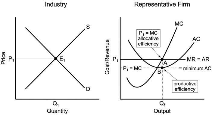
The diagram illustrates a perfectly competitive industry in long-run equilibrium. The left panel shows industry demand (D) and supply (S) intersecting at price P1 and quantity Q1. The right panel shows a representative firm facing a horizontal demand curve at price P1 (also its marginal revenue and average revenue). The firm produces output Qf where MC = MR = P1, and the average cost curve AC is at its minimum at this output. Thus, P1 = MC = minimum AC, satisfying both allocative efficiency (P = MC) and productive efficiency (production at minimum AC). This outcome arises spontaneously from the pursuit of self-interest, guided by the price mechanism, without any government intervention.
Therefore, under the ideal conditions of perfect competition, economic efficiency can be achieved without government intervention.
The case for government intervention being necessary
In reality, markets often fail to achieve efficiency due to various market failures. These include:
-
Externalities: Negative externalities, such as pollution, cause the social cost of production to exceed the private cost. Firms produce where MPC = MPB, but the socially optimal output is where MSC = MSB, leading to overproduction and a deadweight loss. Positive externalities, such as education, lead to underconsumption. Without intervention (e.g., taxes, subsidies), efficiency is lost.
-
Public goods: Pure public goods are non-rival and non-excludable, so the private sector underprovides them. Government provision is necessary to achieve efficiency.
-
Imperfect information: Consumers may lack information about the benefits of merit goods (e.g., healthcare) or the harms of demerit goods (e.g., tobacco), leading to under- or overconsumption. Government intervention (e.g., regulation, information provision) can improve outcomes.
-
Monopoly power: Monopolies restrict output and raise price above marginal cost, creating a deadweight loss and allocative inefficiency. Government regulation or competition policy may be needed.
-
Factor immobility: Occupational and geographical immobility of labour can lead to unemployment and productive inefficiency. Government training and relocation policies can help.
-
Inequity: Markets may produce an unequal distribution of income, which, while not strictly an efficiency issue, can lead to social exclusion and underinvestment in human capital, affecting long-run efficiency.
These market failures demonstrate that without government intervention, a market economy may not achieve economic efficiency.
Evaluation
The case for the market achieving efficiency without intervention relies on the strict assumptions of perfect competition: many buyers and sellers, homogeneous products, perfect information, no externalities, and perfect factor mobility. In reality, these assumptions are rarely met. However, government intervention is not a panacea. Government failure can occur due to imperfect information, regulatory capture, bureaucratic inefficiency, and unintended consequences. For example, a tax on a negative externality may be set at the wrong level, or a subsidy may create distortions. Moreover, intervention involves opportunity cost, as resources used for regulation could be used elsewhere.
Thus, the question is not whether intervention is always necessary, but whether the benefits of correcting a specific market failure outweigh the costs of government failure. In some cases, the market may self-correct (e.g., through Coasean bargaining if property rights are well-defined and transaction costs are low). In others, intervention is clearly beneficial (e.g., pollution taxes). The optimal approach often involves a mix of market mechanisms and carefully designed government policies.
Conclusion
Economic efficiency can be achieved without government intervention only under the ideal conditions of perfect competition and the absence of market failures. In practice, market failures are widespread, so some government intervention is typically required to improve efficiency. However, the extent and form of intervention must be carefully evaluated to avoid government failure. Therefore, while a purely free market can achieve efficiency in theory, in reality a combination of market forces and targeted government intervention is necessary to approach economic efficiency.
Economic efficiency can be achieved without government intervention only under the strict assumptions of perfect competition and no market failures; in reality, market failures necessitate some government intervention, but the extent depends on the specific context and the risk of government failure.
Background Concept
Economic efficiency is a central concept in microeconomics. It is typically divided into allocative efficiency and productive efficiency. Allocative efficiency occurs when resources are distributed such that the marginal benefit to society equals the marginal cost, i.e., price equals marginal cost (P = MC). This ensures that the mix of goods produced matches consumer preferences. Productive efficiency occurs when goods are produced at the lowest possible cost, i.e., at the minimum point of the average cost curve. Together, these conditions represent a Pareto optimal outcome where no one can be made better off without making someone else worse off.
Perfect competition is a market structure that, under ideal conditions, achieves both allocative and productive efficiency in long-run equilibrium. In perfect competition, there are many buyers and sellers, homogeneous products, perfect information, free entry and exit, and no externalities. Firms are price takers and produce where P = MC, and free entry ensures normal profit and production at minimum AC.
Market failures occur when the free market fails to allocate resources efficiently. Common market failures include externalities (where social costs or benefits diverge from private costs or benefits), public goods (non-rival and non-excludable, leading to underprovision), imperfect information (leading to under- or overconsumption of merit/demerit goods), monopoly power (leading to higher prices and lower output), and factor immobility (leading to unemployment and inefficiency). These failures provide a rationale for government intervention.
Government intervention can take many forms: taxes, subsidies, regulation, price controls, direct provision, information campaigns, and property rights. However, government intervention can also fail due to imperfect information, regulatory capture, bureaucratic inefficiency, and unintended consequences, known as government failure.
Understanding the Question
The question asks: "With the help of a diagram, consider whether economic efficiency can be achieved without government intervention in a market economy." The command word "consider" requires a balanced evaluation, presenting arguments for and against the proposition. The question also explicitly requires a diagram, which must be used to support the analysis. The diagram is not optional; without it, the maximum mark for AO1+AO2 is limited to Level 2 (6-10 marks).
The question is from Paper 4 and carries 20 marks, with 14 marks for AO1+AO2 (knowledge, understanding, and analysis) and 6 marks for AO3 (evaluation). The top band for AO1+AO2 requires detailed knowledge, fully developed explanations, accurate use of analytical tools (diagrams) that are fully explained, and a well-organised response. The top band for AO3 requires a justified conclusion that addresses the specific requirements of the question, with developed, reasoned, and well-supported evaluative comments.
Approach
To answer this question effectively, the following structure is recommended:
- Introduction: Define economic efficiency (allocative and productive) and outline the scope of the essay.
- The case for the market: Explain how a perfectly competitive market can achieve efficiency without intervention, using a diagram to illustrate the long-run equilibrium. This demonstrates the theoretical possibility.
- The case for government intervention: Discuss the main market failures that prevent efficiency, explaining each with a brief chain of reasoning. This shows why intervention may be necessary.
- Evaluation: Weigh the two sides. Consider the assumptions underlying the perfect competition model and the extent to which they hold in reality. Also consider the limitations of government intervention (government failure). Use criteria such as the severity of market failure, the effectiveness of intervention, and the opportunity cost.
- Conclusion: Provide a justified judgement that directly answers the question, stating the conditions under which efficiency can be achieved without intervention and the circumstances where intervention is needed.
The diagram should be placed in the section discussing perfect competition, as it directly supports the argument that efficiency can be achieved without intervention. The diagram must be fully explained in the text.
Step-by-Step Reasoning
Step 1: Define economic efficiency
Start by defining allocative efficiency (P = MC) and productive efficiency (minimum AC). This establishes the criteria against which the market's performance will be judged.
Step 2: Present the case for the market
Explain that under perfect competition, the market mechanism leads to efficiency. Describe the characteristics of perfect competition: many firms, price takers, free entry, perfect information. Explain the long-run equilibrium: firms produce where P = MC (allocative efficiency) and at the minimum of AC (productive efficiency). Use the diagram to illustrate.
Diagram explanation: The left panel shows the industry equilibrium where demand equals supply, determining the market price P1. The right panel shows a representative firm facing a horizontal demand curve at P1. The firm maximises profit by producing where MC = MR = P1, at output Qf. At this output, the AC curve is at its minimum, so P1 = MC = minimum AC. This demonstrates both allocative and productive efficiency. Emphasise that this outcome occurs without any government intervention; it is the result of the price mechanism and competition.
Step 3: Present the case for government intervention
Discuss the main market failures:
-
Externalities: Negative externalities (e.g., pollution) lead to overproduction because firms only consider private costs. The social cost (MSC) exceeds the private cost (MPC), so the market output is greater than the socially optimal output, creating a deadweight loss. Government intervention (e.g., a Pigouvian tax) can internalise the externality and restore efficiency. Positive externalities (e.g., education) lead to underconsumption; a subsidy can correct this.
-
Public goods: Pure public goods are non-rival and non-excludable, so private firms cannot profitably supply them. The market underprovides them, and government provision is necessary to achieve efficiency.
-
Imperfect information: Consumers may lack information about the true benefits or costs of goods. Merit goods (e.g., healthcare) are underconsumed; demerit goods (e.g., tobacco) are overconsumed. Government intervention (e.g., regulation, information campaigns) can improve outcomes.
-
Monopoly power: Monopolies restrict output and raise price above marginal cost, creating allocative inefficiency. Government competition policy or regulation can reduce this inefficiency.
-
Factor immobility: Labour immobility leads to unemployment and productive inefficiency. Government training and relocation policies can improve labour mobility and efficiency.
-
Inequity: While not strictly an efficiency issue, inequality can lead to social exclusion and underinvestment in human capital, affecting long-run efficiency. Redistributive policies can address this.
Each market failure should be explained with a clear chain of reasoning showing how it leads to inefficiency and how intervention can help.
Step 4: Evaluation
Now evaluate the two sides. The case for the market relies on the assumptions of perfect competition. In reality, these assumptions are rarely fully met. Most markets have some degree of imperfect competition, externalities, information asymmetries, etc. Therefore, in practice, some government intervention is usually needed to correct market failures.
However, government intervention is not always effective. Government failure can occur due to:
- Imperfect information: The government may not know the correct level of tax or subsidy.
- Regulatory capture: Regulators may act in the interests of the firms they regulate.
- Bureaucratic inefficiency: Government agencies may be wasteful.
- Unintended consequences: Policies may have side effects that reduce efficiency.
- Opportunity cost: Resources used for intervention could have been used elsewhere.
Thus, the net benefit of intervention depends on the specific context. In some cases, the market may self-correct (e.g., through Coasean bargaining if property rights are clear and transaction costs are low). In others, intervention is clearly beneficial (e.g., pollution taxes). The optimal approach often involves a mix of market mechanisms and carefully designed government policies.
Step 5: Conclusion
Reach a justified judgement. The conclusion should state that economic efficiency can be achieved without government intervention only under the ideal conditions of perfect competition and no market failures. In reality, market failures are widespread, so some government intervention is typically required to improve efficiency. However, the extent and form of intervention must be carefully evaluated to avoid government failure. Therefore, while a purely free market can achieve efficiency in theory, in reality a combination of market forces and targeted government intervention is necessary to approach economic efficiency.
Key Takeaways
- Economic efficiency has specific definitions: allocative efficiency (P = MC) and productive efficiency (minimum AC).
- Perfect competition is a theoretical benchmark where efficiency is achieved without intervention.
- Market failures (externalities, public goods, imperfect information, monopoly, factor immobility) provide reasons why real markets may not achieve efficiency.
- Government intervention can correct market failures but may also fail due to government failure.
- A balanced evaluation requires considering both market and government failures and reaching a context-specific judgement.
- A diagram is essential for this question; it must be fully explained.
Common Mistakes
- One-sided answer: Only arguing that markets fail or only that markets work. This loses all evaluation marks.
- No diagram or diagram not explained: The question explicitly requires a diagram; without it, the maximum mark is limited. Even with a diagram, if it is not explained in the text, it will not earn full marks.
- Confusing efficiency with equity: The question is about efficiency, not income distribution. While equity can affect efficiency indirectly, the focus should be on allocative and productive efficiency.
- Not reaching a justified conclusion: The top band for evaluation requires a justified conclusion. A summary of both sides without a clear judgement is insufficient.
- Listing many points without development: Depth of analysis is rewarded more than breadth. Develop a few key arguments fully rather than listing many shallow points.
- Using incorrect terminology: Ensure correct use of terms like allocative efficiency, productive efficiency, marginal cost, etc.
Things to Be Careful About
- Diagram: Label all axes and curves clearly. In the solution, explain what the diagram shows and how it supports the argument. Ensure the diagram is referenced in the text.
- Chain of reasoning: For each argument, build a clear causal chain. For example, for a negative externality: "Firms produce where MPC = MPB, but MSC > MPC, so the market output exceeds the socially optimal output, creating a deadweight loss. A tax equal to the external cost shifts the MPC curve upward, aligning private and social costs, and restoring efficiency."
- Evaluation criteria: Use specific criteria to weigh the arguments, such as the assumptions of perfect competition, the prevalence of market failures, the effectiveness of intervention, and the risk of government failure.
- Conclusion: Ensure the conclusion directly answers the question and is justified by the preceding analysis. Avoid fence-sitting without a clear verdict.
- Time management: In an exam, allocate time to plan the essay, draw the diagram, and write a coherent response. The essay should be well-organised and focused.
Evaluate whether the marginal revenue product theory (MRP) always explains the differences in wages.
Introduction
Marginal revenue product (MRP) theory states that the demand for labour is derived from the additional revenue a worker generates (MRP = MPP x MR). In a perfectly competitive labour market, the wage rate is determined by the interaction of demand (MRP) and supply of labour. This suggests that differences in wages across occupations and individuals can be explained by differences in MRP. This essay evaluates whether MRP theory always explains wage differences, or whether other factors such as market imperfections, institutional interventions, and discrimination play a significant role.
The Case for MRP Theory
In a perfectly competitive product and labour market, each firm is a wage taker and hires workers up to the point where MRP = wage. Therefore, differences in wages must reflect differences in MRP. MRP depends on the marginal physical product (MPP) of labour and the price of the product (MR). For example, workers in high-productivity industries (e.g., technology) generate higher MPP and higher product prices, so their MRP is higher, leading to higher wages. Additionally, non-wage factors such as education and training increase human capital and MPP, raising MRP. This explains wage differentials between skilled and unskilled workers. The theory also accounts for compensating differentials if working conditions affect supply, but the primary driver is demand-side MRP.
Limitations of MRP Theory
MRP theory assumes perfect competition: many firms, homogeneous labour, no trade unions, and perfect information. In reality, several factors prevent MRP from fully explaining wages:
- Imperfect competition in product markets: If a firm has market power, MR < price, so MRP is lower than the value of the marginal product. This could understate the contribution of labour, but still differences in MRP might reflect differences in monopoly power rather than productivity.
- Imperfect competition in labour markets: Monopsony employers (e.g., a single large firm in a town) can pay wages below MRP, so wages do not equal MRP. Differences in wages may then reflect differences in monopsony power rather than MRP.
- Trade unions: Unions can bargain for higher wages above the equilibrium MRP, especially in industries with strong union presence. This causes wage differences that are not explained by MRP.
- Government intervention: Minimum wage laws set a wage floor, compressing the wage distribution and preventing wages from falling to MRP for low-paid workers.
- Measurement problems: In many jobs (e.g., healthcare, education, collaborative work), it is difficult to isolate an individual worker's MRP. How can a teacher's MRP be measured? Wages may be set by non-market mechanisms such as public sector pay scales.
- Discrimination: Employers may pay different wages for equally productive workers based on gender, race, or other characteristics, violating MRP theory.
- Segmented labour markets: Primary and secondary labour markets may have different wage-setting mechanisms, with primary sector wages determined by internal labour markets rather than MRP.
Evaluation
MRP theory provides a powerful baseline explanation of wage differences: in competitive markets, wages tend to reflect productivity. However, the 'always' in the question is too strong. Real-world labour markets are riddled with imperfections that cause deviations from the MRP = wage condition. The extent to which MRP explains differences varies across contexts. In highly competitive sectors (e.g., gig economy, retail), MRP may be a good predictor. In regulated or unionised sectors, other factors dominate. Additionally, the difficulty of measuring MRP in many jobs means that wages are often set by convention, bargaining, or equity considerations. Nonetheless, the theory remains a useful starting point: any sustained difference in wages that cannot be explained by MRP tends to be corrected by market forces in the long run (e.g., worker mobility reduces wage gaps).
Conclusion
While MRP theory offers a logical explanation of wage differences based on productivity and demand, it does not always explain differences because of pervasive market imperfections, institutional factors, and measurement issues. A more complete explanation requires incorporating the roles of trade unions, government policy, discrimination, and market structure. Therefore, the answer to the question is that MRP theory does not always explain wage differences, but it remains a central concept in understanding the demand side of labour markets.
MRP theory does not always explain wage differences due to market imperfections, institutional factors, discrimination, and measurement difficulties, though it provides a useful baseline explanation.
Background Concept
Marginal revenue product (MRP) theory is a microeconomic theory of labour demand. It states that a profit-maximising firm will hire additional units of labour as long as the additional revenue generated by that worker (MRP) exceeds the wage. MRP is calculated as the marginal physical product of labour (MPP) multiplied by the marginal revenue from selling the output (MR). In a perfectly competitive product market, MR equals the price, so MRP = MPP x P. The demand curve for labour is the downward-sloping MRP curve (due to diminishing MPP). The supply of labour depends on factors such as population, preferences, and alternative wages. The equilibrium wage is determined where the demand for labour (MRP) equals the supply of labour. According to this theory, differences in wages across workers or occupations reflect differences in MRP, which in turn reflect differences in productivity (MPP) or the value of the output (MR).
Understanding the Question
The question asks: 'Evaluate whether the marginal revenue product theory (MRP) always explains the differences in wages.' The command word 'evaluate' requires a two-sided analysis and a justified conclusion. The word 'always' sets up an absolute claim, so the evaluation must challenge this absolute by identifying circumstances where MRP theory does not fully explain wage differences. The question is a 20-mark essay, so it requires a developed analysis of both the strengths and limitations of MRP theory in explaining wage differentials, and a final judgement. The top band for AO3 (evaluation) requires a justified conclusion that addresses the specific requirements of the question.
Approach
- Start by defining MRP theory and explaining how it predicts wage differences in a competitive market.
- Present the first side: the case for MRP theory as a strong explanation of wage differences. Use a diagram to illustrate two different labour markets (e.g., high-skill and low-skill) showing different MRP curves leading to different wages.
- Present the second side: limitations of MRP theory. Discuss market imperfections (monopoly, monopsony), trade unions, government intervention, measurement problems, discrimination, and segmented labour markets.
- Evaluate the strength of these limitations: some are more significant than others, and the extent to which MRP theory holds depends on the context.
- Conclude with a justified judgement: MRP theory does not always explain differences, but it provides a useful starting point.
Step-by-Step Reasoning
Step 1: Define MRP theory and its relevance to wage differences.
- MRP theory: demand for labour is derived from the MRP. In perfect competition, equilibrium wage = MRP. Therefore, differences in wages must come from differences in MRP, which depend on MPP and MR.
- Example: A surgeon has high MPP (saves many lives) and high MR (high fees), so high MRP leads to high wage. A cleaner has low MPP and low MR, so low wage.
Step 2: Explain the diagram.
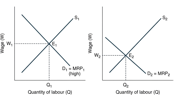
- Diagram 1: Two labour markets side by side. Left: high-MRP labour market (e.g., skilled workers). Demand curve D1 = MRP1, supply S1, equilibrium wage W1 and employment Q1. Right: low-MRP labour market (e.g., unskilled workers). Demand curve D2 = MRP2 (lower), supply S2, equilibrium wage W2 (lower) and employment Q2. This shows that differences in MRP lead to different wages.
Step 3: Develop the case for MRP theory.
- Differences in human capital (education, training) increase MPP, raising MRP and wages. This explains the skill premium.
- Differences in product demand affect MR (price). Workers in high-demand industries (e.g., tech) earn more.
- Compensating differentials for dangerous or unpleasant jobs can be incorporated through supply factors, but the demand side (MRP) remains central.
Step 4: Present limitations.
- Imperfect competition in product markets: If a firm has monopoly power, MR < price, so MRP is lower than the value of marginal product. Wages might be lower than in a competitive industry, even if productivity is the same. Wage differences may reflect market power, not just MRP.
- Imperfect competition in labour markets: Monopsony employers can pay wages below MRP. Example: a company town with one employer can set wages below MRP, creating wage differences that are not explained by MRP.
- Trade unions: Unions can raise wages above MRP through collective bargaining, especially in industries with strong unions (e.g., manufacturing). This creates wage differences that cannot be explained by MRP alone.
- Government intervention: Minimum wage laws set a wage floor, causing wages for low-skilled workers to be above their MRP. This reduces wage differences between low-skilled and some middle-skilled workers.
- Measurement problems: In many jobs (e.g., teachers, nurses, collaborative work), it is impossible to measure individual MRP. Wages are set by public sector pay scales, negotiation, or tradition, not by MRP.
- Discrimination: Employers may pay women less than men for the same work, even if MRP is equal. This is a violation of MRP theory and can cause wage differences unrelated to productivity.
- Segmented labour markets: The primary sector (e.g., large firms with internal labour markets) may have wages determined by seniority and job ladders, not MRP. The secondary sector (e.g., small firms, temporary work) may have wages closer to MRP. Differences between sectors may not reflect MRP.
Step 5: Evaluation.
- Weigh the strengths and weaknesses: MRP theory is a powerful baseline, but it assumes perfect competition. In reality, market imperfections are widespread. The extent to which MRP explains differences varies: in highly competitive labour markets (e.g., freelance, gig economy), MRP is a good predictor; in regulated or unionised markets, it is less so.
- Consider the long run: market forces tend to correct deviations (e.g., workers move to higher-paying jobs, reducing wage gaps), but this is slow and imperfect.
- The question asks 'always' – the absolute claim is too strong. Even in the most competitive markets, there are frictions and measurement issues. Therefore, MRP theory does not always explain differences.
Step 6: Conclusion.
- Justified conclusion: MRP theory is a key determinant of wages, but it is not the sole explanation. Other factors such as monopsony power, trade unions, government policy, discrimination, and measurement difficulties mean that wage differences are not always explained by MRP. A more comprehensive theory is needed.
Key Takeaways
- MRP theory links wages to productivity and is a core concept in labour economics.
- The theory works best under perfect competition; deviations occur in real markets.
- Wage differences arise from a combination of demand-side (MRP) and supply-side factors, as well as institutional and market imperfections.
- Evaluation requires challenging the absolute claim ('always') and providing a balanced judgement.
Common Mistakes
- One-sided answers: writing only about MRP theory or only about its limitations. This loses AO3 marks.
- No conclusion or a vague conclusion: top band for AO3 requires a justified conclusion that addresses the specific question.
- Ignoring the 'always' aspect: failing to discuss whether MRP theory is a complete explanation.
- Overstating the case for MRP theory without acknowledging real-world complexities.
- Not using the diagram: while not required, a diagram can strengthen the analysis and demonstrate understanding.
Things to Be Careful About
- Ensure the diagram is clearly explained in the text. The diagram should show two different MRP curves to illustrate wage differences.
- Use precise terminology: MRP, MPP, marginal revenue, perfect competition, monopsony, discrimination.
- Distinguish between the demand for labour (MRP) and the supply of labour; both determine wages, but the question focuses on MRP as the demand-side explanation.
- Avoid making the essay too descriptive; the analysis should be developed and evaluative.
- The conclusion should be specific: 'not always' rather than 'it depends' without elaboration.
A country with an open economy has falling demand for exports.
Consider the view that monetary policy alone will solve this problem.
Introduction
An open economy is one that engages in international trade, so aggregate demand (AD) includes net exports (X – M). Falling demand for exports directly reduces AD, causing a contractionary gap. The view that monetary policy alone can solve this problem rests on its ability to depreciate the exchange rate and boost net exports. However, the effectiveness of such a policy depends on elasticities, time lags, and potential conflicts with other macroeconomic objectives.
The case for monetary policy
Expansionary monetary policy – lowering the policy interest rate – works through two channels. First, lower interest rates reduce the return on domestic assets, causing capital outflows and a depreciation of the exchange rate. A weaker currency makes exports cheaper in foreign currency and imports dearer, so net exports rise. Second, lower interest rates stimulate domestic consumption and investment, further increasing AD. The combined effect can offset the initial fall in exports.
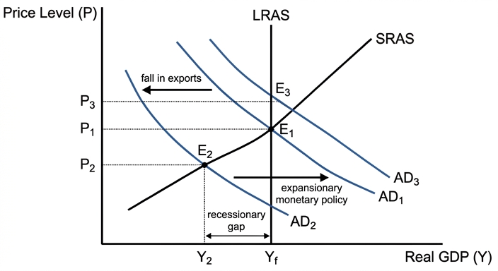
In the diagram, the economy is initially at full employment (Yf) with price level P1. The fall in export demand shifts AD leftwards from AD1 to AD2, creating a recessionary gap. Expansionary monetary policy shifts AD rightwards from AD2 to AD3, restoring Yf. If the Marshall-Lerner condition holds (the sum of the price elasticities of demand for exports and imports exceeds one), the depreciation will improve the trade balance in the long run. Thus, in theory, monetary policy alone can restore output and employment.
The case against monetary policy
Several factors limit the effectiveness of monetary policy alone. First, the J-curve effect means that in the short run, the trade balance may worsen because contracts are fixed and volumes adjust slowly. Second, if the demand for exports is price-inelastic, depreciation will not significantly raise export revenue. Third, expansionary monetary policy may conflict with other objectives: it can fuel inflation (shifting AD rightwards when the economy is already near capacity) and may cause a depreciation that increases the cost of imported inputs, worsening cost-push inflation. Fourth, the problem may be structural – falling export demand due to loss of comparative advantage or poor product quality – which monetary policy cannot address. Supply-side policies (e.g., subsidies, innovation support) would be more appropriate.
Evaluation
The effectiveness of monetary policy alone depends on the elasticity of demand for exports, the state of the economy, and the time horizon. If the economy has spare capacity and the Marshall-Lerner condition holds, monetary policy can be effective in the medium term. However, if the economy is at full employment, the policy may cause inflation without raising output. Moreover, if the fall in exports is due to structural factors, monetary policy is a temporary fix. A combination of monetary policy to manage the exchange rate and supply-side policies to improve competitiveness is likely to be more sustainable.
Conclusion
Monetary policy alone can solve the problem of falling export demand only under specific conditions: spare capacity, elastic demand for exports, and a willingness to accept a temporary depreciation and possible inflation. In many real-world contexts, structural issues and policy conflicts mean that monetary policy is insufficient on its own. Therefore, the view that monetary policy alone will solve the problem is too simplistic; a broader policy mix is usually required.
Monetary policy alone can solve falling export demand only under favourable conditions (spare capacity, elastic demand, Marshall-Lerner condition satisfied); in practice, structural factors and policy conflicts usually require a mix of monetary and supply-side policies.
Background Concept
This question tests understanding of open-economy macroeconomics, specifically how a fall in export demand affects aggregate demand and how monetary policy can influence the exchange rate and net exports. Key concepts include:
- Aggregate demand (AD) = C + I + G + (X – M). A fall in exports directly reduces AD.
- Monetary policy transmission: lower interest rates -> capital outflows -> depreciation -> net exports rise (if Marshall-Lerner condition holds). Also lower rates stimulate domestic spending.
- The Marshall-Lerner condition: a depreciation improves the trade balance if the sum of the price elasticities of demand for exports and imports is greater than one.
- The J-curve effect: in the short run, the trade balance may worsen after depreciation because volumes adjust slowly; improvement comes later.
- Policy conflicts: expansionary monetary policy can cause inflation, especially if the economy is at full employment.
- Supply-side policies: address structural issues like competitiveness, productivity, and product quality.
Understanding the Question
The question presents a scenario: an open economy faces falling demand for exports. The statement to evaluate is that "monetary policy alone will solve this problem." The command word "Consider" implies evaluation – you must discuss both the potential effectiveness of monetary policy and its limitations, then reach a justified conclusion. The top band requires detailed knowledge, fully developed analysis, accurate use of analytical tools (diagrams), and a justified conclusion. The question does not specify a diagram, but using one (e.g., AD/AS) strengthens the analysis and helps achieve the top band.
Approach
- Define an open economy and explain how falling exports reduce AD.
- Explain the theoretical case for monetary policy: lower interest rates -> depreciation -> higher net exports -> AD recovers. Use an AD/AS diagram to illustrate.
- Develop the counter-argument: limitations including the J-curve, inelastic demand, inflation risk, structural causes, and policy conflicts.
- Evaluate by weighing the conditions under which monetary policy works (spare capacity, elastic demand) against those where it fails (full employment, structural decline).
- Conclude with a justified judgement: monetary policy alone is insufficient in most real-world situations; a policy mix is better.
Step-by-Step Reasoning
Step 1: The initial impact
Falling export demand reduces net exports (X – M). In the AD/AS model, this shifts AD leftwards. If the economy was at full employment, a recessionary gap opens – output falls below potential, unemployment rises. The problem is a demand-side shock.
Step 2: How monetary policy can help
The central bank can lower the policy interest rate. This reduces the return on domestic assets, leading to capital outflows and a depreciation of the exchange rate. A weaker currency makes exports cheaper abroad and imports more expensive at home. If the Marshall-Lerner condition holds, the trade balance improves in the medium term. Additionally, lower interest rates stimulate consumption and investment, further boosting AD. The AD curve shifts rightwards, potentially closing the recessionary gap.
Step 3: The diagram
Draw an AD/AS diagram with LRAS vertical at Yf, SRAS upward sloping, and AD1 intersecting at Yf, P1. A leftward shift to AD2 creates a recessionary gap (Y2 < Yf). Expansionary monetary policy shifts AD rightwards to AD3, restoring Yf but at a higher price level P3. This shows that monetary policy can restore output but may cause inflation.
Step 4: Limitations
- J-curve effect: In the short run, the trade balance may worsen because existing contracts are in place and volumes take time to adjust. The improvement occurs only after several months or years.
- Elasticity conditions: If export demand is price-inelastic (e.g., primary commodities), depreciation may not significantly increase export revenue. The Marshall-Lerner condition may not hold.
- Inflation: If the economy is at full employment, the increase in AD from monetary policy will mainly raise prices rather than output, causing demand-pull inflation. Also, depreciation raises import prices, contributing to cost-push inflation.
- Structural issues: Falling exports may be due to poor product quality, lack of innovation, or loss of comparative advantage. Monetary policy cannot fix these; supply-side policies (e.g., R&D subsidies, education, infrastructure) are needed.
- Policy conflicts: Expansionary monetary policy may conflict with an inflation target. Also, if the government is also using fiscal policy, there may be crowding out or coordination issues.
Step 5: Evaluation
Weigh the conditions: monetary policy is most effective when there is spare capacity (so inflation is not a major concern), when export demand is elastic, and when the problem is cyclical rather than structural. In many developing economies, exports are often primary commodities with low price elasticity, so depreciation may not help much. Also, the J-curve means that in the short run, the problem may worsen before it improves. Therefore, while monetary policy can be part of the solution, relying on it alone is risky. A combination with supply-side policies to improve competitiveness and diversify exports is more robust.
Step 6: Conclusion
The view that monetary policy alone will solve the problem is too simplistic. It can work under specific conditions, but in practice, structural factors and policy trade-offs mean that a broader approach is usually required. The conclusion should state this clearly, justifying why.
Key Takeaways
- Understand the transmission mechanism of monetary policy in an open economy: interest rates -> exchange rate -> net exports.
- Know the Marshall-Lerner condition and J-curve effect and how they qualify the effectiveness of depreciation.
- Be able to use AD/AS diagrams to illustrate demand shocks and policy responses.
- Recognise that policy effectiveness depends on context (elasticities, capacity, time horizon).
- For evaluative questions, always present both sides and reach a justified conclusion.
Common Mistakes
- Writing a one-sided answer that only explains how monetary policy works, without discussing limitations. This loses all evaluation marks (AO3).
- Failing to include a diagram when it would strengthen the analysis. While not mandatory, a diagram helps achieve the top band.
- Ignoring the J-curve and Marshall-Lerner condition – these are key evaluative points.
- Concluding without a clear judgement, e.g., "it depends" without saying on what and which way.
- Confusing monetary policy with fiscal policy or exchange rate policy (direct devaluation is not monetary policy; monetary policy can influence the exchange rate indirectly).
- Not linking the analysis to the specific problem of falling exports – generic answers about monetary policy lose focus.
Things to Be Careful About
- Clearly distinguish between direct devaluation (fiscal/exchange rate policy) and monetary policy-induced depreciation.
- Label axes and curves in the diagram: price level on vertical axis, real GDP on horizontal; AD, SRAS, LRAS; show shifts and new equilibrium points.
- Use the extract's context: the country has an open economy, so the exchange rate channel is relevant.
- In the conclusion, state the extent to which monetary policy alone can solve the problem, not just list pros and cons.
- Keep the analysis focused on the question: is monetary policy alone sufficient? Not whether it is useful at all.
- Use correct economic terminology: recessionary gap, transmission mechanism, depreciation, elasticity, etc.
Evaluate how a country might increase its potential economic growth.
Introduction
Potential economic growth refers to the long-run expansion of an economy's productive capacity, shown by an outward shift of the LRAS curve or the production possibility curve (PPC). It is determined by the quantity and quality of factors of production and the efficiency with which they are combined. A country can increase its potential growth through supply-side policies that raise the stock of capital, improve labour productivity, and enhance technological progress.
Supply-side policies to increase potential growth
Investment in education and training raises the human capital of the labour force. Better-educated workers are more productive, which shifts the LRAS curve to the right. For example, government spending on vocational training and higher education increases the marginal product of labour, enabling the economy to produce more output from the same quantity of workers. This also improves occupational mobility, reducing structural unemployment and further expanding the effective labour supply.
Investment in infrastructure and R&D increases the capital stock and fosters innovation. Improved transport networks reduce production costs and enable economies of scale, while R&D leads to new technologies that raise total factor productivity. The resulting outward shift of the PPC represents a permanent increase in the economy's capacity to produce goods and services.
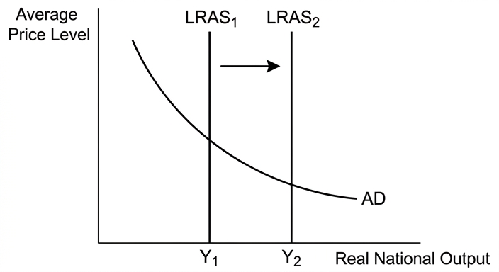
The diagram shows the LRAS curve shifting from LRAS1 to LRAS2, representing an increase in potential output from Y1 to Y2. In the AD/AS framework, this allows the economy to achieve a higher real national output without generating demand-pull inflation. On a PPC, the curve shifts outward from PPC1 to PPC2, indicating a greater maximum combination of goods the economy can produce.
Pro-competition policies and deregulation increase efficiency by reducing barriers to entry and encouraging rivalry. In contestable markets, firms are forced to minimise costs and innovate, which improves both productive and dynamic efficiency. Privatisation of state-owned enterprises can also improve efficiency if the firms are exposed to market discipline, though this depends on the regulatory framework.
Labour market reforms such as reducing the power of trade unions or lowering the national minimum wage can increase labour market flexibility, making it easier for firms to hire workers and adjust wages. This can raise the employment rate and the natural rate of output, though the effect on productivity is ambiguous.
Evaluation
Supply-side policies face significant constraints. First, time lags are substantial: education and R&D take years or decades to feed through into higher productivity. Governments with short electoral cycles may prioritise policies with quicker payoffs, such as tax cuts, which may boost demand but not potential supply.
Second, government finance is a binding constraint. Investment in infrastructure and education requires large public spending, which may increase government borrowing. If borrowing raises interest rates, it can crowd out private investment, offsetting some of the supply-side gains. In developing countries, limited tax revenue and access to credit may make such investment infeasible.
Third, political constraints can undermine reforms. Privatisation may be opposed by trade unions or the public, and deregulation may face resistance from incumbent firms. Labour market reforms that reduce worker protections may be politically unpopular and could increase inequality, which may itself harm long-run growth by reducing social cohesion.
Fourth, the environmental impact of increased production must be considered. Unchecked growth may deplete natural resources and cause pollution, which reduces sustainable growth. Policies that promote green technology and resource efficiency can mitigate this, but they add to the cost.
Conclusion
A country can increase its potential economic growth most effectively through a coordinated package of supply-side policies, particularly investment in human capital and infrastructure, combined with pro-competition measures. However, the effectiveness of these policies is limited by time lags, fiscal constraints, and political feasibility. For a developing country, the binding constraint is often the shortage of finance and institutional capacity, making foreign direct investment and aid important complements. In the long run, the most sustainable route is investment in education and R&D, which raises both the quantity and quality of factors of production without the environmental costs of pure capital accumulation.
A country can increase its potential economic growth most effectively through a coordinated package of supply-side policies, particularly investment in human capital and infrastructure combined with pro-competition measures, but the effectiveness is constrained by time lags, fiscal limitations, and political feasibility; the most sustainable route is investment in education and R&D.
Background Concept
Potential economic growth is the increase in the economy's productive capacity over the long run. It is distinct from actual growth, which can fluctuate with the business cycle. Potential growth is determined by the quantity and quality of factors of production (labour, capital, land, and entrepreneurship) and the efficiency with which they are combined. It is represented by an outward shift of the long-run aggregate supply (LRAS) curve or the production possibility curve (PPC).
Supply-side policies are government measures designed to increase the productive capacity of the economy. They can be market-based (deregulation, privatisation, tax reforms) or interventionist (government spending on education, infrastructure, R&D). The key is that they shift LRAS to the right, allowing the economy to produce more output at the same price level.
Understanding the Question
The question asks you to 'evaluate how a country might increase its potential economic growth.' This is a 20-mark undivided essay (2023 onwards format) with AO1+AO2 out of 14 and AO3 out of 6. The command word 'evaluate' requires you to present both sides: the case for how policies can increase potential growth, and the constraints or limitations that reduce their effectiveness. You must reach a justified conclusion that addresses the specific question.
The top band for AO1/AO2 demands detailed knowledge, fully developed explanations, accurate use of analytical tools (diagrams), and a well-organised response. The top band for AO3 demands a justified conclusion with developed, reasoned evaluative comments.
Approach
- Define potential economic growth and explain how it is measured (LRAS, PPC).
- Identify and analyse at least two supply-side policies that can increase potential growth. For each, build a developed chain of reasoning showing how the policy shifts LRAS.
- Include a diagram (LRAS shift or PPC shift) and explain it fully.
- Evaluate the policies against constraints: time lags, government finance, political feasibility, environmental impact, and potential trade-offs.
- Conclude with a justified judgement on the most effective approach, considering the country's context.
Step-by-Step Reasoning
Step 1: Define potential economic growth
Potential economic growth is the long-run expansion of the economy's productive capacity. It is shown by an outward shift of the LRAS curve or the PPC. It depends on the quantity and quality of factors of production and the efficiency of their use.
Step 2: Analyse supply-side policies
Policy 1: Investment in education and training
- Government spending on schools, universities, and vocational training increases the human capital of the labour force.
- A more educated workforce is more productive: each worker can produce more output per hour (higher marginal product of labour).
- This shifts the LRAS curve to the right because the economy can produce more output at every price level.
- It also improves occupational mobility, reducing structural unemployment and increasing the effective labour supply.
- Example: South Korea's heavy investment in education from the 1960s onwards is widely credited with its rapid potential growth.
Policy 2: Investment in infrastructure and R&D
- Infrastructure (roads, ports, digital networks) reduces production costs and enables economies of scale.
- R&D leads to new technologies and processes that raise total factor productivity.
- Both increase the capital stock and improve its quality, shifting LRAS right.
- Example: The UK's investment in high-speed rail (HS2) aims to reduce travel times and boost productivity in connected regions.
Policy 3: Pro-competition policies and deregulation
- Reducing barriers to entry and encouraging competition forces firms to minimise costs and innovate.
- This improves productive efficiency (firms produce at minimum AC) and dynamic efficiency (innovation over time).
- Privatisation can improve efficiency if state-owned firms are exposed to market discipline, but this depends on effective regulation.
Policy 4: Labour market reforms
- Reducing trade union power or lowering minimum wages can increase labour market flexibility.
- Firms can hire more easily and adjust wages to market conditions, potentially raising employment and output.
- However, the effect on productivity is ambiguous: lower wages may reduce worker motivation and investment in training.
Step 3: Diagram
The diagram shows the LRAS curve shifting from LRAS1 to LRAS2. The vertical axis is the average price level, and the horizontal axis is real national output. The shift indicates that the economy can now produce a higher potential output (Y2 > Y1) at the same price level. Alternatively, a PPC diagram shows the curve shifting outward from PPC1 to PPC2, representing a greater maximum combination of goods.
Step 4: Evaluation
Time lags: Education and R&D take years or decades to affect potential output. Governments with short electoral cycles may prefer demand-side policies with quicker results, even if they do not increase potential growth.
Government finance: Investment in infrastructure and education requires large public spending. If the government borrows to finance this, it may raise interest rates and crowd out private investment. In developing countries, limited tax revenue and access to credit may make such investment impossible without foreign aid or FDI.
Political constraints: Privatisation and deregulation may face opposition from trade unions, incumbent firms, or the public. Labour market reforms that reduce worker protections may be politically unpopular and could increase inequality, which may itself harm long-run growth by reducing social cohesion and human capital formation.
Environmental impact: Increased production may deplete natural resources and cause pollution, reducing sustainable growth. Policies that promote green technology and resource efficiency can mitigate this, but they add to the cost and may reduce the short-run increase in output.
Trade-offs: Some policies may conflict with other macroeconomic objectives. For example, reducing the minimum wage may increase employment but worsen income inequality. Deregulation may boost growth but increase financial instability.
Step 5: Conclusion
The most effective approach is a coordinated package of supply-side policies, with a focus on investment in human capital and infrastructure. These have the largest and most sustainable impact on potential growth. However, the effectiveness depends on the country's context: for a developed country, the main constraints are political feasibility and time lags; for a developing country, the binding constraint is often the shortage of finance and institutional capacity, making FDI and aid important complements. In the long run, investment in education and R&D is the most sustainable route because it raises both the quantity and quality of factors of production without the environmental costs of pure capital accumulation.
Key Takeaways
- Potential economic growth is about expanding the economy's productive capacity, not just boosting demand.
- Supply-side policies are the main tools, but they take time and require careful implementation.
- Evaluation must consider constraints: time lags, government finance, political feasibility, and environmental impact.
- A justified conclusion weighs the trade-offs and reaches a verdict specific to the question.
Common Mistakes
- Confusing potential growth with actual growth: many students write about demand-side policies (fiscal/monetary) to boost actual growth, which does not increase potential growth.
- Listing many policies without developing any: the top band requires detailed analysis of at least two policies, not a superficial list of five.
- Omitting the diagram or not explaining it: the mark scheme caps at Level 2 if no diagram is included or if it is not explained.
- One-sided evaluation: the question asks for evaluation, so you must discuss both the strengths and limitations of the policies.
- No conclusion or a vague conclusion: the top band for AO3 requires a justified conclusion that addresses the specific question.
Things to Be Careful About
- Label the diagram clearly: axes (price level and real output for LRAS; capital goods and consumer goods for PPC), curves (LRAS1, LRAS2; PPC1, PPC2), and the direction of the shift.
- Explain the diagram in the text: state what the shift represents and why it occurs.
- Use specific examples to support your analysis (e.g., South Korea's education investment, UK's HS2).
- Distinguish between market-based and interventionist supply-side policies.
- In the evaluation, avoid simply listing criticisms; develop each point and explain why it matters for the effectiveness of the policy.