Economics 9708/43 — May/June 2025
Cambridge A-Level · A Level Data Response and Essays · worked solutions for every part, with the mark scheme
Topics Effectiveness of Macroeconomic Policies · Employment and Unemployment · Economic Growth and Sustainability · Indifference Curves and Budget Lines · Growth and Survival of Firms · Costs of Production · +2 more
The influence of governments
People often talk as if governments can easily control economic outcomes.
Content removed due to copyright restrictions.
High-income countries decided to focus on economic growth realising that it was essential to generate revenues and taxes needed to pay for costly investments, for example, the storage of renewable energy, required to reduce the use of fossil fuels.
Sources: Irwin Stelzer, The Sunday Times, 29 January 2023
Ray Bourne, The Times, 9 February 2023
The article refers to structural unemployment. Explain what this means and whether it is the same as the natural rate of unemployment.
Answer
Structural unemployment occurs when there is a mismatch between the skills of the labour force and the skills required for available jobs, or when the number of jobs is insufficient relative to the number of job seekers due to structural changes in the economy. The natural rate of unemployment includes both structural unemployment and frictional unemployment. Therefore, they are not the same; the natural rate is a broader concept that encompasses structural unemployment along with frictional unemployment.
Structural unemployment is a type of unemployment caused by mismatches in the labour market, while the natural rate of unemployment includes both structural and frictional unemployment, so they are not the same.
Background Concept
Unemployment can be classified into different types: frictional, structural, cyclical, and seasonal. Structural unemployment arises from long-term changes in the economy, such as technological change or shifts in consumer demand, leading to a mismatch between workers' skills and job vacancies. The natural rate of unemployment is the rate of unemployment that exists when the economy is at full employment, consisting of frictional and structural unemployment. It does not include cyclical unemployment.
Understanding the Question
The question asks to explain structural unemployment and then determine whether it is the same as the natural rate of unemployment. This requires a clear definition of both terms and an understanding of their relationship.
Approach
First, define structural unemployment precisely. Then define the natural rate of unemployment. Finally, compare them, noting that the natural rate includes structural unemployment as a component, so they are not identical.
Step-by-Step Reasoning
- Structural unemployment: This occurs when the skills of workers do not match the skills demanded by employers, often due to technological change, changes in consumer preferences, or geographical immobility. For example, the decline of coal mining leads to unemployment among miners who lack skills for new industries.
- Natural rate of unemployment: This is the unemployment rate that prevails when the labour market is in equilibrium, with no cyclical unemployment. It consists of frictional unemployment (workers temporarily between jobs) and structural unemployment.
- Comparison: Since the natural rate includes structural unemployment, they are not the same. Structural unemployment is a subset of the natural rate. The natural rate is a broader concept that also includes frictional unemployment.
Key Takeaways
- Structural unemployment is a type of unemployment caused by mismatches in the labour market.
- The natural rate of unemployment is the sum of frictional and structural unemployment.
- Understanding the distinction helps in designing appropriate policies: structural unemployment requires retraining or education, while frictional unemployment may be reduced by improving information flows.
Common Mistakes
- Confusing structural unemployment with cyclical unemployment. Cyclical unemployment is due to a lack of aggregate demand, while structural is due to mismatches.
- Stating that the natural rate is the same as structural unemployment. The natural rate includes frictional as well.
Things to Be Careful About
- Be precise in definitions. The natural rate is not a fixed number; it can change over time due to changes in the structure of the economy.
- Use correct terminology: "structural unemployment" and "natural rate of unemployment".
To keep unemployment low, one government used fiscal policy. Analyse how this policy can affect unemployment rates.
Answer
Fiscal policy involves the use of government spending and taxation to influence the economy. To reduce unemployment, a government can adopt expansionary fiscal policy: increasing government spending or cutting taxes. This increases aggregate demand (AD). In the AD/AS diagram, AD shifts right from AD1 to AD2. Assuming the economy is operating below full capacity, real GDP rises from Y1 to Y2, and the price level rises from P1 to P2. The increase in output leads to higher demand for labour, reducing unemployment. The multiplier effect amplifies the initial increase in spending, as higher income leads to further consumption. For example, increased government spending on infrastructure creates jobs directly and indirectly through supply chains. Tax cuts increase disposable income, boosting consumption and AD. Thus, expansionary fiscal policy can effectively lower unemployment in the short run when there is spare capacity.
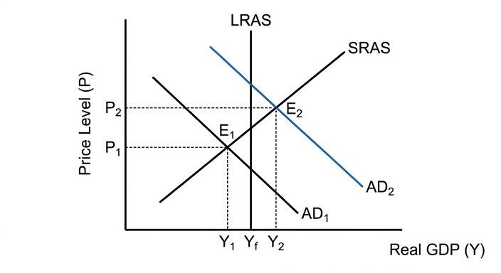
Expansionary fiscal policy increases aggregate demand, which raises output and reduces unemployment, especially when there is spare capacity.
Background Concept
Fiscal policy is a demand-side policy. Expansionary fiscal policy increases AD, which in a recessionary gap (below full employment) raises output and employment. The multiplier effect means that an initial injection of spending leads to a larger final increase in national income. However, if the economy is at full capacity, expansionary fiscal policy may cause inflation without reducing unemployment.
Understanding the Question
The question asks to analyse how fiscal policy can affect unemployment rates. It requires an explanation of the mechanism, including the role of the multiplier and the conditions under which it is effective. The marking scheme awards marks for defining fiscal policy, using a diagram, and explaining the effect on output and unemployment.
Approach
Start by defining fiscal policy. Then describe expansionary fiscal policy. Use an AD/AS diagram to illustrate the shift in AD and the resulting increase in output and decrease in unemployment. Explain the multiplier effect. Mention that the effectiveness depends on the state of the economy (spare capacity).
Step-by-Step Reasoning
- Definition: Fiscal policy is the use of government spending (G) and taxation (T) to influence aggregate demand.
- Expansionary fiscal policy: Increase G or decrease T. This directly increases AD (G is a component of AD; lower T increases disposable income and consumption).
- Diagram: Draw an AD/AS diagram with LRAS vertical, SRAS upward sloping, and AD downward sloping. Initial equilibrium at E1 with price level P1 and real GDP Y1, below full employment (Yf). Expansionary fiscal policy shifts AD to AD2. New equilibrium at E2 with higher real GDP Y2 and higher price level P2. The increase in output from Y1 to Y2 reduces unemployment because firms hire more workers to produce the higher output.
- Multiplier effect: The initial increase in spending leads to rounds of increased consumption, so the total increase in AD is larger than the initial injection. This amplifies the impact on output and employment.
- Examples: Government spending on infrastructure creates jobs directly and indirectly. Tax cuts increase consumer spending, boosting demand for goods and services, leading to more hiring.
- Limitations: If the economy is at full employment, expansionary fiscal policy may only cause inflation. Also, crowding out (higher interest rates reducing private investment) can offset some of the effect.
Key Takeaways
- Fiscal policy can reduce unemployment by increasing AD.
- The multiplier effect enhances the impact.
- The effectiveness depends on the economic context (spare capacity, crowding out).
Common Mistakes
- Forgetting to include the diagram or not explaining it.
- Not mentioning the multiplier.
- Assuming fiscal policy always works; ignoring potential crowding out or time lags.
Things to Be Careful About
- Label axes and curves correctly on the diagram.
- Explain the shift and the new equilibrium.
- Use the correct terminology: "expansionary fiscal policy", "aggregate demand", "multiplier".
Explain how the policies of high-income economies towards 'green energy' changed between 2015 and 2022.
Answer
Initially, at the Paris Agreement in 2015, high-income economies committed to increasing green energy outputs and reducing the use of fossil fuels in energy production. However, by 2022, these economies shifted their focus towards economic growth, allowing a continuation of energy production using fossil fuels. Additionally, the promised funds from rich to poor countries to support green energy transitions did not materialise, and poor countries were less effective in reducing CO2 emissions.
High-income economies shifted from a strong commitment to green energy (Paris Agreement) to a focus on economic growth and continued fossil fuel use by 2022, with promised funds not materialising.
Background Concept
Government policies towards green energy are influenced by multiple objectives: environmental sustainability, energy security, and economic growth. The Paris Agreement (2015) set targets for reducing greenhouse gas emissions. However, events such as the war in Ukraine and energy price shocks can shift priorities towards energy security and economic growth, potentially slowing the transition to green energy.
Understanding the Question
The question asks to explain how the policies of high-income economies towards green energy changed between 2015 and 2022. This requires identifying the initial commitment and the later shift, based on the article's content.
Approach
Identify the initial policy stance (Paris Agreement commitment). Then describe the change by 2022 (focus on growth, continued fossil fuel use). Also mention the failure of financial transfers to poor countries.
Step-by-Step Reasoning
- 2015: At the Paris Agreement, high-income economies expressed willingness to increase green energy outputs and reduce fossil fuel use.
- 2022: Due to economic pressures (e.g., war in Ukraine, need for growth), these economies placed more emphasis on economic growth, which led to a continuation of fossil fuel energy production. The promise of funds from rich to poor countries for green energy did not materialise, and poor countries were less effective in reducing emissions.
- Thus, the policy shifted from a strong commitment to green energy to a more pragmatic approach balancing growth and energy security.
Key Takeaways
- Government policies can change over time due to changing circumstances.
- There is often a trade-off between environmental goals and economic growth.
Common Mistakes
- Not mentioning the Paris Agreement.
- Confusing the direction of change (saying they became more green).
Things to Be Careful About
- Use specific references from the article (Paris Agreement, 2022 focus on growth).
- Keep the answer concise.
Assess whether the article provides sufficient evidence to justify its conclusion that the intervention of governments has little effect on economic outcomes.
Answer
The article concludes that government intervention has little effect on economic outcomes. However, the evidence provided is mixed and does not fully justify this conclusion.
Evidence against the conclusion:
- The war in Ukraine disrupted energy supplies, but the Russian government's decision to stop natural gas flows shows that government actions can have significant economic effects.
- Central banks raised interest rates to combat inflation, demonstrating that monetary policy can influence economic outcomes.
- Governments decided to prioritise economic growth over green energy, which affected the direction of investment and energy production.
Evidence supporting the conclusion:
- The article mentions billions of private transactions, suggesting that private sector activity may be more influential than government intervention.
- There is no evidence that supply-side policies were responsible for low unemployment in Germany, implying that government policies may not have been the cause.
- The link between unemployment and fiscal policy is not clearly established in the article.
Overall, the article provides some evidence that governments can affect outcomes (e.g., war, interest rates, green energy policy), but also points to limitations and the role of private sector. The evidence is insufficient to justify the strong conclusion that government intervention has little effect; rather, it shows that government actions do have impacts, though their effectiveness may be constrained by other factors. Therefore, the article's conclusion is not fully justified.
The article does not provide sufficient evidence to justify its conclusion; there is evidence both for and against, but the conclusion is too strong given the counterexamples.
Background Concept
Government intervention can take many forms: fiscal policy, monetary policy, regulation, and direct provision. The effectiveness of intervention is debated. Some argue that markets are efficient and government intervention often fails (government failure), while others point to successful interventions. The article presents a sceptical view but also includes counterexamples.
Understanding the Question
The question asks to assess whether the article provides sufficient evidence to justify its conclusion that government intervention has little effect. This requires evaluating the evidence presented in the article, weighing both sides, and reaching a judgement. The marking scheme awards marks for identifying evidence and for a conclusion.
Approach
First, state the article's conclusion. Then present evidence from the article that contradicts the conclusion (government actions that had effects). Then present evidence that supports the conclusion (or at least does not contradict it). Finally, evaluate the sufficiency: the evidence is mixed and does not convincingly support the strong conclusion; therefore, the conclusion is not fully justified.
Step-by-Step Reasoning
- Article's conclusion: Government intervention has little effect on economic outcomes.
- Evidence against (government actions had effects):
- War in Ukraine: Russian government's decision to stop gas flows disrupted energy markets, showing government impact.
- Central banks raised interest rates to fight inflation, affecting borrowing and spending.
- Governments shifted focus to growth, affecting green energy investment.
- Evidence supporting or neutral:
- Private transactions: billions of private transactions occur, suggesting market forces dominate.
- No evidence that supply-side policies caused low unemployment in Germany, implying government policies may not be effective.
- Link between fiscal policy and unemployment is not clearly shown.
- Evaluation: The evidence is not sufficient to justify the conclusion. There are clear examples of government actions having significant effects. The article's conclusion seems to ignore these counterexamples. The evidence is selective and does not provide a balanced assessment. Therefore, the conclusion is not justified.
Key Takeaways
- When assessing a claim, consider both supporting and contradicting evidence.
- A conclusion must be based on a balanced evaluation of all evidence.
- Government intervention can have significant effects, but its effectiveness varies.
Common Mistakes
- Only presenting one side of the evidence.
- Not reaching a clear conclusion.
- Simply summarising the article without evaluation.
Things to Be Careful About
- Use specific evidence from the article.
- Ensure the conclusion is justified and addresses the question.
- Reserve a mark for the conclusion.
With the help of a diagram, evaluate the use of indifference curve analysis to explain the relationship between a change in the price of a product and the change in an individual consumer's demand for this product.
Introduction
Indifference curve analysis is a tool used to model consumer preferences and derive an individual's demand curve. It shows how a change in the price of a product affects the quantity demanded through both a substitution effect and an income effect. This essay evaluates the usefulness of this analysis.
Analysis: The price effect using indifference curves
An indifference curve shows combinations of two goods (X and Y) that give the consumer equal satisfaction. A budget line shows the combinations affordable given income and prices. Consumer equilibrium occurs where the budget line is tangent to the highest attainable indifference curve.
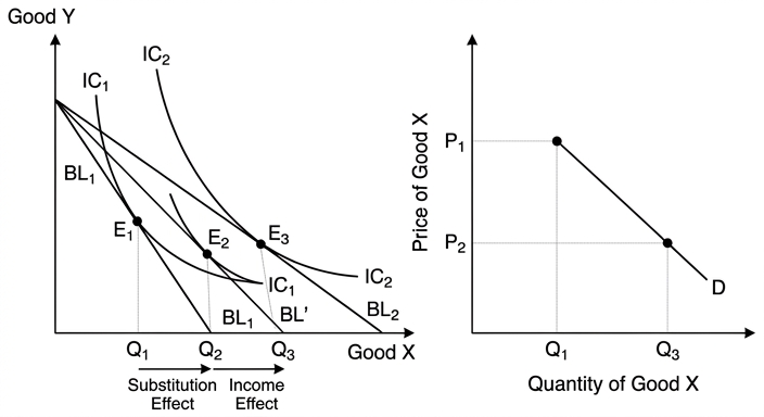
In the diagram, the consumer initially faces budget line BL1 and is at equilibrium E1, consuming Q1 of good X. A fall in the price of X pivots the budget line outward to BL2 (the intercept on the Y-axis unchanged, the X-intercept increases). The new equilibrium is at E3, consuming Q3 of X. The total increase in quantity demanded from Q1 to Q3 is the price effect.
This price effect can be decomposed into a substitution effect and an income effect. To isolate the substitution effect, a hypothetical budget line (BL') is drawn parallel to BL2 but tangent to the original indifference curve IC1. This shows the change in consumption due solely to the change in relative prices, holding real income constant. The substitution effect is the movement from E1 to E2 (Q1 to Q2). The income effect is the movement from E2 to E3 (Q2 to Q3), caused by the increase in real income from the price fall. For a normal good, both effects work in the same direction, so demand is downward-sloping.
By repeating this analysis for different prices, we can trace out the individual's demand curve for good X, showing the inverse relationship between price and quantity demanded.
Evaluation
Indifference curve analysis provides a rigorous theoretical foundation for the law of demand, separating the two effects that a price change has on consumer behaviour. However, its usefulness is limited by its assumptions:
- Rationality and completeness: The model assumes consumers can rank all bundles consistently and maximise utility. In reality, consumers may be influenced by habits, advertising, or bounded rationality, making indifference curves less stable.
- Two-good simplification: The analysis only considers two goods. In reality, consumers choose among many goods, and cross-price effects complicate the picture.
- Perfect information: Consumers are assumed to know their preferences and all prices. In practice, information is costly and imperfect.
- No change in tastes: The shape of indifference curves is assumed fixed. Advertising, fashions, or learning can shift preferences, altering the impact of a price change.
Despite these limitations, indifference curve analysis remains a powerful pedagogical tool. It clearly demonstrates that the demand curve is not merely a statistical relationship but is derived from utility-maximising behaviour. The decomposition into substitution and income effects is particularly valuable for understanding the response to price changes for different types of goods (normal, inferior, Giffen).
Conclusion
Indifference curve analysis is highly effective in explaining the relationship between a price change and individual demand, provided its assumptions are recognised. It offers a logically coherent framework that separates the substitution and income effects, which is essential for understanding demand. However, its predictive power in real markets is limited by behavioural complexities. Therefore, while it is a useful theoretical model, it should be applied with caution and supplemented by empirical evidence.
Indifference curve analysis effectively explains the price-demand relationship by decomposing the price effect into substitution and income effects, but its usefulness is constrained by assumptions of rationality, two-good simplification, and stable preferences; it remains a valuable theoretical framework when applied with awareness of its limitations.
Background Concept
Indifference curve analysis is a microeconomic model that represents consumer preferences graphically. An indifference curve (IC) shows all combinations of two goods that yield the same level of utility (satisfaction). The consumer is indifferent between any two points on the same IC. A family of ICs (indifference map) represents different utility levels; higher ICs correspond to higher satisfaction. The slope of an IC is the marginal rate of substitution (MRS), which diminishes as we move down the curve (diminishing marginal utility).
A budget line shows all combinations of two goods that a consumer can afford given their income and the prices of the goods. Its slope equals the negative of the price ratio (Px/Py). A change in the price of one good rotates the budget line around the intercept of the other good.
Consumer equilibrium occurs where the budget line is tangent to the highest attainable indifference curve. At this point, MRS = Px/Py, meaning the consumer's subjective valuation equals the market trade-off.
When the price of a good changes, the consumer moves to a new equilibrium. The total change in quantity demanded is the price effect, which can be decomposed into:
- Substitution effect: The change in consumption due to the change in relative prices, holding real income constant (movement along the original indifference curve).
- Income effect: The change in consumption due to the change in real income (purchasing power) caused by the price change, moving to a new indifference curve.
For normal goods, both effects work in the same direction (price fall increases quantity). For inferior goods, the income effect works opposite to the substitution effect. For Giffen goods, the income effect is so strong that it outweighs the substitution effect, leading to an upward-sloping demand curve.
Understanding the Question
The question asks you to "evaluate the use of indifference curve analysis to explain the relationship between a change in the price of a product and the change in an individual consumer's demand for this product." This is a 20-mark essay (AO1/AO2 out of 14, AO3 out of 6). The command word "evaluate" requires you to present both strengths and limitations of the analysis and reach a justified conclusion. The phrase "with the help of a diagram" means you must include a diagram; without one, the maximum mark is Level 2 (8 marks).
You need to:
- Explain indifference curves, budget lines, and consumer equilibrium.
- Show how a price change shifts the budget line and leads to a new equilibrium.
- Decompose the price effect into substitution and income effects (this is essential for Level 3).
- Derive the individual demand curve from the price-consumption path.
- Evaluate the assumptions of the model (rationality, two-good simplification, stable preferences, perfect information) and discuss its usefulness despite these limitations.
- Provide a justified conclusion.
Approach
- Introduction: Define indifference curve analysis and state its purpose.
- Analysis (AO1/AO2):
- Explain indifference curves, budget lines, and equilibrium.
- Describe the diagram: initial budget line, price fall, new budget line, new equilibrium.
- Decompose the price effect: substitution effect (hypothetical budget line) and income effect.
- Explain how this leads to the demand curve.
- Evaluation (AO3):
- Discuss strengths: rigorous theoretical foundation, separates effects, explains different types of goods.
- Discuss limitations: assumptions of rationality, two-good simplification, stable preferences, perfect information.
- Consider real-world applicability and the role of behavioural economics.
- Conclusion: Weigh the strengths against the limitations and give a justified judgement.
Step-by-Step Reasoning
Step 1: Set up the diagram
- Draw two axes: Good X on the horizontal, Good Y on the vertical.
- Draw an initial budget line (BL1) with intercepts determined by income and prices.
- Draw an indifference curve (IC1) tangent to BL1 at point E1. This is the initial equilibrium.
- Label the quantity of X at E1 as Q1.
Step 2: Show the price change
- Suppose the price of X falls. The budget line rotates outward: the Y-intercept stays the same (since Py and income unchanged), but the X-intercept increases. Draw the new budget line BL2.
- The consumer can now reach a higher indifference curve IC2. The new equilibrium is at E3, where BL2 is tangent to IC2. Label the quantity of X at E3 as Q3.
- The movement from Q1 to Q3 is the total price effect.
Step 3: Decompose the price effect
- To isolate the substitution effect, draw a hypothetical budget line (BL') that is parallel to BL2 (same price ratio) but tangent to the original indifference curve IC1. This line represents the budget needed to achieve the original utility at the new prices.
- The tangency point is E2. The movement from E1 to E2 (Q1 to Q2) is the substitution effect: the consumer substitutes towards the now relatively cheaper good X, holding real income constant.
- The movement from E2 to E3 (Q2 to Q3) is the income effect: the consumer's real income has increased (they can afford more of both goods), so they move to a higher indifference curve.
- For a normal good, both effects are positive (Q2 > Q1 and Q3 > Q2). For an inferior good, the income effect is negative (Q3 < Q2), but the substitution effect still positive, so the net effect depends on magnitudes. For a Giffen good, the negative income effect outweighs the substitution effect, so quantity demanded falls when price falls.
Step 4: Derive the demand curve
- By varying the price of X and recording the equilibrium quantities, we can plot the individual's demand curve for X. The price-consumption path (the line connecting E1, E3, etc.) shows how consumption of X changes with price. The demand curve is downward-sloping for normal goods.
Step 5: Evaluate
- Strengths: Provides a clear, logical explanation of the law of demand; separates substitution and income effects, which is crucial for understanding consumer behaviour; can explain exceptions like Giffen goods; forms the basis for welfare analysis (compensating variation, equivalent variation).
- Limitations:
- Rationality assumption: Consumers may not always maximise utility; they may be influenced by habits, emotions, or cognitive biases (behavioural economics).
- Two-good simplification: Real choices involve many goods; cross-price effects and budget constraints are more complex.
- Stable preferences: Tastes can change due to advertising, social influences, or learning, making indifference curves shift.
- Perfect information: Consumers may not know all prices or their own preferences perfectly.
- Indivisibility: Goods are often consumed in discrete units, not continuous bundles.
- Conclusion: Despite these limitations, indifference curve analysis remains a fundamental tool in microeconomics. It is highly effective for teaching the logic of demand and for understanding the components of a price change. However, its predictive power in real markets is limited; it should be complemented by empirical studies and behavioural insights. Overall, it is a useful but not perfect model.
Key Takeaways
- Indifference curve analysis provides a rigorous derivation of the demand curve from utility maximisation.
- The price effect is decomposed into substitution and income effects, which is essential for understanding consumer response to price changes.
- The model's assumptions (rationality, two-good world, stable preferences) are its main limitations.
- Evaluation should acknowledge both the theoretical strength and the practical weaknesses, leading to a balanced conclusion.
- A diagram is mandatory; without it, the maximum mark is capped at Level 2.
Common Mistakes
- Omitting the diagram: This caps the mark at Level 2 (max 8 marks). Always include a fully labelled diagram.
- Not decomposing the price effect: The mark scheme explicitly requires consideration of both substitution and income effects for Level 3. Simply showing two equilibria is insufficient.
- Confusing substitution and income effects: Ensure the hypothetical budget line is correctly drawn (parallel to new budget line, tangent to original indifference curve).
- One-sided evaluation: The question asks to "evaluate", so you must discuss both strengths and limitations. A one-sided answer cannot score high for AO3.
- Vague conclusion: The conclusion must be justified and address the specific question. Avoid simply saying "it depends".
- Not explaining the diagram: The diagram must be fully explained in the text; a diagram alone does not earn marks.
- Using incorrect labels: Axes, curves, and points must be clearly labelled (e.g., IC1, IC2, BL1, BL2, E1, E2, E3, Q1, Q2, Q3).
Things to Be Careful About
- Ensure the diagram is accurate: the hypothetical budget line must be parallel to the new budget line (same slope) and tangent to the original indifference curve.
- Distinguish between normal, inferior, and Giffen goods in the explanation of income effects.
- Use correct terminology: "substitution effect", "income effect", "price effect", "consumer equilibrium", "marginal rate of substitution".
- The evaluation should be developed, not just a list of criticisms. Explain why each limitation matters and how it affects the usefulness of the model.
- The conclusion should weigh the strengths against the weaknesses and give a clear judgement. For example: "Indifference curve analysis is a powerful theoretical tool for understanding the price-demand relationship, but its assumptions limit its direct applicability to real-world markets. Nevertheless, it remains essential for teaching and for welfare analysis."
The growth of a firm using a takeover is desirable because it enables consumers to benefit from lower prices and the firm to gain additional profits.
Evaluate this statement.
Introduction
A takeover occurs when one firm acquires control of another, often through purchasing a majority of its shares. This is a form of external growth. The statement claims that takeovers are desirable because they lead to lower prices for consumers and higher profits for the firm. This essay will evaluate both claims, considering the conditions under which they may or may not hold.
The case for lower prices and increased profits
A horizontal takeover (between firms in the same industry) can generate economies of scale. As the combined firm produces a larger output, average costs fall due to technical economies (specialisation, indivisibilities), managerial economies (spreading fixed management costs), purchasing economies (bulk discounts), financial economies (lower borrowing costs), and marketing economies (shared advertising). These cost reductions can be passed on to consumers as lower prices, benefiting them. At the same time, the firm’s profit margins may be maintained or even increased if the cost savings exceed the price reduction. Additionally, vertical integration (backward or forward) can reduce transaction costs and secure supply chains, further lowering costs and potentially increasing profits. For example, a car manufacturer taking over a parts supplier can reduce input costs and improve coordination, leading to lower final prices and higher profits.
The counter-arguments
However, the benefits are not guaranteed. First, the firm may use its increased market power to raise prices rather than lower them. A takeover that significantly increases market concentration can create monopoly power, allowing the firm to restrict output and charge higher prices, harming consumers. Second, diseconomies of scale may arise: the larger organisation may suffer from coordination problems, communication breakdowns, and culture clashes, increasing average costs and reducing profits. Third, the cost of the takeover itself (the premium paid to acquire the target, integration costs) can be substantial and may erode profits in the short and long run. Fourth, competition authorities may intervene to prevent anti-competitive outcomes, imposing price regulation or requiring divestitures, which can limit the firm’s ability to profit. Finally, the firm’s objective may not be profit maximisation; managers might pursue sales maximisation or other goals, leading to different outcomes.
Evaluation
The desirability of a takeover depends on several factors. In a contestable market with low barriers to entry, the threat of new entrants forces the merged firm to pass on cost savings as lower prices, benefiting consumers. In a concentrated market with high barriers, monopoly power is more likely to be exploited. The time period matters: short-run cost savings may be offset by long-run diseconomies. The type of integration also matters: horizontal takeovers are more likely to raise competition concerns, while vertical takeovers may be efficiency-enhancing. The firm’s post-merger strategy (whether it focuses on cost reduction or market power) is crucial.
Conclusion
The statement that takeovers are desirable because they lower prices and increase profits is not universally true. While takeovers can generate economies of scale and cost savings that benefit consumers and boost profits, they can also lead to monopoly power, diseconomies of scale, and reduced profits. The net effect depends on market structure, the type of integration, and the firm’s behaviour. Therefore, the desirability of a takeover is conditional, and the statement is an oversimplification.
Takeovers are not necessarily desirable; their impact on consumer prices and firm profits depends on market structure, the presence of economies or diseconomies of scale, and the firm's post-merger strategy, making the statement an oversimplification.
Background Concept
A takeover (or acquisition) is a form of external growth where one firm buys another. It differs from a merger, where two firms agree to unite as equals. Takeovers can be horizontal (same industry), vertical (different stages of production), or conglomerate (unrelated industries). The main economic rationale for takeovers is to achieve economies of scale, which reduce average costs as output increases. Economies of scale arise from specialisation, indivisibilities, bulk buying, cheaper finance, and spreading fixed costs. However, beyond a certain size, diseconomies of scale may set in due to coordination problems, bureaucracy, and loss of focus. Takeovers also affect market concentration, potentially increasing monopoly power, which allows the firm to raise prices and reduce output. The net effect on consumer welfare and firm profits depends on which force dominates.
Understanding the Question
The question asks you to evaluate the statement: "The growth of a firm using a takeover is desirable because it enables consumers to benefit from lower prices and the firm to gain additional profits." This is a normative statement claiming that takeovers are good for both consumers (lower prices) and the firm (higher profits). You must assess whether this is always, sometimes, or never true. The command word "Evaluate" requires you to present both sides of the argument and reach a justified conclusion. The marking scheme allocates 14 marks for AO1 (knowledge) and AO2 (analysis) combined, and 6 marks for AO3 (evaluation). The top band for AO1/AO2 requires detailed knowledge, fully developed explanations, and accurate use of concepts. The top band for AO3 requires a justified conclusion with developed evaluative comments.
Approach
- Define key terms: takeover, economies of scale, monopoly power, profits.
- Present the case for the statement: Explain how horizontal and vertical takeovers can lead to economies of scale, lower costs, lower prices, and higher profits. Use examples.
- Present the counter-arguments: Explain how takeovers can lead to monopoly power, higher prices, diseconomies of scale, and reduced profits. Also consider the role of competition authorities and managerial objectives.
- Evaluate: Weigh the conditions under which each outcome is more likely. Consider market structure, contestability, time period, type of integration, and firm strategy.
- Conclude: Provide a justified judgement that addresses the specific claim. The conclusion should not simply summarise but state whether the statement is valid and under what conditions.
Step-by-Step Reasoning
Step 1: Define takeover and distinguish from merger. A takeover is when one firm buys another, often against the target's will. This is external growth. The statement focuses on takeovers, not organic growth.
Step 2: Explain the case for lower prices and higher profits.
- Horizontal takeover: Two firms in the same industry combine. They can rationalise production, close duplicate plants, and specialise. This leads to economies of scale: average costs fall. For example, if two car manufacturers merge, they can share R&D, use the same parts, and negotiate better deals with suppliers. Lower costs can be passed on as lower prices, benefiting consumers. The firm may also increase its market share and total revenue, boosting profits. Even if prices fall, if costs fall more, profit per unit may rise.
- Vertical takeover: A firm takes over a supplier (backward) or a distributor (forward). This reduces transaction costs (search, negotiation, contract enforcement) and ensures quality and supply. For example, a coffee chain taking over coffee bean farms can secure supply and reduce costs, potentially lowering retail prices and increasing profits.
Step 3: Present the counter-arguments.
- Monopoly power: A takeover that significantly increases market share may give the firm market power. It can then restrict output and raise prices, harming consumers. The firm may choose to keep prices high rather than pass on cost savings. This is especially likely if barriers to entry are high.
- Diseconomies of scale: After a takeover, the larger firm may face coordination problems, communication breakdowns, and culture clashes. These increase average costs, reducing profits and potentially leading to higher prices if the firm tries to maintain margins.
- Cost of takeover: The acquiring firm often pays a premium to buy the target. This can be a large upfront cost that reduces profits. Integration costs (redundancies, rebranding, IT systems) also eat into profits.
- Competition authority intervention: Regulators may block the takeover or impose conditions (e.g., price caps, divestitures) that limit the firm's ability to raise prices or profits.
- Managerial objectives: Managers may pursue sales maximisation or growth for its own sake, not profit maximisation. They might overpay for a takeover, reducing profits.
Step 4: Evaluate the arguments.
- The net effect depends on the balance between economies of scale and market power. In a contestable market (low barriers to entry), the threat of new entrants forces the firm to pass on cost savings as lower prices. In a concentrated market with high barriers, monopoly power is more likely.
- The type of integration matters: horizontal takeovers are more likely to raise competition concerns than vertical ones. Vertical takeovers are often efficiency-enhancing and less likely to harm consumers.
- Time period: In the short run, cost savings may be realised, but in the long run, diseconomies may emerge. The takeover premium may be a one-time cost, but ongoing integration issues can persist.
- The firm's strategy: If the firm focuses on cost reduction and efficiency, consumers may benefit. If it focuses on market power, they may lose.
Step 5: Reach a justified conclusion.
The statement is an oversimplification. Takeovers can be desirable under certain conditions (e.g., contestable markets, vertical integration, effective management), but they can also be undesirable (e.g., horizontal takeovers in concentrated markets, poor integration). Therefore, the desirability is conditional, not universal.
Key Takeaways
- Takeovers can generate economies of scale, lowering costs and potentially prices.
- Takeovers can also increase monopoly power, leading to higher prices.
- Diseconomies of scale and integration costs can reduce profits.
- The outcome depends on market structure, type of integration, and firm behaviour.
- Evaluation requires considering both sides and reaching a conditional conclusion.
Common Mistakes
- One-sided answer: Only discussing benefits or only drawbacks. This loses all evaluation marks.
- No conclusion or a vague conclusion like "it depends" without specifying on what.
- Confusing takeover with merger (though similar, the distinction can be relevant).
- Ignoring the role of competition authorities.
- Failing to use economic terminology (economies of scale, monopoly power, contestability).
- Providing a list of points without developing the chain of reasoning.
Things to Be Careful About
- Ensure the conclusion is justified and addresses the specific statement (lower prices and additional profits).
- Use examples to support analysis (e.g., a specific industry).
- Distinguish between short-run and long-run effects.
- Consider both consumer and firm perspectives.
- The question is about takeovers, not all forms of growth. Stay focused.
A country is experiencing stagflation, when there is a high rate of inflation at the same time as a negative output gap.
With the help of a diagram, evaluate the effectiveness of using fiscal policy to solve this problem.
Introduction
Stagflation is the simultaneous occurrence of high inflation and a negative output gap, representing a dilemma for policymakers because the policy tools that address one typically worsen the other. Fiscal policy, which involves changes in government spending and taxation, can be used to influence aggregate demand (AD). However, its ability to solve stagflation is limited by the inherent conflict between the two objectives.
Analysis
A negative output gap exists when real GDP is below the potential level (Yfe), indicating unused resources and downward pressure on wages and prices. The situation can be illustrated with an AD/AS diagram.
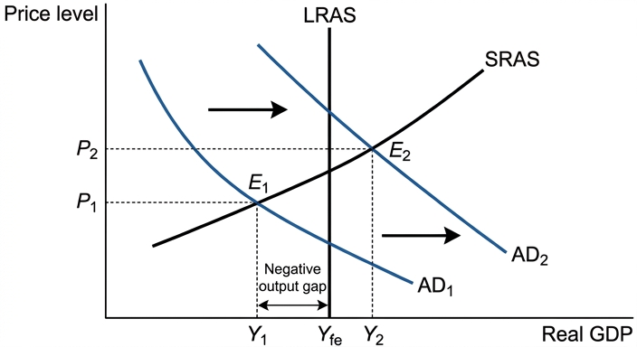
In the diagram, the economy is initially at equilibrium E1, with price level P1 and output Y1 below Yfe. The short-run aggregate supply (SRAS) curve is upward sloping and the long-run aggregate supply (LRAS) is vertical at Yfe. The negative output gap is the distance Yfe – Y1.
If the government uses expansionary fiscal policy – for example, increasing government spending or cutting taxes – AD shifts from AD1 to AD2. This raises output towards Yfe (Y2) and reduces the negative output gap. However, the price level rises to P2, worsening inflation. Conversely, contractionary fiscal policy (reducing spending or raising taxes) would reduce AD, lowering the price level and easing inflation, but would further increase the negative output gap. Thus, fiscal policy can only address one aspect of stagflation at a time.
Evaluation
The effectiveness of fiscal policy in solving stagflation is therefore limited because it cannot simultaneously close the output gap and reduce inflation. Expansionary fiscal policy risks accelerating inflation, especially if inflation expectations are already high. Contractionary fiscal policy could deepen unemployment and recession. Additionally, fiscal policy suffers from time lags (implementation and impact lags) that reduce its flexibility. Crowding out may also occur: expansionary fiscal policy financed by borrowing can raise interest rates, dampening private investment and offsetting some of the intended increase in AD.
Alternative policies, particularly supply-side measures, may be more effective. Supply-side policies (e.g., reducing regulation, investing in technology, improving labour market flexibility) aim to increase aggregate supply, shifting SRAS and LRAS to the right. This can simultaneously lower the price level and expand output, directly tackling both problems. However, supply-side policies often take time to implement and may cause short-run unemployment or require significant investment. In the short run, a combination of fiscal discipline to anchor inflation expectations and targeted supply-side reforms is often advocated.
Conclusion
In conclusion, fiscal policy alone is not highly effective in solving stagflation because it can only target one objective at the cost of the other. While it can be used to reduce the output gap (at the expense of higher inflation) or reduce inflation (at the expense of a larger output gap), it cannot resolve both simultaneously. Supply-side policies are more suited to addressing the root causes of stagflation, though they require time. Ultimately, the most effective strategy likely involves a mix of cautious fiscal policy to avoid destabilising demand and supply-side reforms to boost potential output and reduce cost pressures.
Fiscal policy is largely ineffective on its own in solving stagflation because expansionary measures worsen inflation while contractionary measures widen the output gap; supply-side policies offer a more comprehensive long-term solution.
Background Concept
Stagflation is a challenging macroeconomic situation combining high inflation with a negative output gap (actual output below potential output). The Phillips curve traditionally suggests a trade-off: low unemployment (high output) comes with higher inflation, and high unemployment (low output) with lower inflation. However, stagflation violates this simple trade-off, often caused by supply shocks (e.g., oil price hikes) that raise costs and reduce output simultaneously. The AD/AS model is used to analyse this: a negative supply shock shifts SRAS left, raising prices and reducing output. In this question, the root cause is not specified, but the problem presents a conflict for demand-side policies.
Understanding the Question
The question asks to evaluate the effectiveness of using fiscal policy to solve stagflation. This requires two-sided analysis: can fiscal policy simultaneously reduce inflation and close the negative output gap? The command word 'evaluate' demands a judgement on the extent to which fiscal policy is effective, weighing its strengths and weaknesses, and considering alternatives. The top band requires a justified conclusion. A diagram is mandatory and must be fully explained; marks are capped at 8 without one.
Approach
We begin by defining stagflation and the negative output gap. Then we draw an AD/AS diagram to show the initial situation and the effect of expansionary fiscal policy. We also discuss contractionary fiscal policy in prose. The analysis then moves to evaluation: the inherent conflict, time lags, crowding out, and the role of supply-side policies as an alternative. The conclusion should state the relative effectiveness of fiscal policy compared to supply-side measures, both in the short and long run.
Step-by-Step Reasoning
- Define stagflation: High inflation and negative output gap simultaneously. Explain that a negative output gap means actual GDP < potential GDP, implying spare capacity and unemployment. Inflation is high, typically due to cost-push factors or expectations.
- Draw the AD/AS diagram: Label axes (Price Level and Real GDP). Draw LRAS vertical at Yfe (potential output). Draw SRAS upward sloping. Draw AD1 sloping downward. Mark initial equilibrium E1 at intersection of AD1 and SRAS, with price level P1 and output Y1 (< Yfe). Shade the horizontal distance between Y1 and Yfe as the negative output gap.
- Show expansionary fiscal policy: Increase G or cut taxes -> AD shifts right from AD1 to AD2. New equilibrium E2 at intersection of AD2 and SRAS. Output rises to Y2 (closer to Yfe but possibly still below), price level rises to P2. This reduces the output gap but increases inflation.
- Discuss contractionary fiscal policy: Opposite effect: reduces inflation but widens output gap. Show that fiscal policy cannot address both simultaneously.
- Evaluate effectiveness: Limitations include: policy conflict, time lags (recognition, decision, implementation, impact), crowding out (government borrowing raises interest rates, reducing private investment), and possible ineffectiveness if the economy is in a liquidity trap or if expectations are anchored poorly. Also consider the role of automatic stabilisers but they are not sufficient.
- Alternative policies: Supply-side policies (e.g., deregulation, tax reforms to incentivise work and investment, infrastructure spending) can shift SRAS and LRAS to the right, reducing inflation and increasing output simultaneously. However, they take time and may cause short-term adjustment costs.
- Comparison and conclusion: In the short run, fiscal policy can target one objective but worsens the other. In the long run, supply-side policies are more effective at addressing the root causes. Therefore, the most effective approach combines cautious fiscal policy (to avoid destabilising the economy) with structural reforms. Fiscal policy alone is not highly effective.
Key Takeaways
- Stagflation presents a policy dilemma because demand-side policies face a trade-off between inflation and output.
- The AD/AS diagram is essential to visualise the conflict and the effects of fiscal policy.
- Evaluation should consider time lags, crowding out, and the superiority of supply-side policies in tackling both problems.
- A justified conclusion must weigh the relative effectiveness of different policies over different time horizons.
Common Mistakes
- Forgetting to include a diagram or drawing one without clear labels and explanation (capped at 8 marks).
- Only discussing one type of fiscal policy (e.g., only expansionary) without considering the alternative.
- Failing to address the simultaneous nature of the problem – many students treat inflation and output gap in isolation.
- Providing a one-sided evaluation without discussing supply-side policies or other alternatives.
- Ending with a summary rather than a justified conclusion that states the extent of effectiveness.
- Using vague terms like 'it depends' without specifying the conditions.
Things to Be Careful About
- Ensure all curves and equilibria are correctly labelled on the diagram (AD, SRAS, LRAS, Yfe, Y1, P1, P2, E1, E2).
- Clearly explain the chain of reasoning: how fiscal policy changes AD, and how that affects output and price level.
- Distinguish between short-run and long-run effects.
- Use the extract's implied context: the country is experiencing stagflation; it may be helpful to note that the cause (supply shock or demand) matters for policy effectiveness.
- Avoid over-claiming: fiscal policy is not entirely ineffective; it can partially address one objective, but not both at once.
- In the conclusion, judge the overall effectiveness relative to alternatives, not just list pros and cons.
A free trade area gains all the benefits associated with being a member of a customs union while avoiding all the costs associated with being a member of a customs union.
Evaluate this statement.
Introduction
A free trade area (FTA) is a bloc where member countries eliminate tariffs and quotas on trade among themselves but each retains its own trade policies towards non-members. A customs union (CU) goes further by adopting a common external tariff (CET) on imports from non-members. The statement claims that an FTA obtains all the benefits of a CU while incurring none of its costs. This essay evaluates that claim by comparing the benefits and costs of each arrangement.
Benefits shared by both an FTA and a CU
Both arrangements remove internal barriers to trade, which generates trade creation: the replacement of higher-cost domestic production with lower-cost imports from a partner country. This leads to a more efficient allocation of resources, greater specialisation according to comparative advantage, and economies of scale as firms access a larger market. Increased competition from partner firms can raise productivity and lower prices for consumers. These effects stimulate economic growth and raise living standards. Thus, an FTA does enjoy many of the core benefits of a CU.
Additional benefits of a customs union not available in an FTA
A CU's common external tariff provides a uniform level of protection against non-members, which can shield domestic industries from low-cost competition and allow them to grow. The larger, more integrated market of a CU may attract more foreign direct investment (FDI) because investors face a single set of trade rules for the whole bloc. A CU also tends to foster deeper political and economic cooperation, reducing the risk of conflict and facilitating further integration. These benefits are largely absent in an FTA, where each country sets its own tariffs, creating complexity for traders and potentially diverting investment to the most favourable entry point rather than the most efficient location.
Costs of a customs union that an FTA avoids
Membership of a CU involves a loss of sovereignty over trade policy: a country cannot independently negotiate trade deals or set its own tariffs. The CET may force a country to impose tariffs on imports from a non-member that it would prefer to admit freely, leading to trade diversion – switching from a more efficient non-member supplier to a less efficient partner-country supplier. This misallocates resources and reduces global welfare. Consumers may face higher prices on some goods because of the CET. An FTA avoids these costs because each member retains control over its external tariffs and can pursue its own trade agreements.
Costs specific to a free trade area
However, an FTA is not cost-free. The absence of a CET creates the problem of trade deflection: goods from non-members may enter the FTA through the country with the lowest external tariff and then move freely to other members. To prevent this, FTAs require complex rules of origin, which impose administrative and compliance costs on businesses. These costs can be significant, especially for small firms. Moreover, the lack of a unified external policy can lead to less coherent economic integration and may limit the scale of efficiency gains compared with a CU.
Evaluation
The statement that an FTA gains all the benefits of a CU is inaccurate because a CU offers additional advantages – particularly the protective and investment-attracting effects of a CET and deeper political integration – that an FTA does not provide. The claim that an FTA avoids all the costs of a CU is also overstated: while an FTA avoids the loss of sovereignty and trade diversion associated with a CET, it incurs its own costs from rules of origin and trade deflection. The net balance depends on the specific circumstances: for a country that values policy autonomy and trades mainly with partners that are already efficient, an FTA may be preferable; for a country seeking deep integration and protection from non-member competition, a CU may offer greater net benefits.
Conclusion
In conclusion, the statement is an overgeneralisation. A free trade area captures many but not all of the benefits of a customs union and avoids many but not all of its costs. The claim that it gains all benefits while avoiding all costs is therefore not supported by economic analysis.
The statement is an overgeneralisation: a free trade area gains many but not all benefits of a customs union (it lacks the common external tariff's protective benefits and deeper integration) and avoids many but not all costs (it faces its own costs such as rules of origin and trade deflection).
Background Concept
Economic integration refers to the process by which countries reduce barriers to trade and coordinate their economic policies. The two most basic forms are a free trade area (FTA) and a customs union (CU). In an FTA, member countries eliminate tariffs and quotas on trade among themselves but each maintains its own separate trade policies (including tariffs) towards non-members. In a CU, members also remove internal barriers but additionally adopt a common external tariff (CET) on imports from non-members. Deeper forms include common markets, economic unions, and full monetary unions.
The key economic concepts used to evaluate integration are trade creation and trade diversion. Trade creation occurs when a country switches from a higher-cost domestic producer to a lower-cost partner-country producer after internal barriers are removed, improving resource allocation and welfare. Trade diversion occurs when a country switches from a lower-cost non-member producer to a higher-cost partner-country producer because the CET makes the non-member's goods more expensive, worsening resource allocation. The net welfare effect of joining a CU depends on whether trade creation outweighs trade diversion.
Benefits of integration include: greater specialisation according to comparative advantage, economies of scale from access to larger markets, increased competition raising productivity and lowering prices, stimulus to foreign direct investment (FDI), and potential for deeper political cooperation. Costs include: loss of sovereignty over trade policy, trade diversion, administrative costs (e.g., rules of origin in FTAs), and possible unequal distribution of gains among members.
Understanding the Question
The question presents the statement: "A free trade area gains all the benefits associated with being a member of a customs union while avoiding all the costs associated with being a member of a customs union." The command word is "Evaluate", which requires a two-sided analysis and a justified conclusion. The statement contains two absolute claims: "all the benefits" and "all the costs". To evaluate it, we must compare the benefits and costs of an FTA and a CU, identify which benefits are shared, which are unique to a CU, which costs are unique to a CU, and whether an FTA has its own costs that the statement ignores. The conclusion must judge the extent to which the statement holds true.
Approach
- Define both terms clearly.
- Identify the benefits that both arrangements share (internal tariff removal, trade creation, specialisation, economies of scale, competition).
- Identify benefits that a CU offers but an FTA does not (common external tariff protection, greater FDI attraction, deeper political integration).
- Identify costs that a CU incurs but an FTA avoids (loss of sovereignty, trade diversion, potential higher consumer prices from CET).
- Identify costs that an FTA faces (rules of origin, trade deflection, less coherent integration).
- Weigh the evidence: does the FTA really gain "all" benefits? Does it really avoid "all" costs?
- Reach a justified conclusion that addresses the specific wording of the statement.
Step-by-Step Reasoning
Step 1: Define the terms. A free trade area eliminates internal tariffs and quotas but allows each member to set its own external tariffs. A customs union also eliminates internal barriers but adds a common external tariff. This difference is crucial because the CET is the source of both additional benefits and additional costs.
Step 2: Shared benefits. Both an FTA and a CU remove barriers to trade among members. This leads to trade creation: firms can import from the most efficient partner-country producer instead of producing at home at higher cost. Resources are reallocated to industries where the country has a comparative advantage. Firms can achieve economies of scale by serving the entire integrated market. Competition from partner firms forces domestic firms to become more efficient, lowering prices for consumers. These benefits are present in both arrangements, so an FTA does enjoy many of the core benefits of a CU.
Step 3: Additional benefits of a CU. The CET gives CU members a unified trade policy. This can protect domestic industries from low-cost competition outside the union, allowing them to grow and perhaps achieve economies of scale before facing global competition. The larger, more predictable market with a single set of trade rules can attract more FDI from non-member firms that want to access the whole union without navigating different tariff regimes. A CU often fosters deeper political cooperation and reduces the risk of trade wars among members. These benefits are not available in an FTA, where each country's separate tariffs create complexity and may discourage investment. Therefore, the claim that an FTA gains "all" benefits of a CU is false.
Step 4: Costs of a CU that an FTA avoids. Joining a CU means surrendering independent trade policy. A country cannot negotiate its own trade deals or set tariffs to suit its own interests. The CET may force it to impose tariffs on imports from a non-member that it would prefer to admit freely, leading to trade diversion: buying from a less efficient partner-country supplier instead of a more efficient non-member. This reduces global welfare and may raise consumer prices. An FTA avoids these costs because each member retains control over its external tariffs and can pursue its own trade agreements. So the statement that an FTA avoids "all" costs of a CU is partly true.
Step 5: Costs specific to an FTA. However, an FTA is not cost-free. Because members have different external tariffs, goods from non-members can enter through the country with the lowest tariff and then move freely to other members (trade deflection). To prevent this, FTAs require rules of origin that prove a good was substantially produced within the FTA. These rules impose administrative and compliance costs on businesses, which can be substantial, especially for small firms. The lack of a unified external policy can also lead to less coherent integration and may limit the scale of efficiency gains. Thus, the statement that an FTA avoids "all" costs is an overstatement because it ignores the costs inherent in the FTA structure.
Step 6: Evaluation. The statement makes two absolute claims. The first – that an FTA gains all benefits of a CU – is incorrect because a CU offers additional benefits (CET protection, FDI attraction, deeper integration) that an FTA does not. The second – that an FTA avoids all costs of a CU – is partially correct but incomplete: an FTA avoids the sovereignty loss and trade diversion of a CU, but it incurs its own costs (rules of origin, trade deflection). The net desirability of an FTA versus a CU depends on country-specific factors: a country that values policy flexibility and trades mainly with efficient partners may prefer an FTA; a country seeking deep integration and protection from non-member competition may prefer a CU.
Step 7: Conclusion. The statement is an overgeneralisation. An FTA does not gain all the benefits of a CU, nor does it avoid all costs (it has its own costs). Therefore, the claim is not supported by economic analysis.
Key Takeaways
- A free trade area and a customs union are distinct forms of economic integration, differing mainly in the treatment of external tariffs.
- Both generate trade creation, specialisation, economies of scale, and competition, but a customs union offers additional benefits (CET protection, FDI, deeper integration) at the cost of lost sovereignty and potential trade diversion.
- A free trade area avoids some costs of a customs union but introduces its own costs (rules of origin, trade deflection).
- Absolute statements ("all benefits", "all costs") are rarely accurate in economics; evaluation requires identifying what is gained and what is sacrificed.
- A strong evaluation weighs both sides and reaches a justified conclusion that addresses the specific wording of the question.
Common Mistakes
- One-sided answer: Only discussing benefits of an FTA or only costs of a CU, without considering the other side. This loses all evaluation marks.
- No conclusion: Ending with a summary rather than a judgement. The top band requires a justified conclusion.
- Ignoring trade diversion: Failing to mention that a CU can cause trade diversion, which is a key cost.
- Assuming an FTA has no costs: Overlooking rules of origin and trade deflection, leading to an incomplete evaluation.
- Confusing FTA and CU: Not clearly distinguishing the two, which undermines the analysis.
- Vague conclusion: Saying "it depends" without specifying on what or giving a clear verdict.
Things to Be Careful About
- Use precise definitions: an FTA removes internal barriers but each member sets its own external tariffs; a CU adds a common external tariff.
- Distinguish between static effects (trade creation/diversion) and dynamic effects (economies of scale, FDI, competition).
- When evaluating, consider both efficiency and sovereignty – these are different dimensions.
- Support arguments with examples (e.g., NAFTA as an FTA, the EU as a customs union) to strengthen the response.
- Ensure the conclusion directly addresses the statement: does the FTA gain "all" benefits and avoid "all" costs? The answer should be a clear "no" with reasoning.
- Avoid overcomplicating: focus on the key differences and the absolute nature of the claim.