Economics 9708/41 — May/June 2025
Cambridge A-Level · A Level Data Response and Essays · worked solutions for every part, with the mark scheme
Topics Effectiveness of Macroeconomic Policies · Employment and Unemployment · Economic Growth and Sustainability · Government Policies to Correct Market Failure · Indifference Curves and Budget Lines · Growth and Survival of Firms · +3 more
The influence of governments
People often talk as if governments can easily control economic outcomes.
Content removed due to copyright restrictions.
High-income countries decided to focus on economic growth realising that it was essential to generate revenues and taxes needed to pay for costly investments, for example, the storage of renewable energy, required to reduce the use of fossil fuels.
Sources: Irwin Stelzer, The Sunday Times, 29 January 2023
Ray Bourne, The Times, 9 February 2023
The article refers to structural unemployment. Explain what this means and whether it is the same as the natural rate of unemployment.
Answer
Structural unemployment occurs when there is a mismatch between the skills that workers possess and the skills demanded by available jobs, or a geographical mismatch between where workers live and where jobs are located. It is a long-term form of unemployment caused by changes in the structure of the economy, such as the decline of an industry or technological change.
The natural rate of unemployment is not the same as structural unemployment. The natural rate is the rate of unemployment that exists when the labour market is in equilibrium, and it includes both structural unemployment and frictional unemployment (the short-term unemployment that occurs as workers move between jobs). Therefore, structural unemployment is a component of the natural rate, but the two are not identical.
Structural unemployment is a mismatch of skills or location between workers and jobs. The natural rate of unemployment includes structural and frictional unemployment, so they are not the same.
Background Concept
Unemployment is a key macroeconomic objective. Economists classify unemployment by its cause to understand how to address it. The main types are:
- Frictional unemployment: short-term unemployment that occurs when workers are between jobs or entering the labour force for the first time. It is a natural part of a dynamic economy.
- Structural unemployment: a more persistent form caused by a fundamental mismatch between the skills or location of workers and the requirements of available jobs. This can arise from technological change, the decline of a major industry, or globalisation.
- Cyclical (demand-deficient) unemployment: caused by a lack of aggregate demand in the economy, typically during a recession.
- Seasonal unemployment: due to seasonal variations in demand for labour.
The natural rate of unemployment (also called the non-accelerating inflation rate of unemployment, or NAIRU) is the rate of unemployment that prevails when the labour market is in equilibrium and there is no cyclical unemployment. It consists of frictional and structural unemployment. It is the lowest rate of unemployment that can be sustained without causing inflation to rise.
Understanding the Question
The question asks for two things: first, to explain what structural unemployment means; second, to state whether it is the same as the natural rate of unemployment and explain why or why not. This is a straightforward definition and distinction question worth 3 marks. The mark scheme awards 2 marks for a correct definition of structural unemployment and 1 mark for correctly stating that they are not the same and giving a brief reason.
Approach
- Define structural unemployment precisely, mentioning the skill or geographical mismatch.
- Define the natural rate of unemployment briefly.
- State clearly that they are not the same, and explain that structural unemployment is a component of the natural rate, which also includes frictional unemployment.
Step-by-Step Reasoning
- Step 1: Define structural unemployment. The key idea is a mismatch. The worker's skills are not what employers need, or the jobs are in a different location. This is not a temporary problem; it requires retraining or relocation to solve. Examples include coal miners in a region where mines have closed, or factory workers whose jobs have been automated.
- Step 2: Define the natural rate of unemployment. This is the equilibrium rate. It is not zero because even in a healthy economy, some workers are frictionally unemployed (searching for the best job) and some are structurally unemployed (needing to retrain). The natural rate is the sum of frictional and structural unemployment.
- Step 3: Distinguish. Since the natural rate includes frictional unemployment as well as structural unemployment, they are not the same. Structural unemployment is a part of the natural rate, but the natural rate is a broader concept.
Key Takeaways
- Structural unemployment is a long-term mismatch; frictional is short-term search.
- The natural rate = frictional + structural unemployment.
- Understanding the type of unemployment is crucial for choosing the right policy (supply-side policies for structural, demand-side for cyclical).
Common Mistakes
- Confusing structural unemployment with cyclical unemployment. Structural is about the structure of the economy; cyclical is about the business cycle.
- Stating that the natural rate is zero or that it is the same as full employment. The natural rate is the rate at which there is no cyclical unemployment, but there is still frictional and structural unemployment.
- Failing to mention frictional unemployment when explaining why the natural rate is different from structural unemployment.
Things to Be Careful About
- Be precise: "mismatch of skills or location" is the core of the definition.
- The mark scheme explicitly awards 1 mark for stating they are not the same. Do not just define both; make the comparison.
- Keep the answer concise for a 3-mark question.
To keep unemployment low, one government used fiscal policy. Analyse how this policy can affect unemployment rates.
Answer
Fiscal policy involves the use of government spending and taxation to influence the level of aggregate demand (AD) and economic activity.
To reduce unemployment, a government can use expansionary fiscal policy. This involves increasing government spending (G) and/or decreasing direct taxes (e.g. income tax).
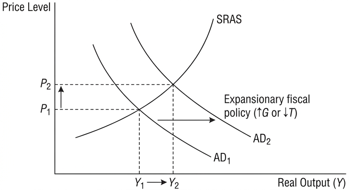
An increase in government spending directly increases AD (AD1 to AD2). Lower income taxes increase disposable income for households, leading to higher consumption (C), which further increases AD. The rise in AD shifts the AD curve to the right. At the initial price level, there is now excess demand. Firms respond by increasing output (Y1 to Y2) and therefore demand more labour to produce this higher output. This reduces demand-deficient (cyclical) unemployment.
The size of the effect on output and employment depends on the size of the multiplier. If the economy has spare capacity (a negative output gap), the increase in AD will lead to a larger increase in real output and a smaller increase in the price level. However, if the economy is already near full capacity, the policy may be more inflationary and less effective at reducing unemployment.
Furthermore, the effectiveness depends on the magnitude of the fiscal stimulus, the time lags involved in implementing the policy, and whether the increased government spending crowds out private sector investment.
Expansionary fiscal policy can reduce demand-deficient unemployment by increasing aggregate demand, which raises output and the demand for labour, provided the economy has spare capacity.
Background Concept
Fiscal policy is the use of government spending and taxation to influence the economy. It is a demand-side policy. The main components of aggregate demand (AD) are: AD = C + I + G + (X-M).
- Expansionary fiscal policy aims to increase AD. Tools include increasing government spending (G) or cutting taxes (which boosts consumption, C, and possibly investment, I).
- Contractionary fiscal policy aims to decrease AD. Tools include cutting government spending or raising taxes.
Unemployment can be caused by a lack of AD (cyclical/demand-deficient unemployment). If the economy is operating below full capacity, there is a negative output gap, and firms are not producing as much as they could. This means they employ fewer workers than they could. Increasing AD can close this gap and reduce unemployment.
The AD/AS model is the standard tool for analysing the impact of fiscal policy on output, employment, and the price level.
Understanding the Question
The question asks to "analyse how this policy can affect unemployment rates." The command word "analyse" requires a developed chain of reasoning. The mark scheme allocates 2 marks for defining fiscal policy, up to 4 marks for a correct diagram explained, and up to 2 marks for commenting on each example. This is a point-based question. The answer must show the mechanism clearly.
Approach
- Define fiscal policy (government spending and taxation).
- State that to reduce unemployment, the government would use expansionary fiscal policy.
- Explain the mechanism: an increase in G or a cut in taxes increases AD.
- Use an AD/AS diagram to illustrate the shift in AD and the resulting increase in real output (Y) and employment.
- Explain the chain of reasoning: higher AD -> higher output -> higher demand for labour -> lower unemployment.
- Add a brief evaluative comment on the conditions for effectiveness (spare capacity, multiplier, time lags, crowding out).
Step-by-Step Reasoning
- Step 1: Define the policy. Fiscal policy is the use of government spending and taxation. This is a necessary starting point for the analysis.
- Step 2: Identify the type of policy. To reduce unemployment, the government would use expansionary fiscal policy.
- Step 3: Explain the mechanism. An increase in government spending (G) directly adds to AD. A cut in income tax leaves households with more disposable income, which they spend on consumption (C), further increasing AD. A cut in corporation tax may encourage investment (I).
- Step 4: Use the diagram. The AD/AS diagram shows the initial equilibrium at price level P1 and real output Y1. Expansionary fiscal policy shifts the AD curve to the right (AD1 to AD2). The new equilibrium is at a higher price level (P2) and a higher level of real output (Y2).
- Step 5: Link to unemployment. To produce the higher level of output (Y2), firms need to employ more workers. This reduces demand-deficient unemployment. The chain of reasoning is: ↑G/↓T -> ↑AD -> ↑Y -> ↑demand for labour -> ↓unemployment.
- Step 6: Evaluate. The effectiveness depends on:
- Spare capacity: If the economy is in a recession with a large negative output gap, the increase in AD will mainly increase output and employment, with little inflation. If the economy is near full capacity, the increase in AD will be more inflationary and less effective at reducing unemployment.
- The multiplier: The final increase in Y is larger than the initial increase in G or C due to the multiplier effect.
- Time lags: There are recognition, decision, and implementation lags. By the time the policy takes effect, the economy may have recovered on its own.
- Crowding out: Increased government spending may be financed by borrowing, which pushes up interest rates and reduces private sector investment (I), offsetting some of the initial increase in AD.
Key Takeaways
- Fiscal policy is a demand-side tool.
- Expansionary fiscal policy can reduce cyclical unemployment by increasing AD.
- The AD/AS model is the key analytical tool.
- Effectiveness is conditional on spare capacity, the multiplier, time lags, and crowding out.
Common Mistakes
- Forgetting to define fiscal policy (costs 2 marks).
- Drawing a diagram but not explaining it. The explanation is where the marks are earned.
- Confusing a movement along the AD curve with a shift of the AD curve. Fiscal policy shifts AD.
- Only discussing the benefits without any evaluation. For a 6-mark "analyse" question, a brief evaluative comment is expected to show depth.
- Discussing supply-side effects. The question specifically asks about fiscal policy, which is a demand-side policy.
Things to Be Careful About
- Label the axes of the AD/AS diagram correctly: Price Level on the vertical axis, Real Output (Y) on the horizontal axis.
- Show the direction of the shift clearly (AD1 to AD2).
- Explain the chain of reasoning step-by-step.
- Keep the evaluation brief but relevant.
Explain how the policies of high-income economies towards ‘green energy’ changed between 2015 and 2022.
Answer
Between 2015 and 2022, the policies of high-income economies towards 'green energy' changed from a focus on reducing fossil fuel use and increasing green energy outputs, as agreed at the Paris Agreement, to a greater emphasis on economic growth. This shift was partly driven by the need to generate tax revenues to pay for costly investments, such as the storage of renewable energy. The article also suggests that promised funds from rich to poor countries for green energy did not materialise, and that poor countries were less effective in reducing CO2 emissions.
The policy shifted from a focus on reducing fossil fuels and increasing green energy (post-Paris Agreement) to a greater emphasis on economic growth by 2022, partly to generate tax revenues for green investments.
Background Concept
This question tests the ability to extract and interpret information from a given text (the article). It is a data-response skill. The article describes a change in the priorities of high-income countries regarding environmental policy.
Understanding the Question
The question asks to "explain how the policies of high-income economies towards 'green energy' changed between 2015 and 2022." The command word "explain" requires more than just stating the change; it requires describing the nature of the change and the reasons for it, as given in the text. This is a 3-mark question, so the answer should be concise but cover the key points from the mark scheme.
Approach
- Identify the policy stance in 2015 (around the Paris Agreement).
- Identify the policy stance in 2022.
- Explain the reason for the change as given in the text (need for economic growth to generate tax revenues).
- Mention any other relevant points from the text (e.g., unfulfilled promises to poor countries).
Step-by-Step Reasoning
- Step 1: Policy in 2015. The article refers to the Paris Agreement. At this time, high-income countries were willing to increase green energy outputs and reduce the use of fossil fuels in energy production.
- Step 2: Policy in 2022. By 2022, the focus had shifted. High-income countries decided to focus on economic growth. The article states this was because growth was "essential to generate revenues and taxes needed to pay for costly investments, for example, the storage of renewable energy, required to reduce the use of fossil fuels." This implies a temporary continuation of fossil fuel use to fund the transition.
- Step 3: Additional context. The article also mentions that promised funds from rich to poor countries did not materialise, and that poor countries were less effective in reducing CO2 emissions. This provides further context for the change in policy.
Key Takeaways
- Data-response questions require careful reading of the source material.
- The answer must be grounded in the text, not in general knowledge.
- Look for specific changes and the reasons given for them.
Common Mistakes
- Answering from general knowledge about climate change policy rather than from the article.
- Simply stating the change without explaining the reason for it.
- Providing too much detail for a 3-mark question.
Things to Be Careful About
- The question asks for the change "between 2015 and 2022." Make sure to describe the policy at both points in time.
- Use the specific language from the article where possible (e.g., "generate revenues and taxes").
Assess whether the article provides sufficient evidence to justify its conclusion that the intervention of governments has little effect on economic outcomes.
Answer
The article's conclusion is that government intervention has little effect on economic outcomes. However, the evidence provided in the article is mixed and does not fully justify this conclusion.
Evidence against the conclusion (governments DO have an effect):
- The war in Ukraine disrupted energy supplies, but this was a direct action by the Russian government. This shows government actions can have significant economic effects.
- Central banks raised interest rates to combat inflation. This is a direct government (or central bank) policy that affects economic outcomes like inflation and aggregate demand.
- The article states that governments decided to concentrate on growth rather than green energy. This decision itself is a government intervention that influenced the direction of the economy.
Evidence that supports the conclusion (governments have little effect):
- The article mentions that billions of private transactions occur, suggesting that private sector activity, not government policy, is the main driver of economic outcomes.
- The article does not provide evidence that supply-side policies were the reason for low unemployment in Germany, implying that other factors may have been more important.
- The link between fiscal policy and unemployment is presented as weak or unclear.
Evaluation: The article provides some evidence that governments can affect outcomes (e.g., interest rate rises, the war in Ukraine), but it also highlights the limitations of government power, especially in the face of large private sector forces and global events. The evidence is insufficient to justify the strong conclusion that governments have "little effect." A more balanced conclusion would be that governments can have a significant effect, but their power is constrained by external shocks, private sector behaviour, and the inherent complexities of the economy.
Conclusion: The article does not provide sufficient evidence to justify its conclusion. While it points to some limitations of government intervention, it also provides clear examples of government actions having major economic consequences, making the conclusion an overstatement.
No, the article does not provide sufficient evidence. It presents examples of government actions having significant effects (e.g., interest rate rises, the war in Ukraine) alongside examples of limitations, making the conclusion that governments have 'little effect' an overstatement.
Background Concept
This question is about evaluating the strength of evidence in an argument. It requires critical thinking skills. The article makes a claim (government intervention has little effect). The task is to assess whether the evidence presented in the article supports that claim. This involves identifying evidence that supports the claim, evidence that contradicts it, and then weighing the two to reach a judgement.
Government failure is a relevant concept. It refers to situations where government intervention leads to a net welfare loss, either because the intervention was ineffective or because it created new problems. The article's conclusion implies a form of government failure or impotence.
Understanding the Question
The question asks to "assess whether the article provides sufficient evidence to justify its conclusion." The command word "assess" requires a two-sided evaluation and a justified conclusion. This is an 8-mark point-based question. The mark scheme lists several pieces of evidence from the article and allocates up to 2 marks for explaining each point. It also explicitly reserves 1 mark for a conclusion. The answer must be structured to show both sides of the argument and end with a clear, justified verdict.
Approach
- State the article's conclusion clearly.
- Present the evidence from the article that SUPPORTS the conclusion (governments have little effect).
- Present the evidence from the article that CONTRADICTS the conclusion (governments DO have an effect).
- Evaluate the strength of the evidence on both sides. Which is more compelling? Is the evidence sufficient to justify the strong claim?
- Reach a justified conclusion that directly answers the question.
Step-by-Step Reasoning
- Step 1: Identify the conclusion. The article concludes that "the intervention of governments has little effect on economic outcomes." This is a strong, absolute claim.
- Step 2: Evidence SUPPORTING the conclusion.
- The article mentions "billions of private transactions." This suggests the private sector is the dominant force, dwarfing government action.
- The article does not give evidence that supply-side policies were the reason for low unemployment in Germany. This implies that the government's claimed success might be due to other factors.
- The link between fiscal policy and unemployment is presented as weak or unclear, suggesting that this tool of government is not very effective.
- Step 3: Evidence AGAINST the conclusion (showing government DOES have an effect).
- The war in Ukraine disrupted supplies. The article notes that the Russian government was responsible for the war and stopped the flow of natural gas. This is a clear example of a government action having a massive economic impact.
- Central banks raised interest rates to stop the rise in inflation. This is a direct policy action (monetary policy, often conducted by an independent central bank acting on behalf of the government) that affects borrowing, spending, and inflation.
- The article states that governments decided to concentrate on growth and did not direct finances to encourage 'green energy'. This decision itself is a government intervention that affected the economic outcome (the pace of the green transition).
- Step 4: Evaluation. The evidence against the conclusion is strong. The examples of the war in Ukraine and interest rate rises are clear, direct examples of government actions having major consequences. The evidence supporting the conclusion is weaker. The fact that private transactions are large does not mean government actions have "little effect"; governments set the rules of the game (regulation, property rights, etc.) that make those transactions possible. The lack of evidence for one policy (supply-side in Germany) does not prove that all government policies are ineffective. Therefore, the evidence is insufficient to justify the strong conclusion.
- Step 5: Conclusion. The article does not provide sufficient evidence. The conclusion is an overstatement. A more accurate conclusion would be that governments can have significant effects, but their power is not absolute and is constrained by various factors.
Key Takeaways
- "Assess" requires a two-sided argument and a justified conclusion.
- In data-response questions, the evidence must come from the text.
- A strong conclusion directly answers the question and is based on the preceding evaluation.
- Be critical of the evidence: is it sufficient to support the claim?
Common Mistakes
- Writing a one-sided answer (only supporting or only contradicting the conclusion). This would lose marks for evaluation.
- Failing to reach a conclusion. The mark scheme reserves a mark for this.
- Reaching a conclusion that is a summary of both sides ("there is evidence for and against") without a judgement. The conclusion must state which side is stronger and why.
- Using general knowledge about government failure instead of the specific evidence from the article.
- Not explaining how each piece of evidence relates to the conclusion.
Things to Be Careful About
- The question asks about the SUFFICIENCY of the evidence in the article. The answer must focus on what the article does and does not say.
- The conclusion must be justified by the analysis that precedes it.
- For an 8-mark question, aim for a well-structured answer with clear paragraphs for each side and a separate conclusion.
With the help of a diagram, evaluate the use of indifference curve analysis to explain the relationship between a change in the price of a product and the change in an individual consumer’s demand for this product.
Introduction
Indifference curve analysis is a tool used to model consumer choice between two goods. It shows how a rational consumer maximises utility given their budget constraint. A change in the price of a product alters the budget line and leads to a new equilibrium, which can be decomposed into a substitution effect and an income effect. This essay will use indifference curve analysis to explain the change in demand following a price change and evaluate the usefulness and limitations of this approach.
Analysis: The Price Effect and the Diagram
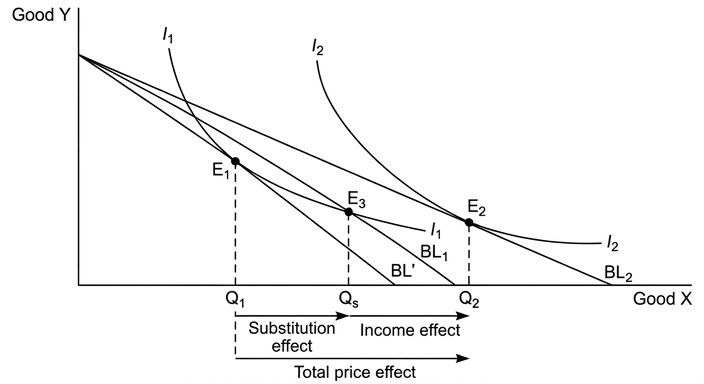
The diagram shows a consumer with a given money income choosing between Good X and Good Y. Initially, the budget line is BL1, and the consumer maximises satisfaction at point E1, where the budget line is tangent to indifference curve I1. The quantity of X demanded is Q1.
Now suppose the price of Good X falls. The budget line pivots outwards to BL2, as the consumer can now afford more of X with the same income. The new equilibrium is at E2 on a higher indifference curve I2, demanding Q2 of X. The total change in quantity demanded from Q1 to Q2 is the price effect.
The price effect can be decomposed into two parts:
- Substitution effect: The change in relative prices, holding real income constant. This is shown by drawing a hypothetical budget line (BL') parallel to BL2 but tangent to the original indifference curve I1. The substitution effect moves the consumer from E1 to E3, increasing quantity demanded from Q1 to Qs. This effect is always negative for a price fall (more of the cheaper good).
- Income effect: The change in purchasing power, shown by the movement from E3 to E2, as the consumer moves to a higher indifference curve. For a normal good, the income effect reinforces the substitution effect, leading to an overall increase in demand from Q1 to Q2. For an inferior good, the income effect works in the opposite direction, reducing the total increase, and for a Giffen good, the income effect outweighs the substitution effect, resulting in a downward-sloping demand curve.
Thus, indifference curve analysis provides a clear visual and theoretical explanation of how a price change affects individual demand, distinguishing between the two underlying effects.
Evaluation
However, the usefulness of indifference curve analysis is limited by its assumptions.
First, it assumes that consumers are rational and can consistently rank their preferences. In reality, consumers may be influenced by advertising, habits, or cognitive biases, making their preferences less stable than the model assumes.
Second, the model only considers two goods. Consumers typically choose from many goods, and the substitution effect may be spread across multiple goods, making the simple two-good diagram an oversimplification.
Third, the model assumes that the consumer is a price taker with perfect information. In practice, consumers may not have full information about prices or their own preferences, and they may face transaction costs.
Fourth, the indifference curve analysis does not account for changes in tastes or preferences. If a price change is accompanied by advertising, the indifference curve map itself may shift, altering the final outcome.
Despite these limitations, the model is a powerful tool for understanding the theoretical underpinnings of demand. It provides a rigorous framework for separating substitution and income effects, which is not possible with simple demand curves. It also helps explain exceptions such as Giffen goods.
Conclusion
Indifference curve analysis is highly effective in explaining the relationship between a price change and individual demand, as it identifies the separate roles of substitution and income effects. However, its predictive power is limited by its unrealistic assumptions. In simple, well-defined theoretical contexts, it is an excellent teaching tool, but it may not always accurately predict real-world behaviour, especially when preferences are influenced by external factors. Therefore, while it is a useful starting point, it should be supplemented with other models of consumer behaviour.
Indifference curve analysis is useful for explaining the price-demand relationship by decomposing the price effect into substitution and income effects, but its assumptions of rationality and the two-good simplification limit its real-world applicability.
Background Concept
Indifference curve analysis is a microeconomic model of consumer choice. An indifference curve represents all combinations of two goods that give the consumer the same level of utility or satisfaction. The indifference curve is downward sloping and convex to the origin, reflecting the diminishing marginal rate of substitution (the amount of one good the consumer is willing to give up for an additional unit of the other good while maintaining the same utility). A budget line shows all combinations of the two goods that the consumer can afford given their income and the prices of the goods. The consumer maximises utility at the point where the budget line is tangent to the highest attainable indifference curve. This is the consumer equilibrium.
A change in the price of one good shifts the budget line: a price fall pivots the budget line outward (the intercept on the axis of the good whose price has fallen moves outward), while a price rise pivots it inward. The change in quantity demanded of the good following a price change is called the price effect. This can be decomposed into a substitution effect (the change in consumption due to the change in relative prices, holding real income constant) and an income effect (the change in consumption due to the change in purchasing power, holding relative prices constant). For a normal good, both effects work in the same direction; for an inferior good, they oppose each other; for a Giffen good, the income effect is so strong that it outweighs the substitution effect, leading to an upward-sloping demand curve.
Understanding the Question
The question asks you to evaluate the use of indifference curve analysis to explain the relationship between a change in the price of a product and the change in an individual consumer's demand for that product. The command word is "evaluate", which means you must provide a balanced assessment: you need to explain how the model works (the analysis) and then critically assess its strengths and weaknesses, arriving at a justified conclusion. The question explicitly requires a diagram, and the mark scheme states that without a diagram the maximum mark is Level 2 (8 out of 14 for AO1/AO2). The question is from Paper 4 (A Level) and is worth 20 marks, split as AO1/AO2 out of 14 and AO3 out of 6. To achieve the top band, you must demonstrate detailed knowledge, fully developed analysis, a clearly explained diagram, and well-supported evaluative comments leading to a justified conclusion.
Approach
- Start with a brief introduction defining indifference curve analysis and the consumer equilibrium concept.
- Draw and explain a diagram showing the price effect for a normal good (most common case). Show the initial budget line and indifference curve, then the new budget line after a price fall, and the new equilibrium. Decompose the total change into substitution and income effects using a hypothetical budget line.
- Explain the substitution and income effects in words, linking them to the diagram.
- Discuss the strengths of the model: it provides a rigorous theoretical foundation for demand, distinguishes between substitution and income effects, and explains Giffen goods.
- Then evaluate the limitations: unrealistic assumptions (rationality, perfect information, only two goods, stable preferences), the impact of advertising and habit, and the difficulty of empirical application.
- Conclude with a justified judgement on the overall usefulness of the model.
Step-by-Step Reasoning
Step 1: Setting up the diagram
Draw a diagram with Good X on the horizontal axis and Good Y on the vertical axis. Draw a downward-sloping budget line BL1, representing the initial prices and income. Draw an indifference curve I1 convex to the origin, tangent to BL1 at point E1. This is the initial equilibrium; the consumer buys Q1 of X.
Step 2: Price fall
Suppose the price of X falls. The budget line pivots outward to BL2: the intercept on the X-axis increases (more X can be bought with the same income), while the intercept on the Y-axis remains unchanged. The new budget line is steeper (since the price of X has fallen relative to Y). The consumer reaches a new equilibrium at E2, where BL2 is tangent to a higher indifference curve I2. The quantity of X demanded increases to Q2.
Step 3: Decomposition
To separate the substitution and income effects, draw a hypothetical budget line BL' that is parallel to BL2 (same relative prices) but tangent to the original indifference curve I1. This line represents the budget the consumer would need to achieve the original utility level at the new prices. The tangency point is E3. The movement from E1 to E3 is the substitution effect: the consumer substitutes towards the cheaper good (X) while maintaining the same utility, so quantity increases from Q1 to Qs. The movement from E3 to E2 is the income effect: the consumer moves to a higher indifference curve because the price fall has increased real income. For a normal good, quantity increases further from Qs to Q2.
Step 4: Linking to demand
The price effect is the sum of substitution and income effects. For a normal good, both effects work in the same direction, so demand increases. For an inferior good, the income effect is negative, so the total increase is smaller. For a Giffen good, the negative income effect is so large that it outweighs the substitution effect, leading to a decrease in quantity demanded when price falls (a positively sloped demand curve). Indifference curve analysis can capture this.
Step 5: Evaluation
- Strengths: The model provides a clear theoretical framework for understanding consumer behaviour. It is internally consistent and allows for the decomposition of price effects, which is not possible with simple demand curves. It can explain exceptions like Giffen goods, which are paradoxical in ordinary demand theory.
- Limitations: The model assumes the consumer is rational and has complete, transitive preferences. Behavioural economics shows that real consumers often exhibit cognitive biases and inconsistent preferences. The model only considers two goods, which is a simplification; in reality, choices involve many goods, and the substitution effect may be spread across them. The model assumes perfect information and no transaction costs, which is unrealistic. It also assumes that preferences are stable and independent of prices, but advertising and social influences can change preferences. The diagram is static and does not easily incorporate dynamic factors like learning or habit formation.
- Conclusion: Despite these limitations, indifference curve analysis remains a valuable pedagogical tool for understanding the theoretical foundations of demand. It is most useful in simplified, controlled settings. For predicting real-world behaviour, it should be supplemented with insights from behavioural economics and empirical data. Therefore, while it is not a perfect predictor, it is a useful starting point for analysis.
Key Takeaways
- Indifference curve analysis decomposes the price effect into substitution and income effects, providing a deeper understanding of consumer demand.
- The model is based on assumptions of rationality, stable preferences, and two-good world, which limit its real-world applicability.
- The diagram is essential for full marks; it must be accurately drawn and fully explained.
- Evaluation should be balanced and lead to a justified conclusion that addresses the specific question.
Common Mistakes
- Omitting the diagram: The mark scheme explicitly states that without a diagram the highest mark is L2 (8 marks). Always include a diagram when asked.
- Not explaining the diagram: Simply drawing the diagram is not enough; you must explain what each part shows, linking it to the theory.
- Failing to decompose the price effect: Many students only show the overall change from E1 to E2 without the substitution and income effects. The mark scheme requires both effects to be considered for Level 3.
- One-sided evaluation: The question asks to "evaluate", so you must discuss both strengths and limitations. One-sided answers lose AO3 marks.
- No conclusion: The top band requires a justified conclusion. A summary without a judgement is insufficient.
- Confusing substitution and income effects: Make sure you correctly identify which movement is which.
- Forgetting to label axes and curves: Labels are part of the diagram marks; ensure all curves, points, and axes are clearly labelled.
Things to Be Careful About
- Label the axes: Good X and Good Y.
- Label the budget lines: BL1, BL2, BL'.
- Label the indifference curves: I1, I2.
- Label the equilibrium points: E1, E2, E3.
- Indicate the quantities: Q1, Qs, Q2.
- Show the direction of the price change (pivot of budget line).
- Clearly distinguish between substitution and income effects in the diagram and in the text.
- Mention that the analysis assumes a normal good initially, but you can also discuss inferior and Giffen goods in the evaluation.
- In the evaluation, avoid vague statements; be specific about the assumptions and their implications.
- The conclusion should state whether the model is useful or not, and under what conditions.
- The essay should be well-organised and coherent, with clear paragraphs.
The growth of a firm using a takeover is desirable because it enables consumers to benefit from lower prices and the firm to gain additional profits.
Evaluate this statement.
Introduction
A takeover occurs when one firm acquires control of another, often classified as horizontal (same industry stage), vertical (different stages), or conglomerate. The statement claims that such growth is desirable because it leads to lower prices for consumers and additional profits for the firm. This essay evaluates the validity of this claim by examining the potential benefits and drawbacks of takeovers.
Benefits of takeovers
Horizontal takeovers can generate economies of scale, which reduce average costs. As the firm expands, it can benefit from technical economies (specialisation, larger machinery), managerial economies (spreading fixed management costs), financial economies (access to cheaper finance), and marketing economies (bulk advertising). Lower average costs enable the firm to reduce prices if competitive pressure exists, benefiting consumers. Additionally, the takeover increases the firm's market share, potentially raising total revenue and profits if the cost savings are not fully passed on. Vertical integration, whether backward (acquiring a supplier) or forward (acquiring a distributor), can also reduce costs by eliminating profit margins in the supply chain and improving coordination, again potentially lowering prices and increasing profits.
Drawbacks of takeovers
However, the desirability is not guaranteed. A takeover may increase the firm's market power, allowing it to act as a monopolist. With greater monopoly power, the firm can restrict output and raise prices above the competitive level, harming consumers. The cost savings from economies of scale may be retained as higher profits rather than passed on as lower prices, especially if demand is inelastic. Furthermore, takeovers can lead to diseconomies of scale. Integrating two different corporate cultures, management styles, and information systems can create coordination problems, reduce efficiency, and increase average costs. The cost of the takeover itself—paying a premium to acquire the target, legal and advisory fees, and restructuring expenses—can also reduce profits in the short and long run. Additionally, competition authorities may intervene to prevent excessive concentration, imposing price regulation or blocking the takeover, which limits the firm's ability to raise prices or achieve expected synergies.
Evaluation
Whether the statement holds depends on several factors. In a competitive market with low barriers to entry, any cost savings are likely to be passed on to consumers as firms compete for market share, and profits may be normal rather than supernormal. In a concentrated market, the acquiring firm may exploit its market power to raise prices, making the takeover undesirable for consumers. The net effect on profits depends on whether the efficiency gains from economies of scale outweigh the costs of integration and any diseconomies. In the short run, profits may increase due to cost savings and increased market share, but in the long run, diseconomies and regulatory intervention may erode them. The type of integration matters: horizontal integration is more likely to generate economies of scale but also raises competition concerns, while vertical integration may improve efficiency without significantly increasing market power. The desirability also depends on the perspective: from the firm's viewpoint, additional profits are desirable, but from society's viewpoint, lower prices and consumer welfare are more important.
Conclusion
In conclusion, the statement that takeover growth is desirable because it enables lower prices and additional profits is not universally true. It is most likely to hold when the takeover leads to substantial economies of scale that are passed on to consumers due to competitive pressures, and when the firm successfully avoids diseconomies of scale and regulatory constraints. However, where the takeover creates monopoly power, leads to diseconomies, or is excessively costly, the benefits may not materialise, and the takeover may be undesirable for consumers and even for the firm in the long run. Therefore, a balanced assessment is necessary, and the statement should be accepted only under specific conditions.
The statement is not universally true; takeovers can lead to lower prices and higher profits when they generate economies of scale in a competitive market, but they may harm consumers and reduce profits when they create monopoly power or diseconomies of scale.
Background Concept
Takeovers (or acquisitions) are a form of external growth where one firm buys another. They can be horizontal (same industry and stage), vertical (different stages of production), or conglomerate (unrelated businesses). The main economic rationale for takeovers is to achieve economies of scale—reductions in long-run average cost as output increases—which can arise from technical, managerial, financial, marketing, and risk-bearing economies. Economies of scale are typically illustrated by a downward-sloping long-run average cost (LRAC) curve. However, beyond a certain scale, diseconomies of scale may set in due to coordination and communication problems, causing LRAC to rise. Takeovers also affect market structure: they increase concentration and may grant the firm market power, enabling it to influence price. The trade-off between efficiency gains and market power is central to evaluating the desirability of takeovers.
Understanding the Question
The question presents a statement: "The growth of a firm using a takeover is desirable because it enables consumers to benefit from lower prices and the firm to gain additional profits." The command word is "Evaluate", which requires a two-sided analysis and a justified conclusion. The statement makes two specific claims: (1) consumers benefit from lower prices, and (2) the firm gains additional profits. The evaluation must consider both claims and assess whether they hold under various circumstances. The question is from Paper 4 (A Level) and carries 20 marks, with AO1+AO2 out of 14 and AO3 out of 6. The top band requires detailed knowledge, fully developed explanations, accurate use of concepts, and a justified conclusion with developed evaluative comments.
Approach
The essay should be structured as follows:
- Introduction: Define takeover and state the purpose of the evaluation.
- Analysis of the benefits: Explain how takeovers can lead to economies of scale, lower costs, and potentially lower prices and higher profits. Use the concepts of horizontal and vertical integration.
- Analysis of the drawbacks: Discuss how takeovers can lead to monopoly power, higher prices, diseconomies of scale, costly integration, and regulatory intervention.
- Evaluation: Weigh the conditions under which the benefits outweigh the drawbacks. Consider market structure, time period, type of integration, and regulatory environment.
- Conclusion: Provide a justified judgement that answers the specific question, stating whether the statement is generally true, partially true, or false, and under what conditions.
Step-by-Step Reasoning
Benefits chain:
- A horizontal takeover combines two firms in the same industry, increasing the scale of operations.
- Larger scale allows specialisation of labour and capital, leading to technical economies: average fixed costs fall as output rises, and more efficient machinery can be used.
- Managerial economies: fixed management costs (e.g., CEO salary, head office) are spread over more output.
- Financial economies: larger firms often obtain lower interest rates on loans and better terms from suppliers.
- These economies reduce the long-run average cost (LRAC) of production.
- In a competitive market, firms are price takers; to sell the increased output, the firm must lower price to match competitors. Thus, cost savings are passed on to consumers as lower prices.
- Even if the firm has some market power, it may choose to lower price to increase sales and maximise profit if demand is elastic.
- The takeover also increases the firm's market share, which can increase total revenue. If average cost falls, profit per unit rises, leading to additional total profits.
- Vertical integration (backward or forward) can reduce costs by eliminating the profit margins of suppliers or distributors, improving coordination, and ensuring quality and supply reliability. These savings can also be passed on as lower prices.
Drawbacks chain:
- A takeover increases market concentration. If the combined firm gains significant market share, it may acquire monopoly power, allowing it to set price above marginal cost.
- With monopoly power, the firm can restrict output and raise price to maximise profit, harming consumers. The cost savings from economies of scale may be retained as higher profit rather than passed on.
- The extent of price increase depends on the price elasticity of demand: if demand is inelastic, the firm can raise price significantly without losing many sales.
- Diseconomies of scale: integrating two firms can be complex. Different corporate cultures, management styles, and IT systems can lead to coordination failures, reduced morale, and inefficiencies. These increase average costs, offsetting any economies of scale.
- The takeover itself is costly: the acquiring firm often pays a premium over the target's market value, plus legal, advisory, and restructuring costs. These costs reduce profits and may take years to recoup.
- Competition authorities (e.g., CMA in the UK) may investigate mergers that substantially lessen competition. They may impose remedies such as price caps, require divestitures, or block the takeover entirely, limiting the firm's ability to raise prices or achieve expected synergies.
Evaluation:
- The net effect on prices and profits depends on the balance between efficiency gains and market power. If economies of scale are substantial and the market remains competitive (e.g., low barriers to entry, many rivals), prices are likely to fall and profits may be normal. If the takeover creates a dominant firm with high barriers to entry, prices may rise and profits may be supernormal in the short run but attract entry or regulation.
- The time horizon matters: in the short run, integration costs and diseconomies may reduce profits, but in the long run, if synergies are realised, profits may increase. However, long-run diseconomies may eventually erode profits.
- The type of integration: horizontal integration is more likely to generate economies of scale but also raises competition concerns. Vertical integration may improve efficiency without significantly increasing market power, making it more likely to benefit consumers.
- From the firm's perspective, additional profits are desirable, but from society's perspective, lower prices and consumer welfare are more important. The statement's desirability is ambiguous.
- A justified conclusion: The statement is not universally true. It holds when the takeover leads to genuine efficiency gains that are passed on to consumers due to competitive pressures, and when the firm avoids diseconomies and regulatory hurdles. It fails when the takeover creates monopoly power, leads to diseconomies, or is excessively costly. Therefore, the desirability of a takeover must be assessed on a case-by-case basis.
Key Takeaways
- Takeovers can generate economies of scale, reducing costs and potentially lowering prices and increasing profits.
- However, they can also lead to monopoly power, diseconomies of scale, and costly integration, which may harm consumers and reduce profits.
- Evaluation requires considering market structure, elasticity of demand, time period, type of integration, and regulatory environment.
- A justified conclusion must address the specific claims of the statement and weigh the conditions.
Common Mistakes
- Writing a one-sided answer that only discusses benefits or only drawbacks; this loses all evaluation marks.
- Failing to provide a conclusion or providing a vague conclusion that does not address the specific statement.
- Listing points without developing chains of reasoning; e.g., stating "economies of scale lead to lower prices" without explaining how.
- Using incorrect or imprecise terminology (e.g., confusing takeover with merger, or economies of scale with economies of scope).
- Ignoring the "additional profits" part of the statement and focusing only on consumer prices.
- Not using real-world examples or context to support arguments (though not required, examples strengthen analysis).
- Including irrelevant material, such as discussing organic growth or other forms of integration not related to takeovers.
Things to Be Careful About
- Clearly distinguish between a takeover and a merger; the question specifically says "takeover".
- Ensure that the analysis of lower prices is linked to the mechanism of economies of scale and competitive pressure.
- When discussing monopoly power, explain how it allows the firm to raise prices, not just assert it.
- Consider both short-run and long-run effects; diseconomies of scale often appear in the long run.
- In the conclusion, explicitly state whether the statement is valid, and under what conditions.
- Use economic terminology accurately: economies of scale, diseconomies of scale, monopoly power, market concentration, barriers to entry, price elasticity of demand.
- Avoid making unsupported claims; each point should be logically developed.
A country is experiencing stagflation, when there is a high rate of inflation at the same time as a negative output gap.
With the help of a diagram, evaluate the effectiveness of using fiscal policy to solve this problem.
Introduction
Stagflation combines high inflation and a negative output gap (actual output below potential). This poses a dilemma for fiscal policy because policies that close the output gap (expansionary) tend to worsen inflation, while policies that reduce inflation (contractionary) widen the output gap.
Analysis of the Problem
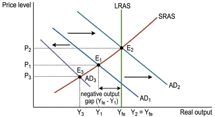
The diagram shows the initial position at E1: output Y1 is below full employment Yfe, indicating a negative output gap, yet the price level P1 is high, reflecting cost‑push or expectational factors. This is the stagflation scenario.
The Case for Using Fiscal Policy to Close the Output Gap
Expansionary fiscal policy (e.g., increased government spending or tax cuts) shifts AD rightwards to AD2. This raises output towards Yfe, reducing unemployment and closing the negative output gap. However, the price level rises to P2, worsening inflation. In the short run, the multiplier effect amplifies the demand stimulus, but if the economy is supply‑constrained (SRAS steep), most of the impact falls on prices rather than output.
The Case Against: Fiscal Policy to Reduce Inflation
Contractionary fiscal policy (e.g., spending cuts or tax increases) shifts AD leftwards to AD3. This reduces the price level to P3, curbing inflation. But output falls further to Y3, widening the negative output gap and raising unemployment. This is the classic policy conflict: the Phillips curve trade‑off (in the short run) implies that reducing inflation comes at the cost of even lower output and higher unemployment.
Evaluation
Fiscal policy alone cannot solve both problems simultaneously. The underlying cause of stagflation is often a supply‑side shock (e.g., rising oil prices) that shifts SRAS leftwards, raising costs and prices while reducing output. In such a case, demand‑management policies treat the symptom, not the cause.
- Time horizon: Expansionary fiscal may temporarily close the gap but at the cost of higher inflation, which may become entrenched if expectations adjust. Contractionary fiscal may reduce inflation but at the cost of deeper recession.
- Effectiveness depends on SRAS elasticity: If SRAS is nearly vertical (full capacity), fiscal policy mainly affects prices; if more elastic, it affects output more.
- Crowding out: Expansionary fiscal may crowd out private investment, reducing its long‑run effectiveness.
- Alternative policies: Supply‑side policies (e.g., deregulation, productivity improvements, training) can shift SRAS and LRAS rightwards, simultaneously reducing inflation and closing the output gap in the long run. However, they often take time and may have short‑run adjustment costs.
- Policy mix: A combined approach – e.g., moderate expansionary fiscal to support output coupled with structural reforms to boost supply – may be more effective than relying solely on fiscal policy.
Conclusion
Fiscal policy is of limited effectiveness in solving stagflation because it addresses only the demand side of the economy. Expansionary fiscal risks entrenching inflation; contractionary fiscal deepens the output gap. The most effective solution requires supply‑side measures to raise potential output and reduce costs, possibly supplemented by cautious demand management to avoid excessive recession. In the short run, supply‑side policies are slower, so a temporary tolerance of inflation while closing the gap may be necessary if inflation expectations are not strongly anchored.
Fiscal policy alone is ineffective in solving stagflation because it cannot simultaneously correct a negative output gap and reduce inflation; the optimal response requires supply‑side policies to address the root cause, with fiscal policy used cautiously to limit recessionary damage.
Background Concept
Stagflation is a macroeconomic situation where an economy experiences both high inflation and a negative output gap (actual output below potential output, i.e., above‑normal unemployment). This is unusual because, according to the traditional Phillips curve, inflation and unemployment are inversely related in the short run: high inflation should accompany low unemployment (positive output gap), not high unemployment. Stagflation typically arises from a negative supply‑side shock – e.g., a sharp rise in oil prices or other input costs – that shifts the short‑run aggregate supply (SRAS) curve leftwards, raising the price level and reducing output at the same time. Fiscal policy refers to changes in government spending and taxation to influence aggregate demand (AD). Because stagflation has both demand‑side and supply‑side dimensions, a single demand‑management tool like fiscal policy faces a trade‑off: it can target either the output gap or inflation, but not both simultaneously.
Understanding the Question
The question asks you to evaluate the effectiveness of using fiscal policy to solve stagflation. You are explicitly told that the country has high inflation and a negative output gap. The command word “evaluate” requires you to present both sides of the argument – the potential benefits and the drawbacks – and then reach a justified conclusion. The instruction “with the help of a diagram” means you must include a clearly labelled aggregate demand and aggregate supply (AD/AS) diagram and explain it in the text. The top band (Table A) expects “detailed knowledge and understanding”, “fully developed” explanations, and “accurate and relevant use of analytical tools such as diagrams”. Table B expects a “justified conclusion or judgement” with “developed, reasoned and well‑supported evaluative comments”. The question does not specify a split between AO1/AO2 and AO3, but the mark scheme allocates 14 marks to AO1/AO2 and 6 to AO3. So your answer must demonstrate strong theoretical knowledge (definition of stagflation, negative output gap, fiscal policy) and analysis (how fiscal policy shifts AD, the Phillips curve trade‑off) for the first 14 marks, and then provide a well‑reasoned evaluation weighing alternatives, time horizons, and underlying causes for the additional 6 marks.
Approach
- Set the scene: Define stagflation and the negative output gap. Explain why it is a problem. Introduce fiscal policy.
- Use the diagram: Draw an AD/AS diagram showing the initial stagflation equilibrium – output below full employment (negative gap) but a high price level. Label all curves and points.
- First side – expansionary fiscal: Explain how an increase in G or a cut in T shifts AD right, closing the output gap. But acknowledge that this worsens inflation. Use the diagram to illustrate (shift from AD1 to AD2).
- Second side – contractionary fiscal: Explain how a decrease in G or rise in T shifts AD left, reducing inflation. But this widens the output gap and raises unemployment. Use the diagram (shift from AD1 to AD3).
- Evaluation: Discuss why fiscal policy alone is insufficient. Mention the supply‑side nature of stagflation – the root cause is often a leftward SRAS shift. Discuss time lags, crowding out, the shape of SRAS, and the role of expectations. Contrast with supply‑side policies that can shift both SRAS and LRAS right, addressing both problems. Evaluate the relative effectiveness: fiscal works on demand but cannot fix supply; supply‑side works on both but takes time and may have adjustment costs. Conclude that a policy mix is likely best, but fiscal policy is of limited effectiveness alone.
- Conclusion: Give a justified judgement – e.g., fiscal policy can help manage one dimension but cannot solve stagflation; supply‑side reforms are essential; a combination may be optimal but requires careful calibration.
Step-by-Step Reasoning
- Step 1: Define the problem. Stagflation = high inflation + negative output gap. A negative output gap means actual GDP is below potential GDP, suggesting spare capacity and unemployment. But inflation is high, which is inconsistent with a simple demand‑pull explanation. This points to a supply‑side shock (cost‑push inflation).
- Step 2: Draw the AD/AS diagram. Label price level (P) on the vertical axis, real output (Y) on the horizontal. Draw downward‑sloping AD1, upward‑sloping SRAS, and vertical LRAS at Yfe. The initial equilibrium (E1) is where AD1 and SRAS intersect, at Y1 < Yfe and P1 (high). Show the negative output gap as the horizontal distance between Y1 and Yfe.
- Step 3: Expansionary fiscal. Suppose government increases spending or cuts taxes. This raises aggregate demand, shifting AD to AD2. The new equilibrium (E2) is at the intersection of AD2 and SRAS, at Y2 = Yfe (gap closed) but P2 > P1 (more inflation). This shows the output gap can be closed, but inflation worsens. Discuss the multiplier – the initial stimulus leads to further rounds of spending, but the eventual effect depends on how close the economy is to full capacity. If SRAS is steep (supply constraints), most of the stimulus goes into prices.
- Step 4: Contractionary fiscal. Suppose government reduces spending or raises taxes. This reduces AD, shifting AD to AD3. New equilibrium (E3) at Y3 < Y1 (wider gap) and P3 < P1 (less inflation). This shows inflation can be reduced, but at the cost of even lower output and higher unemployment.
- Step 5: Evaluation. The crux is that stagflation is not a standard demand‑deficit problem; it involves a supply constraint. Fiscal policy works only on demand, so it can treat one symptom only by aggravating the other. The effectiveness also depends on:
- The slope of SRAS: If SRAS is relatively flat (elastic), expansionary fiscal boosts output a lot with little extra inflation; if steep, it mostly raises prices.
- Time lags: Fiscal policy takes time to implement and have effect (inside and outside lags). By the time it works, the economy may have adjusted, making the policy less timely.
- Crowding out: Increased government spending might raise interest rates, reducing private investment, which weakens the expansionary effect in the long run.
- Expectations: If people expect higher inflation, they may demand higher wages, shifting SRAS left even further, making the trade‑off worse. Contractionary fiscal may help anchor expectations but at a high output cost.
- Supply‑side alternatives: Policies that improve productivity, reduce regulation, invest in infrastructure, or encourage innovation can shift SRAS and LRAS right, thus reducing the price level and increasing output simultaneously – a win‑win. However, these take time to yield results and may involve short‑run adjustment costs (e.g., unemployment from automation).
- Step 6: Conclusion. Fiscal policy alone is not very effective for stagflation because it cannot address the supply‑side root cause. A combination of moderate expansionary fiscal to support employment while implementing supply‑side reforms to boost potential output is more promising. In the short run, some inflation may be tolerated to avoid deeper recession, but the ultimate solution lies in raising productivity and reducing costs. Therefore, the effectiveness of fiscal policy is limited unless complemented by supply‑side measures.
Key Takeaways
- Stagflation is a dilemma: demand‑side policies cannot solve both inflation and output gap simultaneously.
- The AD/AS diagram is essential to illustrate the trade‑off and the initial position.
- Evaluation should consider time horizon, elasticity of SRAS, crowding out, expectations, and alternative policies (supply‑side).
- A justified conclusion must weigh these factors and give a clear verdict.
- Avoid a one‑sided answer – both expansionary and contractionary cases must be explained.
Common Mistakes
- One‑sided answer: Only discussing either expansionary or contractionary fiscal. The question asks to evaluate effectiveness, which requires both sides.
- No diagram or poorly labelled diagram: Without a diagram, maximum 8 marks. All curves must be labelled (AD, SRAS, LRAS, initial equilibrium, shifts, output gap).
- Confusing movement along with shift: Fiscal policy shifts AD, not SRAS. Some students mistakenly shift SRAS when explaining demand management.
- Ignoring the supply side: Treating stagflation as a normal recession and only recommending demand expansion. The high inflation component signals that supply factors matter.
- Vague conclusion: Ending with “it depends” without stating what it depends on and which side is stronger. The top band requires a justified judgement.
- Lack of development: Listing points without building causal chains (e.g., “expansionary fiscal increases demand, which increases output, which reduces unemployment” – need to explain the transmission mechanism including multiplier and price effects).
Things to Be Careful About
- In the diagram, clearly show the negative output gap (distance between Y1 and Yfe) and label it. Also ensure that the price level is shown to be high (relative to the full‑employment equilibrium that would occur if SRAS shifted appropriately).
- Use correct terminology: “negative output gap” not “recession” (though recession describes a period, output gap is specific).
- Distinguish between short run and long run. Fiscal policy works on AD; supply‑side policies affect AS. The evaluation must consider these time dimensions.
- When discussing “effectiveness”, specify the criterion: effective for what? Reducing inflation? Closing output gap? Both? The conclusion should state that fiscal policy is ineffective for solving both simultaneously, but can be effective for one if the other is sacrificed.
- Avoid over‑claiming. For example, do not say fiscal policy can never work – it can partially address one aspect, but not both. The evaluation should acknowledge conditional effectiveness.
- Remember to integrate the diagram explanation into the text: refer to the diagram when presenting the shifts and outcomes.
- Use data or examples where possible? The question does not provide extract, but you can refer to generic examples such as the 1970s oil price shocks.
- Keep the answer focused on the question: “fiscal policy to solve this problem”. Do not wander into monetary policy or exchange rate policy unless as part of evaluation comparison.
- Ensure the conclusion directly answers the question: “evaluate the effectiveness of using fiscal policy”. The final judgement should be clear: limited because of the inherent trade‑off, but can play a supporting role with supply‑side policies.
A free trade area gains all the benefits associated with being a member of a customs union while avoiding all the costs associated with being a member of a customs union.
Evaluate this statement.
Introduction
A free trade area (FTA) and a customs union (CU) are both forms of economic integration that remove internal tariffs and quotas among member countries. However, a CU additionally introduces a common external tariff (CET) against non-members. The statement claims that an FTA achieves all the benefits of a CU while avoiding all its costs. This essay evaluates the extent to which this is true by comparing the benefits and costs of each.
The Case for the Statement
An FTA does provide many of the same benefits as a CU. Both arrangements eliminate tariffs on trade between members, leading to trade creation: resources are reallocated from high-cost domestic production to lower-cost member production, increasing efficiency and welfare. Both also widen the market, allowing firms to exploit economies of scale. This can stimulate economic growth, raise incomes, and increase competition, which may improve labour productivity. Crucially, an FTA avoids several costs specific to a CU. A CU requires members to surrender control over their own trade policy by adopting a CET. This reduces national sovereignty and may force a country to impose tariffs on imports from non-members that it would prefer to keep low. An FTA, by contrast, allows each member to maintain its own external tariffs. This flexibility can be beneficial if a country's trade interests lie outside the bloc. Furthermore, the CET in a CU can cause trade diversion: a member may switch from a more efficient non-member producer to a less efficient member producer simply because the non-member's goods are now subject to the tariff. This misallocates resources and reduces global welfare. An FTA, with its independent external tariffs, is less likely to generate such trade diversion because members can still import freely from the cheapest global source and pay only their own national tariff. Thus, an FTA appears to capture the efficiency gains of internal free trade without the cost of a common trade policy or the risk of trade diversion.
The Case Against the Statement
Despite these points, an FTA does not achieve all the benefits of a CU. The CET in a CU creates a single, larger integrated market that is more attractive to foreign direct investment (FDI) from outside the bloc. Firms wishing to serve the whole CU market can locate production anywhere inside and export freely to all members, while facing a uniform tariff on imports from outside. This can lead to greater inward FDI, technology transfer, and deeper integration than an FTA, where differing external tariffs create complexity and reduce the incentive to invest. A CU also tends to foster closer political cooperation and stability, as members must coordinate trade policy. This can reduce transaction costs and uncertainty, further boosting trade and investment. Moreover, the benefits of trade creation in a CU may be larger than in an FTA because the CET eliminates the need for rules of origin. In an FTA, goods may be subject to complex rules of origin to prevent trade deflection (importing from outside via the low-tariff member and then re-exporting tariff-free). These rules impose administrative costs and can act as non-tariff barriers, reducing the gains from trade. A CU avoids this entirely. Finally, the claim that an FTA avoids trade diversion is not entirely accurate. An FTA can still cause trade diversion if a firm sources from a higher-cost member to avoid the tariff that would be paid on a cheaper non-member import, especially if the non-member's tariff is high. Thus, trade diversion is not exclusive to CUs.
Evaluation
The statement is an oversimplification. While an FTA avoids the specific cost of losing trade policy sovereignty and the associated risk of trade diversion from a CET, it does not provide the same depth of market integration, attractiveness to FDI, or political cohesion as a CU. The administrative burden of rules of origin in an FTA is a real cost that the CU avoids. Moreover, the benefits of trade creation may be more extensive in a CU because of the larger, unified market and the absence of internal barriers beyond tariffs. The magnitude of these differences depends on the specific blocs: for example, a deep FTA with harmonised rules can mimic some CU benefits, while a CU with high external tariffs may cause significant trade diversion. The net effect varies.
Conclusion
The statement is incorrect. A free trade area does not gain all the benefits of a customs union, as it lacks the deeper market integration, FDI attraction, and political stability that a customs union can offer. Nor does it avoid all costs, because it imposes rules of origin and still faces the possibility of trade diversion. The choice between an FTA and a CU involves a trade-off between sovereignty and deeper integration; the optimal arrangement depends on a country's specific economic and political circumstances.
The statement is not supported; a free trade area does not achieve all the benefits of a customs union and does not avoid all its costs, as the two forms of integration involve different trade-offs between sovereignty, market depth, and administrative complexity.
Background Concept
Free trade areas (FTAs) and customs unions (CUs) are two types of regional trade agreements that aim to increase trade among member countries. In an FTA, members eliminate tariffs and quotas on trade among themselves but each retains its own external tariff on imports from non-members. In a CU, members also eliminate internal barriers but additionally adopt a common external tariff (CET) on imports from non-members. Both arrangements can generate trade creation – the replacement of high-cost domestic production by lower-cost imports from a member – which improves allocative efficiency and raises welfare. However, they also risk trade diversion – the replacement of cheaper imports from a non-member by more expensive imports from a member because of the tariff advantage. CUs are generally considered a deeper form of integration because they require coordination of trade policy, and they may also lead to greater foreign direct investment (FDI) and political cohesion. FTAs typically require rules of origin to prevent trade deflection (goods entering the bloc through the member with the lowest external tariff). These rules impose administrative costs and can act as non-tariff barriers.
Understanding the Question
This question presents a statement: 'A free trade area gains all the benefits associated with being a member of a customs union while avoiding all the costs associated with being a member of a customs union.' The command word is 'Evaluate', which demands a two-sided analysis and a justified conclusion. The statement makes two specific claims: (1) an FTA achieves all the benefits of a CU, and (2) an FTA incurs none of the costs of a CU. Your task is to assess the truth of both claims. The mark scheme awards AO1/AO2 (14 marks) for knowledge and analysis, and AO3 (6 marks) for evaluation. The top band requires detailed knowledge, fully developed explanations, and a well-organised response. The evaluation must be developed, reasoned, and well-supported, leading to a justified conclusion that addresses the specific question.
Approach
The essay will be structured as follows:
- Introduction: Define FTA and CU, and state the claim to be evaluated.
- The case for the statement: Explain how an FTA does provide many benefits of a CU (e.g., trade creation, economies of scale, growth) and avoids some costs (e.g., loss of sovereignty, trade diversion from CET).
- The case against the statement: Explain how an FTA fails to achieve some benefits of a CU (e.g., deeper market integration, FDI attraction, political stability, no rules of origin) and also incurs some costs of its own (e.g., rules of origin, possible trade diversion).
- Evaluation: Weigh the two sides, using criteria such as the depth of integration, the magnitude of trade creation/diversion, and the administrative burden. Acknowledge that the outcome depends on the specific blocs.
- Conclusion: Provide a clear judgement on the statement.
Step-by-Step Reasoning
Step 1: Define the key terms.
- A free trade area (FTA) eliminates internal tariffs and quotas among members but allows each member to set its own trade policy with non-members.
- A customs union (CU) goes further by adopting a common external tariff (CET) on imports from non-members.
- The statement claims that an FTA gets all the benefits of a CU while avoiding all its costs.
Step 2: Analyse the benefits common to both.
- Both FTAs and CUs remove tariffs on intra-bloc trade, leading to trade creation. For example, if Country A removes a tariff on imports from Country B, consumers in A switch from a higher-cost domestic producer to a lower-cost B producer, increasing efficiency and consumer surplus. This is a benefit of both arrangements.
- Both widen the market, allowing firms to achieve economies of scale, which lowers average costs and can lead to lower prices for consumers. This can stimulate economic growth and raise incomes.
- Both increase competition among member firms, which can improve productivity and innovation.
Step 3: Identify the costs of a CU that an FTA allegedly avoids.
- Loss of trade policy sovereignty: In a CU, members must agree on a common external tariff; they cannot independently negotiate trade deals with non-members. An FTA preserves this sovereignty.
- Trade diversion caused by the CET: If the CET is higher than a member's previous tariff, the member may be forced to switch from a cheaper non-member producer to a dearer member producer, resulting in a net welfare loss. The FTA's independent tariffs reduce this risk.
- Political constraints: CU members may need to coordinate on other policies, reducing flexibility.
Step 4: Analyse the benefits of a CU that an FTA does not fully achieve.
- Deeper market integration: The CET creates a single market that is more attractive to FDI. For example, a non-member firm might set up a factory in a CU member to serve the entire bloc without facing multiple sets of tariffs. In an FTA, differing external tariffs create complexity, reducing the incentive to invest. This is a benefit of CU that an FTA cannot replicate.
- Political stability and cooperation: A CU often requires deeper political cooperation, which can reduce uncertainty and transaction costs, further boosting trade and investment. An FTA typically involves less political integration.
- No rules of origin: In an FTA, goods must meet rules of origin to qualify for tariff-free treatment, which adds administrative costs and can act as non-tariff barriers. A CU eliminates this entirely because the CET ensures that once goods enter the bloc, they can circulate freely without such checks. This is a cost of an FTA that the statement ignores.
- Larger trade creation effects: The absence of rules of origin in a CU means that trade creation can be more extensive within the bloc, as firms face no bureaucratic hurdles.
Step 5: Analyse the costs of an FTA that the statement overlooks.
- Rules of origin impose administrative costs and can be used as protectionist tools. For example, complex rules may make it expensive for firms to prove origin, reducing the benefits of tariff elimination.
- Trade diversion can still occur in an FTA: if a member's external tariff on a non-member good is high, a firm may source from a higher-cost member to avoid the tariff. This is trade diversion, and it is not exclusive to CUs.
- Lack of a common external tariff can lead to trade deflection, where goods from non-members enter the bloc through the member with the lowest tariff and then move tariff-free to other members. This can undermine the integrity of the FTA and require costly enforcement mechanisms.
Step 6: Evaluate the overall claim.
- The statement is an overgeneralisation. An FTA does achieve some benefits of a CU (trade creation, economies of scale) and avoids some costs (sovereignty loss, trade diversion from CET). However, it does not achieve all benefits: it lacks the deeper market integration, FDI attraction, and political stability of a CU. It also incurs costs that are not present in a CU, such as rules of origin and the possibility of trade deflection. Therefore, the claim that an FTA gains 'all the benefits' and avoids 'all the costs' is false.
- The extent of the difference depends on the specific blocs. For example, a very deep FTA with harmonised rules of origin and strong dispute resolution may approach the benefits of a CU. Conversely, a CU that sets a very high CET may cause significant trade diversion, making the FTA option more attractive. The evaluation must be nuanced.
Step 7: Formulate a justified conclusion.
- The conclusion should state that the statement is not supported. A free trade area does not achieve all the benefits of a customs union and does not avoid all its costs. The choice between them involves a trade-off between sovereignty and deeper integration. The judgement should be based on the analysis above and should be specific to the question.
Key Takeaways
- Understand the differences between an FTA and a CU: the key distinction is the presence of a common external tariff in a CU.
- Recognise that trade creation and trade diversion are central concepts for evaluating trade blocs.
- Learn to evaluate a 'strong' statement by breaking it into its component claims (all benefits, all costs) and testing each against economic theory.
- Develop the ability to construct a two-sided argument and reach a justified conclusion.
Common Mistakes
- One-sided argument: Only presenting the benefits of an FTA and ignoring the costs, or vice versa. The question requires an evaluation of both sides.
- Not addressing the specific claim: Failing to compare the FTA and CU directly, or discussing general benefits of trade blocs without reference to the statement.
- Lack of depth: Listing points without developing the chain of reasoning. For example, simply stating 'trade creation occurs' without explaining how and why.
- No conclusion or a vague conclusion: The top band requires a justified conclusion. A summary of both sides is not sufficient; the conclusion must make a judgement.
- Ignoring the cost side: The statement mentions 'avoiding all costs', so it is essential to identify costs that an FTA does not avoid (e.g., rules of origin) and costs that it does avoid (e.g., loss of sovereignty).
- Overgeneralisation: The answer should acknowledge that the differences depend on the specific blocs.
Things to Be Careful About
- Use precise definitions: Free trade area and customs union must be defined correctly.
- Distinguish between trade creation and trade diversion: They are opposite effects; trade creation improves welfare, trade diversion reduces it.
- Remember that trade diversion can occur in both FTAs and CUs, but the mechanisms differ.
- Mention rules of origin as a specific cost of FTAs; this is a key point that the statement overlooks.
- Consider dynamic effects: FDI, economies of scale, and political stability are important for evaluation.
- Ensure the conclusion directly answers the question: Is the statement correct? Yes/No and why.
- Avoid being too simplistic: The statement is an exaggeration, but the evaluation should show that there are trade-offs, not just a blanket rejection.
- Use appropriate economic terminology throughout (e.g., 'allocative efficiency', 'comparative advantage', 'trade creation', 'trade diversion', 'rules of origin', 'common external tariff').