Economics 9708/31 — May/June 2025
Cambridge A-Level · A Level Multiple Choice · answer key with instant marking and worked solutions
Topics Government Policies to Correct Market Failure · Macroeconomic Objectives and Policy Conflicts · Externalities, Social Costs and Benefits · Wage Determination and Labour Market Intervention · Employment and Unemployment · Money and Banking · +14 more
Tap an option under each question to check it — your score builds as you go.
What is the equi-marginal principle?
Options
A As consumption of a product increases, the satisfaction from consumption of the product decreases by an equal amount.
B Consumers maximise utility where their marginal valuation for each product consumed is the same.
C The total satisfaction received by consumers from consumption of a product is constant.
D The marginal utility derived by consumers from the consumption of one more unit of a product is constant.
Answer
The equi-marginal principle states that a consumer maximises total utility when the marginal utility per unit of currency spent is equal across all goods consumed. This is equivalent to option B: consumers maximise utility where their marginal valuation for each product consumed is the same.
B
Background Concept
The equi-marginal principle is a fundamental rule in consumer theory. It explains how a rational consumer with a limited income allocates their spending across different goods to achieve the highest possible total satisfaction (utility). The principle is derived from the law of diminishing marginal utility: as a person consumes more of a good, the additional (marginal) utility from each extra unit falls. To maximise utility, the consumer should not spend all their money on the good that gives the highest initial marginal utility, because as they consume more of it, its marginal utility falls. Instead, they should spread their spending so that the last unit of currency spent on each good yields the same marginal utility. In formal terms, the condition for consumer equilibrium is:
MUa / Pa = MUb / Pb = ... = MUn / Pn
where MU is marginal utility and P is price. This ratio is sometimes called the marginal utility per dollar (or per unit of currency).
Understanding the Question
This is a straightforward multiple-choice question that asks for the definition of the equi-marginal principle. The four options present different statements about utility. The task is to select the one that correctly and completely describes the principle. The question tests knowledge of a specific concept within utility theory, not its application or calculation.
Approach
Read each option carefully and compare it to the standard definition of the equi-marginal principle. Eliminate options that describe other concepts (like the law of diminishing marginal utility or constant marginal utility). The correct option will state that consumers maximise utility by equalising the marginal valuation (or marginal utility per unit of currency) across all goods.
Step-by-Step Reasoning
-
Option A: "As consumption of a product increases, the satisfaction from consumption of the product decreases by an equal amount." This describes the law of diminishing marginal utility, but it is imprecise (satisfaction doesn't decrease by an equal amount each time). More importantly, it is a statement about a single good, not about the allocation of spending across multiple goods. This is not the equi-marginal principle. Eliminate.
-
Option B: "Consumers maximise utility where their marginal valuation for each product consumed is the same." This is a concise and accurate statement of the equi-marginal principle. "Marginal valuation" is another term for the marginal utility per unit of currency (or the marginal rate of substitution in indifference curve analysis). When a consumer's marginal valuation is the same for all products, they cannot increase total utility by reallocating spending. This is the correct answer.
-
Option C: "The total satisfaction received by consumers from consumption of a product is constant." This is generally false. Total utility usually increases with consumption, though at a decreasing rate. It is not a principle of consumer choice. Eliminate.
-
Option D: "The marginal utility derived by consumers from the consumption of one more unit of a product is constant." This contradicts the law of diminishing marginal utility, which states that marginal utility typically falls. It is not the equi-marginal principle. Eliminate.
Therefore, only option B correctly defines the equi-marginal principle.
Key Takeaways
- The equi-marginal principle is the condition for consumer equilibrium when a consumer can choose between multiple goods.
- It is about equalising the marginal utility per unit of currency (MU/P), not just the marginal utility itself.
- It is distinct from the law of diminishing marginal utility, which describes the behaviour of marginal utility for a single good.
Common Mistakes
- Confusing the equi-marginal principle with diminishing marginal utility: A student might see "marginal utility" and "decreases" in option A and think it is the correct definition. The key difference is that the equi-marginal principle is about allocation across goods, while diminishing marginal utility is about the pattern of consumption of a single good.
- Misreading "marginal valuation" in option B: A student might not recognise "marginal valuation" as a synonym for marginal utility per unit of currency and might incorrectly eliminate this option.
Things to Be Careful About
- Pay close attention to the precise wording of each option. The exam often tests the subtle differences between related concepts.
- Remember the core condition: MUa/Pa = MUb/Pb. This is the most reliable way to identify the equi-marginal principle.
- Do not overthink the question. For a 1-mark definition question, the correct answer is usually the most direct and standard statement of the concept.
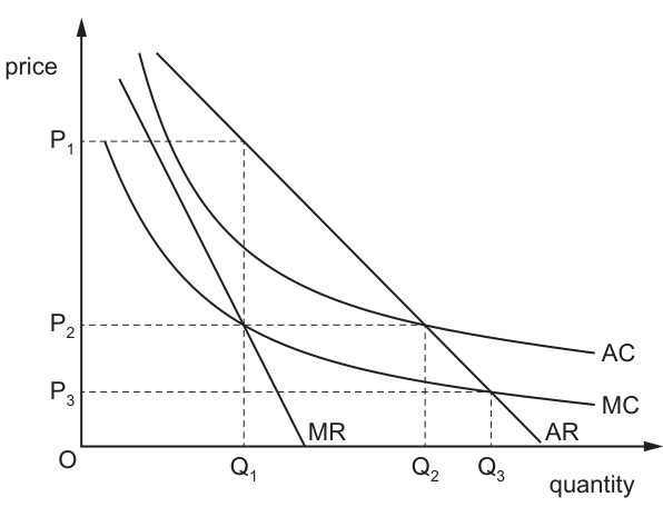
The diagram shows the cost and revenue curves for a natural monopoly.
Which statement is correct?
Options
A P2 and Q2 will achieve both allocative efficiency and productive efficiency.
B P2 and Q1 will achieve productive efficiency but not allocative efficiency.
C P3 and Q3 will achieve allocative efficiency but not productive efficiency.
D P3 and Q3 will achieve both allocative efficiency and productive efficiency.
Working
Allocative efficiency is achieved where price (P) equals marginal cost (MC), as this ensures the value consumers place on the final unit equals the cost of producing it. Productive efficiency is achieved at the output level where average cost (AC) is at its minimum, as this is the lowest possible cost per unit of output.
In the natural monopoly diagram:
- The point P3, Q3 is where the MC curve intersects the AR (demand) curve, so P = MC. This means P3, Q3 satisfies the condition for allocative efficiency.
- The AC curve is continuously falling over the relevant range of output (a defining feature of a natural monopoly, arising from economies of scale across the whole market demand), so Q3 is not at the minimum point of the AC curve. Therefore, P3, Q3 does not achieve productive efficiency.
Answer
C
C
Background Concept
A natural monopoly is a market structure where a single firm can supply the entire market at a lower cost than multiple competing firms. This occurs because the firm experiences economies of scale over the entire range of market demand: average costs (AC) fall continuously as output increases, so one large firm is more efficient than several smaller ones. On a cost and revenue diagram for a natural monopoly, the AC curve is continuously downward-sloping over the relevant output range, and the marginal cost (MC) curve lies below the AC curve (when MC is less than AC, average costs fall as output rises).
Two key efficiency concepts are tested in this question:
- Allocative efficiency: This is achieved when resources are allocated in a way that maximises total societal welfare. The formal condition for allocative efficiency is P = MC: the price consumers are willing to pay for the last unit (their marginal benefit) equals the marginal cost of producing that unit. At this point, no reallocation of resources can make one person better off without making another worse off (Pareto optimality).
- Productive efficiency: This is achieved when output is produced at the lowest possible cost per unit. The formal condition for productive efficiency is that output occurs at the minimum point of the average cost (AC) curve, as this is the point where average costs are lowest, and no resources are wasted in the production process.
For a monopoly, the average revenue (AR) curve is the firm's demand curve (downward-sloping, as the firm must lower price to sell more output), and the marginal revenue (MR) curve lies below the AR curve, also downward-sloping.
Understanding the Question
The question provides a diagram of a natural monopoly's cost and revenue curves, with three price-quantity combinations marked: (P1,Q1), (P2,Q2), (P3,Q3). It asks which statement correctly identifies which of these combinations achieves allocative efficiency, productive efficiency, both, or neither. The core task is to apply the formal definitions of the two efficiency types to the points on the diagram, and recognise the unique feature of a natural monopoly (continuously falling AC) that means the allocatively efficient point cannot be productively efficient.
Approach
First, state the formal conditions for allocative and productive efficiency to avoid confusion between the two. Then, locate each of the three marked points on the diagram and test them against the two conditions:
- First, identify the allocatively efficient point: this is where MC intersects the AR (demand) curve, as this is where P = MC.
- Next, check if this point is also productively efficient: this would require it to be at the minimum of the AC curve. For a natural monopoly, AC is continuously falling, so the minimum AC point is at a much higher output level than the market demand, meaning the allocatively efficient point will not be productively efficient.
- Check the other points to eliminate incorrect options: for example, (P2,Q2) is where AC = AR (the firm breaks even here), but P > MC so not allocatively efficient, and AC is still falling at Q2 so not productively efficient. (P1,Q1) is the unregulated monopoly profit-maximising point (MR=MC), which is neither allocatively nor productively efficient.
- Match the findings to the options to select the correct statement.
Step-by-Step Reasoning
-
Recall the efficiency conditions: These are the foundation of the question, so mixing them up is the most common source of error. Allocative efficiency requires P = MC (marginal benefit to consumers equals marginal cost of production), while productive efficiency requires output at the minimum of the AC curve (lowest possible cost per unit).
-
Analyse the natural monopoly diagram:
- A natural monopoly's AC curve falls continuously over the relevant output range because it enjoys economies of scale as it expands: spreading fixed costs over more units, and gaining purchasing or technical economies as output rises. This means MC lies below AC for all relevant output levels (when MC < AC, AC falls as output increases).
- The three marked points correspond to key monopoly outcomes:
- (P1, Q1): This is where MR = MC, the profit-maximising output and price for an unregulated monopoly. At this point, P1 > MC, so it is not allocatively efficient. AC is also higher at Q1 than at higher output levels, so it is not productively efficient.
- (P2, Q2): This is where AC = AR, meaning the firm earns normal profit (zero supernormal profit) at this output. At Q2, P2 > MC (since MC is below AC when AC is falling), so it is not allocatively efficient. AC is still falling at Q2 (as the AC curve is continuously downward-sloping), so Q2 is not the minimum AC point, meaning it is not productively efficient either.
- (P3, Q3): This is where MC intersects the AR (demand) curve, so P3 = MC. This exactly satisfies the allocative efficiency condition. However, AC is still falling at Q3 (the AC curve has not yet reached its minimum, which would occur at a much higher output level beyond the market demand for a natural monopoly), so Q3 is not at the minimum AC point. Therefore, P3, Q3 is allocatively efficient but not productively efficient.
-
Evaluate the options:
- Option A claims P2 and Q2 achieve both efficiencies. This is incorrect: P2 > MC so not allocatively efficient, and AC is still falling at Q2 so not productively efficient.
- Option B claims P2 and Q1 achieve productive but not allocative efficiency. This is incorrect for two reasons: first, Q1 is not the minimum AC point, so it is not productively efficient; second, P2 is not the price charged at Q1 (the price at Q1 is P1, from the AR curve), so (P2, Q1) is not a valid equilibrium point on the demand curve.
- Option C claims P3 and Q3 achieve allocative efficiency but not productive efficiency. This matches our analysis exactly: P3 = MC so allocatively efficient, but AC is still falling at Q3 so not productively efficient. This is the correct statement.
- Option D claims P3 and Q3 achieve both efficiencies. This is incorrect because productive efficiency requires minimum AC, which is not present at Q3.
Key Takeaways
- The two efficiency types have distinct, non-interchangeable conditions: never confuse P = MC (allocative) with P = AC or minimum AC (productive).
- For a natural monopoly, the continuously falling AC curve means the allocatively efficient output (P=MC) will always be productively inefficient, because productive efficiency would require producing at a much larger scale where AC is minimised, which is not feasible within the market demand. This is the core market failure associated with natural monopolies: the unregulated monopoly restricts output to raise price and profit, creating deadweight loss, while the allocatively efficient outcome would leave the firm making a loss (since P3 < AC at Q3), requiring regulation or subsidy to implement.
- When analysing monopoly diagrams, always first identify which curve is which (AR = demand, MR below AR, MC below AC when AC is falling) to avoid misreading points.
Common Mistakes
- Confusing efficiency conditions: A very common error is to assume that P = AC (the break-even point for the firm) is allocative efficiency, but allocative efficiency strictly requires P = MC. Another error is thinking any point on the AC curve is productively efficient, but only the minimum point of AC qualifies.
- Misidentifying diagram points: For example, assuming Q1 is the allocatively efficient point, but Q1 is where MR = MC (the unregulated monopoly profit-maximising point), not P = MC. Similarly, assuming (P2, Q1) is a valid point, but Q1 corresponds to price P1 on the AR curve, not P2, so this combination is not an equilibrium on the demand curve.
- Ignoring the natural monopoly feature: Forgetting that a natural monopoly has a continuously falling AC curve, so there is no minimum AC point in the relevant market range. This leads to the mistake of thinking Q2 or Q3 is the productively efficient point, when in fact productive efficiency would require a much higher output level.
- Failing to eliminate wrong options first: In multiple-choice questions, quickly eliminating obviously wrong options (like B, which uses an invalid price-quantity combination) saves time and reduces the chance of error.
Things to Be Careful About
- Always verify that a price-quantity combination lies on the AR (demand) curve: if the price does not match the AR curve at the given quantity, the point is not a valid market outcome, so any option using it is automatically wrong (as with option B's P2 and Q1).
- When checking for productive efficiency, confirm that the output is exactly at the minimum of the AC curve, not just that AC is lower than at other points. If AC is still falling, the minimum is at a higher output, so the current output is not productively efficient.
- The condition for allocative efficiency is exact equality of P and MC: do not accept "close to MC" as sufficient.
- For natural monopolies, remember that the falling AC curve means MC is always below AC, so P = MC (allocative efficiency) will always result in P < AC, meaning the firm makes a loss if unregulated, which is why natural monopolies are typically subject to price regulation.
What would not affect the budget line of an individual consumer?
Options
A the individual’s preference for various goods
B the level of income tax
C the money prices of goods
D the incomes earned by the individual
Reasoning
A budget line shows all combinations of two goods that a consumer can afford given their income and the prices of the goods. It is determined by the consumer's money income and the money prices of goods. A change in income tax affects disposable income, and a change in the individual's earned income also affects their budget. However, the individual's preferences for various goods determine which combination on the budget line they choose, not the position or slope of the budget line itself. Preferences affect the indifference map, not the budget constraint.
Answer
A
A
Background Concept
A budget line (or budget constraint) represents all the combinations of two goods that a consumer can purchase given their money income and the prices of the goods. Its equation is:
Px * Qx + Py * Qy = Income
where Px and Py are the prices of goods X and Y, and Qx and Qy are the quantities consumed. The slope of the budget line equals -Px/Py (the relative price ratio), and its position is determined by the level of income. Any change in money income or in the price of either good will shift or rotate the budget line.
An indifference curve, by contrast, shows all combinations of two goods that give the consumer the same level of satisfaction (utility). The shape of indifference curves reflects the consumer's preferences (their marginal rate of substitution between the goods). Preferences determine which point on the budget line the consumer chooses, but they do not affect the budget line itself.
Understanding the Question
The question asks: "What would not affect the budget line of an individual consumer?" Four options are given. The task is to identify the one factor that does NOT change the set of affordable combinations — i.e., does not shift or rotate the budget line. This is a straightforward test of the definition of a budget line and the distinction between the budget constraint (what you can afford) and preferences (what you want).
Approach
Recall the two determinants of a budget line: (1) the consumer's money income, and (2) the prices of the goods. Anything that changes either of these will affect the budget line. Anything that does not change either of these — such as a change in preferences — will not affect the budget line. Evaluate each option against this criterion.
Step-by-Step Reasoning
-
Option A: The individual's preference for various goods. Preferences determine the shape and position of indifference curves, not the budget line. A change in preferences means the consumer now values goods differently, so they will choose a different point on the same budget line, but the line itself — the set of affordable combinations — remains unchanged. Therefore, this does NOT affect the budget line.
-
Option B: The level of income tax. Income tax reduces the consumer's disposable income. A change in income tax changes the consumer's net income, which shifts the budget line inward (if tax rises) or outward (if tax falls). This DOES affect the budget line.
-
Option C: The money prices of goods. A change in the price of a good rotates the budget line (if one price changes) or shifts it (if both change proportionally). This directly affects the budget line.
-
Option D: The incomes earned by the individual. A change in earned income changes the consumer's total money income, shifting the budget line. This DOES affect the budget line.
Only option A is not a determinant of the budget line.
Key Takeaways
- The budget line is determined solely by income and prices. Preferences are irrelevant to its position or slope.
- A change in preferences changes the consumer's choice (the point on the budget line), not the budget line itself.
- This question tests the fundamental distinction between the budget constraint (what you can afford) and preferences (what you want).
Common Mistakes
- Confusing a movement along the budget line (caused by a change in preferences) with a shift of the budget line (caused by a change in income or prices).
- Thinking that a change in income tax is not a change in income — it is a change in disposable income, which is what matters for the budget line.
- Selecting option D because "incomes earned" might be confused with "income after tax" — but both affect the budget line.
Things to Be Careful About
- Read the question carefully: it asks for what would NOT affect the budget line. The correct answer is the exception.
- Remember that the budget line is a constraint, not a preference map. Preferences are captured by indifference curves, not the budget line.
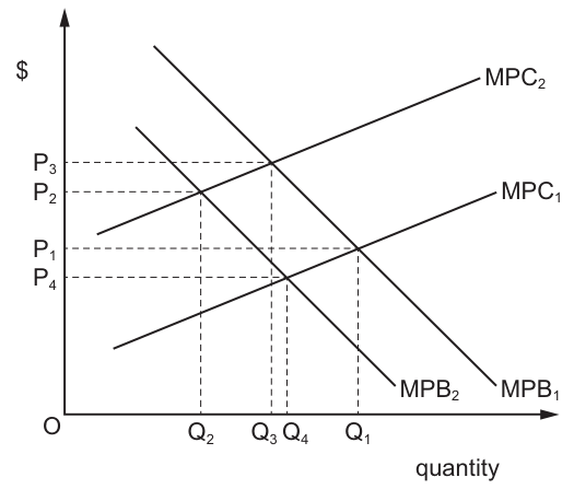
The diagram shows the marginal private costs (MPC) and marginal private benefits (MPB) of a product. Consumers initially estimate that marginal private costs are at MPC1 and marginal private benefits are at MPB1.
What is the impact on the market demand for the product if the consumer realises they have underestimated the MPC of buying the product but not the MPB?
Options
A The consumer underconsumes the product by Q1Q2.
B The consumer underconsumes the product by Q1Q3.
C The consumer overconsumes the product by Q1Q3.
D The consumer overconsumes the product by Q1Q4.
Working
The initial market equilibrium occurs where marginal private cost equals marginal private benefit, i.e. where MPC1 = MPB1. From the diagram, this intersection corresponds to quantity Q1.
When the consumer realises they have underestimated MPC, the actual marginal private cost is the higher curve MPC2, while MPB remains at MPB1. The new equilibrium is where MPC2 = MPB1, which corresponds to quantity Q3.
Since the original quantity consumed (Q1) is greater than the efficient quantity (Q3), the consumer has overconsumed the product by the difference Q1 - Q3 = Q1Q3.
Answer
C
C
Background Concept
Marginal private cost (MPC) is the additional cost incurred by a consumer when they consume one more unit of a good or service. Marginal private benefit (MPB) is the additional benefit a consumer gains from consuming one more unit of the same good. In the absence of externalities, the optimal consumption quantity for a consumer occurs where their MPC equals their MPB: at this point, the private cost of the last unit consumed exactly matches the private benefit it provides, so resources are allocated efficiently from the consumer's private perspective.
If a consumer misestimates their MPC, they will choose a consumption quantity that does not equate their actual MPC and MPB. Underestimating MPC means the consumer believes the cost of each additional unit is lower than it truly is, so they will consume more units than they would if they had accurate cost information. This leads to overconsumption: the quantity they actually consume is higher than the efficient quantity where actual MPC = MPB. The size of the overconsumption is the difference between the actual consumed quantity and the efficient quantity.
Understanding the Question
The question provides a diagram with two upward-sloping MPC curves (MPC1 and MPC2, where MPC2 lies to the left of MPC1, meaning it represents higher marginal costs at every quantity) and two downward-sloping MPB curves (MPB1 and MPB2, where MPB2 lies to the left of MPB1, meaning it represents lower marginal benefits at every quantity).
Initially, consumers believe their MPC is MPC1 and their MPB is MPB1, so their initial consumption equilibrium is at the intersection of these two curves, which corresponds to quantity Q1 on the horizontal axis.
The question asks for the impact on consumption if consumers realise they have underestimated their MPC (so the true MPC is the higher MPC2) but their estimate of MPB is correct (so MPB remains at MPB1). We need to find the new efficient equilibrium quantity, compare it to the original Q1, and determine the size and direction of the consumption gap.
Approach
- First, locate the initial equilibrium quantity: this is where the initially perceived MPC (MPC1) equals the perceived MPB (MPB1), read from the horizontal axis.
- Second, locate the revised efficient equilibrium quantity: this is where the actual MPC (MPC2, since MPC was underestimated) equals the unchanged MPB (MPB1), again read from the horizontal axis.
- Third, compare the two quantities: if the original quantity is larger than the revised efficient quantity, this is overconsumption; if smaller, underconsumption. The size of the gap is the absolute difference between the two quantities.
- Match this result to the four given options to select the correct answer.
Step-by-Step Reasoning
- Identify initial equilibrium: Consumers initially think their MPC is MPC1 and MPB is MPB1. The quantity they choose to consume is where their perceived marginal cost equals marginal benefit, which is the intersection of MPC1 and MPB1. From the diagram, this intersection aligns with quantity Q1 on the horizontal axis, so the initial quantity consumed is Q1.
- Identify the actual MPC: The consumer realises they underestimated MPC, meaning the true marginal cost of each unit is higher than MPC1. The diagram shows MPC2 is to the left of MPC1, so at every quantity, MPC2 > MPC1, which matches the scenario of an underestimated MPC. The MPB estimate is correct, so MPB does not shift and remains at MPB1.
- Identify the new efficient equilibrium: The efficient consumption quantity (where actual private costs equal private benefits) is now at the intersection of the actual MPC2 and the unchanged MPB1. From the diagram, this intersection aligns with quantity Q3 on the horizontal axis.
- Compare quantities and determine over/underconsumption: The original quantity consumed (Q1) is larger than the new efficient quantity (Q3). This means the consumer was consuming more than the optimal level, i.e. they overconsumed the product. The size of the overconsumption is the difference between the two quantities: Q1 - Q3 = Q1Q3.
- Match to options: This result matches option C, which states the consumer overconsumes by Q1Q3.
Key Takeaways
- The optimal consumption quantity for a consumer occurs where their marginal private cost (MPC) equals their marginal private benefit (MPB). Any deviation from this equality leads to over or underconsumption.
- Underestimating MPC leads to overconsumption, because the consumer believes additional units are cheaper than they really are, so they buy more than the efficient quantity. Overestimating MPC would lead to underconsumption.
- When analysing diagrams of MPC and MPB, always match the intersection of the relevant curves to the horizontal axis to find the equilibrium quantity, and compare quantities to calculate the size of any consumption gap.
- For multiple-choice questions involving diagram interpretation, first eliminate obviously wrong options (here, options A and B mention underconsumption, which is incorrect because underestimated MPC leads to higher consumption than efficient, so overconsumption) before calculating the exact gap to choose between the remaining options.
Common Mistakes
- Confusing MPC and MPB curves: MPC is upward-sloping (costs rise as more units are consumed), while MPB is downward-sloping (benefits fall as more units are consumed). Mixing these up will lead to identifying the wrong intersection points and an incorrect answer.
- Mixing up overconsumption and underconsumption: Underestimating MPC means the consumer thinks costs are lower than they are, so they consume more than the efficient quantity, which is overconsumption, not underconsumption. This eliminates options A and B immediately.
- Using the wrong curve intersections: The question specifies that MPB is not underestimated, so MPB stays at MPB1. Do not use the intersection of MPC2 and MPB2 (which would be Q2) or MPC1 and MPB2 (which would be Q4), as these do not match the scenario.
- Misreading the quantity gap: The gap is Q1Q3, not Q1Q2 or Q1Q4. Q1Q2 is the gap between the initial equilibrium and the intersection of MPC2 and MPB2, which is irrelevant because MPB did not change. Q1Q4 is the gap between the initial equilibrium and MPC1 with MPB2, which is also irrelevant.
Things to Be Careful About
- Always confirm which curves have shifted: in this scenario, only MPC shifts from MPC1 to MPC2 (higher costs), MPB remains unchanged at MPB1. Any option that relies on a shift in MPB is incorrect.
- When calculating the size of the consumption gap, subtract the smaller efficient quantity from the larger original quantity: Q1 (original) minus Q3 (efficient) equals Q1Q3, which is the overconsumption gap.
- The direction of the MPC shift matters: an underestimated MPC means the actual MPC curve is to the left of the estimated one (higher costs at each quantity), leading to a lower equilibrium quantity. If MPC were overestimated (actual MPC to the right of estimated), the equilibrium quantity would be higher, leading to underconsumption.
- Ensure you read the intersection points correctly: the dashed lines in the diagram link each intersection to its corresponding price and quantity, so follow the dashed line from the relevant intersection down to the horizontal axis to get the correct quantity value.
What is an internal economy of scale?
Options
A efficient local transport networks
B improved access to spare parts as a result of industry growth
C lower risks from supplying a wider range of customers
D the training of skilled labour at a college financed by local firms
Answer
Internal economies of scale are cost advantages that arise from the growth of the firm itself, such as technical, managerial, financial, marketing, and risk-bearing economies. Option C describes lower risks from supplying a wider range of customers, which is a risk-bearing internal economy of scale. Options A, B, and D describe external economies of scale that benefit all firms in the industry.
Answer
C
C
Background Concept
Economies of scale refer to the cost advantages that firms experience when output increases. These can be internal or external. Internal economies of scale are cost savings that accrue to a firm as it expands its own scale of operations. They include technical economies (e.g., using larger, more efficient machinery), managerial economies (specialisation of management), financial economies (better borrowing terms), marketing economies (bulk advertising), and risk-bearing economies (diversification of products or customers). External economies of scale are cost reductions that benefit all firms in an industry as the industry grows, such as improved infrastructure, a pool of skilled labour, or specialised suppliers.
Understanding the Question
This is a multiple-choice question that tests the distinction between internal and external economies of scale. The question asks: 'What is an internal economy of scale?' and provides four options. The correct answer is the one that describes a cost advantage arising from the firm's own growth, not from the growth of the industry as a whole.
Approach
Recall the definition of internal economies of scale and evaluate each option against that definition. Eliminate options that describe external economies of scale.
Step-by-Step Reasoning
- Option A: 'efficient local transport networks' – This is an external economy because improved transport benefits all firms in the area, not just one firm. It arises from the growth of the local economy or industry, not from the expansion of a single firm.
- Option B: 'improved access to spare parts as a result of industry growth' – This is also an external economy. As the industry grows, suppliers become more specialised and efficient, benefiting all firms. The cost advantage comes from industry-wide expansion.
- Option C: 'lower risks from supplying a wider range of customers' – This is an internal economy of scale. When a firm grows and diversifies its customer base, it reduces its dependence on any single customer, lowering the risk of revenue loss. This is a risk-bearing internal economy that results from the firm's own expansion.
- Option D: 'the training of skilled labour at a college financed by local firms' – This is an external economy. The college is funded collectively by local firms, creating a pool of trained workers that benefits all firms in the industry. The cost of training is shared, and the benefit is external to any single firm.
Therefore, the correct answer is C.
Key Takeaways
- Internal economies of scale arise from the growth of the firm itself; external economies arise from the growth of the industry.
- Examples of internal economies: technical, managerial, financial, marketing, risk-bearing.
- Examples of external economies: improved infrastructure, specialised labour pools, supplier networks.
Common Mistakes
- Confusing internal and external economies: students often mistake industry-wide benefits (like better transport) as internal because they reduce costs for the firm, but they are external because they do not depend on the firm's own size.
- Overlooking risk-bearing economies: risk-bearing is a less obvious internal economy, but it is a valid one when the firm diversifies its customer base or product range.
Things to Be Careful About
- Read each option carefully and identify whether the cost advantage is due to the firm's own expansion or the industry's expansion.
- Remember that internal economies are specific to the firm and its scale; external economies are shared by all firms in the industry.
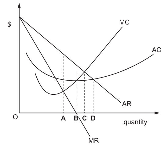
The diagram shows the costs and revenue for a monopoly.
Which level of output would produce only a normal profit?
Options
A output level A on Fig. 6.1
B output level B on Fig. 6.1
C output level C on Fig. 6.1
D output level D on Fig. 6.1
Reasoning
Normal profit occurs where a firm's total revenue equals its total cost, so economic profit is zero. This break-even point arises where average revenue (AR, equal to price for a monopoly) equals average total cost (AC). On the provided diagram, this condition is met at output level D, where the AR and AC curves intersect. At outputs A, B and C, AR is above AC, so the firm would earn supernormal profit at these levels.
Answer
D
D
Background Concept
Profit for any firm is calculated as total revenue (TR) minus total cost (TC). Economists distinguish between three types of profit:
- Supernormal profit (economic profit): TR > TC, meaning the firm earns more than the minimum required to keep its resources in their current use. This is the profit above normal profit.
- Normal profit: TR = TC, so economic profit is zero. This is the minimum profit needed to keep the firm operating in the long run, as it covers all explicit costs (payments to external suppliers) and implicit costs (the opportunity cost of the owner's time and capital). Normal profit is treated as a cost of production and is included in the firm's average total cost (AC) curve.
- Subnormal profit (loss): TR < TC, so the firm is not covering all its costs, including normal profit.
For any firm, average revenue (AR) is equal to price, and is calculated as TR divided by output quantity. Average total cost (AC) is TC divided by output quantity. Therefore, the condition TR = TC (normal profit) is equivalent to AR = AC. This is the break-even point for the firm.
In a monopoly, the firm faces a downward-sloping demand curve, so its AR curve is also downward-sloping. The marginal revenue (MR) curve lies below the AR curve because the firm must lower price for all units to sell more output, so each additional unit adds less to total revenue than the price charged. The marginal cost (MC) curve is upward-sloping in the short run due to the law of diminishing marginal returns, and the AC curve is U-shaped because MC intersects AC at its minimum point: when MC is below AC, AC falls; when MC is above AC, AC rises.
Understanding the Question
The question provides a cost and revenue diagram for a monopoly and asks which output level produces only a normal profit. The diagram marks four output levels: A (MC = MR), B (minimum AC), C (MC = AR), and D (AR = AC). The task is to apply the definition of normal profit to the diagram to select the correct option. The key challenge is to avoid confusing the normal profit point with other common intersections on the monopoly diagram, such as the profit-maximising output (MC = MR) or the allocatively efficient output (MC = AR).
Approach
To solve this, follow these steps:
- Recall the definition of normal profit and its condition: normal profit occurs where TR = TC, which is equivalent to AR = AC (the break-even point).
- Identify what each marked output level represents on the diagram:
- Output A: Intersection of MC and MR → the monopoly's profit-maximising output.
- Output B: Minimum point of the AC curve → productive efficiency.
- Output C: Intersection of MC and AR → allocative efficiency.
- Output D: Intersection of AR and AC → break-even point.
- Compare the AR and AC values at each output to determine the profit level:
- If AR > AC: supernormal profit.
- If AR = AC: normal profit.
- If AR < AC: subnormal profit.
- Select the output level that meets the normal profit condition.
Step-by-Step Reasoning
- Define normal profit: Normal profit is the minimum profit required to keep a firm in its current industry in the long run. It covers all explicit costs (e.g., wages, rent, materials) and implicit costs (the opportunity cost of the owner's resources). Since normal profit is a cost of production, it is included in the firm's average total cost (AC) curve. When a firm earns only normal profit, its total revenue (TR) equals total cost (TC), so economic (supernormal) profit is zero.
- Link to the diagram: AR is equal to price for a monopoly, and is calculated as TR divided by output quantity. AC is TC divided by output quantity. Therefore, AR = AC is exactly the condition for TR = TC, or normal profit. The output level where the AR and AC curves intersect is the break-even point.
- Analyse each output level:
- Output A (MC = MR): This is the profit-maximising rule for all firms, including monopolies. At this output, the AR curve lies above the AC curve, so TR > TC, and the firm earns supernormal profit. This is not normal profit.
- Output B (minimum AC): This is the point of productive efficiency, where the firm produces at the lowest possible average cost. However, at this output, the AR curve is still above the AC curve, so TR > TC, and the firm earns supernormal profit.
- Output C (MC = AR): This is the allocatively efficient output, where the price consumers pay equals the marginal cost of production, maximising total social surplus. At this output, MC is above AC (since MC crosses AC at its minimum point B, and is rising for all outputs above B). Since AR = MC at C, this means AR = MC > AC, so AR > AC, and the firm earns supernormal profit.
- Output D (AR = AC): At this output, the AR and AC curves intersect, so AR = AC. This means TR = TC, so the firm earns only normal profit (zero economic profit). This matches the question's requirement.
- Conclusion: Output level D is the only level that produces only a normal profit.
Key Takeaways
- Normal profit is zero economic profit, occurring where AR = AC (the break-even point). It is not a separate type of profit added to AC, but is already included in the AC curve as an implicit cost.
- The profit-maximising output for a monopoly (MC = MR) always earns supernormal profit because the downward-sloping AR curve lies above the AC curve at that output (due to barriers to entry preventing competition from eroding profits).
- Allocative efficiency (MC = AR) is a separate concept from normal profit; it only coincides with the break-even point if MC = AC at that output, which only occurs at the minimum of the AC curve.
- To identify profit levels on a cost and revenue diagram, always compare the position of the AR curve relative to the AC curve: AR above AC = supernormal, AR equal to AC = normal, AR below AC = subnormal.
Common Mistakes
- Confusing the profit-maximising output (MC = MR) with the normal profit point: Many students assume the monopoly's profit-maximising output is the normal profit point, but this is incorrect because the monopoly sets output where MR = MC, which is always to the left of the AR = AC intersection, leading to supernormal profit.
- Mixing up allocative efficiency (MC = AR) with normal profit: Allocative efficiency is about social welfare, not the firm's profit level. At the allocatively efficient output, the firm may still earn supernormal profit if AR > AC.
- Misidentifying curve intersections: Failing to correctly distinguish between AR, MR, MC and AC curves leads to selecting the wrong output. Remember that for a monopoly, AR is the flatter downward-sloping curve, MR is the steeper downward-sloping curve, MC is upward-sloping, and AC is U-shaped.
- Assuming the minimum of AC is the normal profit point: The minimum of AC is only the normal profit point if AR also equals AC at that output, which is not the case in this diagram.
Things to Be Careful About
- Always verify which curves intersect at each marked output level: For normal profit, confirm the intersection is between AR and AC, not other curves.
- Remember that normal profit is included in AC: Do not treat normal profit as an extra amount on top of AC; it is already part of the AC curve, so AR = AC is the correct condition.
- Check the relative positions of AR and AC at each output: If AR is above AC, profit is supernormal; if equal, normal; if below, subnormal.
- In this diagram, the AC curve is below AR at outputs A, B and C, so only at D (where they intersect) is profit normal. At outputs beyond D, AC would be above AR, leading to subnormal profit.
Which combination of statements about small firms and large firms is most likely to be correct?
Options
| small firms | large firms | |
|---|---|---|
| A | are more common in manufacturing than in services | face high barriers to exit |
| B | are more numerous than large firms | do not experience diseconomies of scale |
| C | can do well when each item produced is different | may arise from internal growth or mergers |
| D | cannot have any monopoly power | cannot earn supernormal profits |
Reasoning
Small firms are more numerous than large firms in most economies, but they do experience diseconomies of scale beyond a certain size. Large firms can arise from internal growth (organic expansion) or external growth (mergers and takeovers). Option C correctly states that small firms can do well when each item produced is different (e.g., customised products or niche markets) and that large firms may arise from internal growth or mergers.
Option A is incorrect because small firms are more common in services than in manufacturing. Option B is incorrect because large firms can and do experience diseconomies of scale. Option D is incorrect because small firms can have monopoly power in a local market, and large firms can earn supernormal profits.
Answer
C
C
Background Concept
Firms vary greatly in size, from sole traders to multinational corporations. The reasons for these differences include economies of scale, barriers to entry, market structure, and the nature of the product. Small firms are often more flexible and can cater to niche markets, while large firms benefit from mass production and market power. However, large firms may suffer from diseconomies of scale (e.g., coordination problems), and small firms can still have monopoly power in a localised market.
Understanding the Question
This question asks you to identify which combination of statements about small firms and large firms is most likely to be correct. Each option pairs a claim about small firms with a claim about large firms. You need to evaluate each pair and select the one where both statements are true.
Approach
Go through each option one by one, checking the truth of both statements. Use your knowledge of firm size, market structure, economies of scale, and growth strategies. Eliminate any option where at least one statement is false.
Step-by-Step Reasoning
-
Option A: "Small firms are more common in manufacturing than in services" – This is false. Small firms are actually more common in the service sector (e.g., hairdressers, cafes, consultants) because manufacturing often requires large capital investment. "Large firms face high barriers to exit" – This is generally false; large firms may face some exit costs but not necessarily high barriers. So A is incorrect.
-
Option B: "Small firms are more numerous than large firms" – This is true. In most economies, the vast majority of firms are small. "Large firms do not experience diseconomies of scale" – This is false. Large firms often experience diseconomies of scale (e.g., communication problems, bureaucracy). So B is incorrect.
-
Option C: "Small firms can do well when each item produced is different" – This is true. Small firms can thrive in niche markets where customisation is important (e.g., bespoke tailoring, specialist engineering). "Large firms may arise from internal growth or mergers" – This is true. Large firms can grow organically (internal growth) or through mergers and takeovers (external growth). So C is correct.
-
Option D: "Small firms cannot have any monopoly power" – This is false. A small firm can have monopoly power in a local market (e.g., the only petrol station in a remote village). "Large firms cannot earn supernormal profits" – This is false. Large firms with market power (e.g., monopolies or oligopolies) can earn supernormal profits. So D is incorrect.
Therefore, the correct answer is C.
Key Takeaways
- Small firms are more numerous and often serve niche or customised markets.
- Large firms can grow internally or externally, but they are not immune to diseconomies of scale.
- Monopoly power is not exclusive to large firms; small firms can have local monopoly power.
- Supernormal profits are possible for firms with market power, regardless of size.
Common Mistakes
- Assuming that small firms cannot have any market power – they can in local markets.
- Thinking that large firms never experience diseconomies of scale – they often do.
- Confusing the prevalence of small firms in manufacturing vs. services.
Things to Be Careful About
- Read each statement carefully; both parts of the pair must be true.
- Remember that "most likely to be correct" means the pair with the highest probability of being true, not a perfect statement.
- Use elimination to narrow down options.
Good X is a popular product that creates a negative externality when it is consumed.
The government wants to reduce the consumption of good X significantly.
Under which circumstances is the government most likely to meet its aim?
Options
| government policy | price elasticity of demand for good X | |
|---|---|---|
| A | subsidy | more than 1 |
| B | subsidy | less than 1 |
| C | indirect tax | more than 1 |
| D | indirect tax | less than 1 |
Reasoning
A subsidy would lower the price and increase consumption, which is the opposite of the government's aim. Therefore, only an indirect tax is appropriate. To reduce consumption significantly, demand must be price elastic (PED > 1) so that the price rise leads to a more than proportionate fall in quantity demanded. Hence, the correct combination is indirect tax with PED > 1.
Answer
C
C
Background Concept
Good X creates a negative externality in consumption, meaning its consumption imposes external costs on third parties not reflected in the market price. This leads to overconsumption relative to the socially optimal level. Governments can intervene to correct this market failure. A common policy is to impose an indirect tax (a Pigouvian tax) on the good, which increases its price and reduces quantity demanded. The effectiveness of such a tax in reducing consumption depends on the price elasticity of demand (PED). PED measures the responsiveness of quantity demanded to a change in price. If demand is elastic (PED > 1), a given percentage price increase leads to a larger percentage decrease in quantity demanded. If demand is inelastic (PED < 1), the quantity decrease is proportionally smaller.
Understanding the Question
The question presents a scenario where the government wants to significantly reduce consumption of a good that has a negative externality. It asks under which combination of government policy (subsidy or indirect tax) and price elasticity of demand (more than 1 or less than 1) the government is most likely to achieve its aim. The key is to recognise that a subsidy would lower the price and encourage more consumption, making it counterproductive. Therefore, only an indirect tax is viable. Then, to achieve a significant reduction, the demand must be elastic so that the tax causes a large fall in quantity.
Approach
First, rule out the subsidy option because it would increase consumption, not reduce it. Then, for the indirect tax, consider the effect of elasticity: with elastic demand, the quantity falls more than the price rises, leading to a large reduction; with inelastic demand, the quantity falls only slightly. The question asks for the scenario most likely to meet the aim of significant reduction, so we choose elastic demand. Thus, the correct answer is C: indirect tax with PED > 1.
Step-by-Step Reasoning
- Identify the problem: Good X has a negative externality in consumption, so the market overconsumes it. The government wants to reduce consumption significantly.
- Evaluate policy options:
- Subsidy: A subsidy lowers the price paid by consumers, increasing quantity demanded. This would worsen the overconsumption, so it is not suitable.
- Indirect tax: An indirect tax raises the price paid by consumers, decreasing quantity demanded. This is appropriate to reduce consumption.
- Consider elasticity:
- If demand is elastic (PED > 1), the percentage change in quantity demanded is greater than the percentage change in price. So a tax that raises price by, say, 10% would reduce quantity by more than 10%, achieving a significant reduction.
- If demand is inelastic (PED < 1), the percentage change in quantity is smaller than the percentage change in price. A 10% price rise might reduce quantity by only 2%, which is not a significant reduction.
- Conclusion: The combination that most likely meets the aim is an indirect tax with elastic demand. This corresponds to option C.
Key Takeaways
- To correct a negative externality in consumption, a tax (Pigouvian tax) is appropriate; a subsidy would be counterproductive.
- The effectiveness of a tax in reducing consumption depends on the price elasticity of demand: the more elastic the demand, the greater the reduction in quantity for a given tax.
- When a question asks for the scenario most likely to achieve a significant reduction, consider both the direction of the policy and the magnitude of the response.
Common Mistakes
- Choosing a subsidy because it is often associated with positive externalities; here it would increase consumption, not reduce it.
- Confusing elastic and inelastic: thinking that inelastic demand leads to a large reduction (it actually leads to a small reduction in quantity but a large increase in government revenue).
- Not reading the question carefully: the aim is to reduce consumption significantly, so the combination that gives the largest reduction is needed.
Things to Be Careful About
- Always consider the direction of the policy: a subsidy lowers price, a tax raises price.
- Remember that price elasticity of demand is defined as the absolute value of the percentage change in quantity divided by the percentage change in price. For a tax, the price rises, so quantity falls; the elasticity determines how much.
- The question is multiple choice, so eliminate obviously wrong options first (subsidy options A and B) and then choose between C and D based on elasticity.
A government introduces tradeable pollution permits to reduce pollution.
What is an advantage of this scheme?
Options
A It allows consumers to determine the optimum pollution level.
B It can provide rewards for firms that reduce pollution.
C It enables the government to raise revenue from the resale of permits.
D It uses the market system with no administrative costs.
Reasoning
Tradeable pollution permits work by setting a cap on total emissions and issuing permits equal to that cap. Firms that reduce their pollution below their permit allocation can sell their surplus permits to other firms. This creates a financial reward for cutting pollution — the firm gains revenue from the permit sale — which is the scheme's core incentive mechanism.
Option A is incorrect because the government, not consumers, sets the total cap (the optimum pollution level). Option C is incorrect because the government raises revenue from the initial auction or allocation of permits, not from their resale between firms. Option D is incorrect because the scheme involves administrative costs for monitoring, enforcement, and running the permit market.
Answer
B
B
Background Concept
Tradeable pollution permits (also called cap-and-trade) are a market-based policy to correct the negative externality of pollution. The government sets a maximum allowable level of pollution (the cap) and issues permits equal to that cap. Each permit gives a firm the right to emit a specified amount of pollution. Firms can buy and sell these permits among themselves. The key economic idea is that firms with low abatement costs will reduce pollution more and sell their spare permits, while firms with high abatement costs will buy permits rather than cut pollution. This achieves the pollution target at the lowest possible total cost to society.
Understanding the Question
This is a multiple-choice question asking for the single advantage of a tradeable pollution permit scheme. The four options present different claims about what the scheme does. The task is to identify which one is genuinely an advantage of the scheme, as opposed to a misunderstanding or a feature that is not actually an advantage.
Approach
Read each option carefully and evaluate it against the standard economic analysis of tradeable permits. Option B describes the core incentive: firms that reduce pollution can sell permits and earn revenue. This is a genuine advantage because it rewards pollution reduction. The other options contain errors: A confuses who sets the cap, C confuses the source of government revenue, and D ignores the real administrative costs.
Step-by-Step Reasoning
Option A: "It allows consumers to determine the optimum pollution level."
- The optimum pollution level is determined by the government when it sets the cap. The government decides how many permits to issue based on its assessment of the marginal social cost and marginal social benefit of pollution. Consumers do not directly determine this level. So A is false.
Option B: "It can provide rewards for firms that reduce pollution."
- This is correct. If a firm reduces its pollution below the number of permits it holds, it can sell the surplus permits to another firm. The revenue from that sale is a direct financial reward for cutting pollution. This is the key advantage of a market-based system: it creates a price signal that incentivises firms to find the cheapest ways to reduce emissions.
Option C: "It enables the government to raise revenue from the resale of permits."
- The government raises revenue when it initially auctions permits to firms. However, the resale of permits happens between firms, not back to the government. The government does not earn revenue from the secondary market. So C is false.
Option D: "It uses the market system with no administrative costs."
- While the scheme does use market forces, it still requires administrative costs: monitoring emissions, enforcing the cap, running the permit registry, and policing fraud. These costs are not zero. So D is false.
Therefore, only B is a correct statement of an advantage.
Key Takeaways
- Tradeable permits create a financial incentive for firms to reduce pollution by allowing them to sell surplus permits.
- The government sets the cap, not consumers.
- Government revenue comes from the initial auction, not from resale.
- Administrative costs exist for monitoring and enforcement.
Common Mistakes
- Confusing the initial auction revenue with revenue from resale (option C).
- Assuming that a market-based system has zero administrative costs (option D).
- Thinking that consumers determine the pollution level (option A).
Things to Be Careful About
- Read each option precisely. Option B says "can provide rewards" — it does not claim that all firms will be rewarded, only that the scheme makes it possible.
- Remember that the advantage of tradeable permits is their cost-effectiveness in achieving a given pollution target, not the absence of costs or the source of government revenue.
To reduce traffic congestion, a government built a new highway. A majority of the citizens were opposed to this. Some citizens responded by switching from public transport to private cars. This caused car journeys to take even longer.
What can be concluded about government failure in this case?
Options
A It occurred because the government‘s opportunity costs were not considered.
B It occurred because the wishes of the majority of citizens were ignored.
C It occurred because the result was unintended.
D It occurred from over-reliance on the market system.
Reasoning
Government failure occurs when government intervention in the economy leads to a net welfare loss, often because the outcome is worse than the original problem or because the intervention produces unintended and undesirable side effects. In this case, the government built a new highway to reduce congestion, but the policy backfired: citizens switched from public transport to private cars, making journeys even longer. The result was directly contrary to the intended aim. This is a classic example of government failure caused by an unintended consequence of the policy.
Option A is incorrect because the scenario does not mention opportunity cost as the reason for failure. Option B is incorrect because government failure is an economic concept about welfare loss, not about ignoring democratic wishes. Option D is incorrect because the government intervened directly (building a highway), not by relying on the market.
Answer
C
C
Background Concept
Government failure occurs when government intervention in a market leads to a net loss of economic welfare, making the situation worse than the original market failure. It can arise from several causes:
- Unintended consequences: policies produce outcomes the government did not foresee or intend.
- Information failure: the government lacks the information needed to design an effective policy.
- Bureaucratic inefficiency: government agencies may not have the same incentives as private firms to minimise costs.
- Regulatory capture: regulators act in the interests of the firms they regulate rather than the public.
- Political self-interest: politicians may pursue policies that maximise votes rather than welfare.
- Ignoring external costs or benefits: the policy may create new externalities.
In this question, the key is to identify which of these causes is illustrated by the specific scenario.
Understanding the Question
The question describes a government building a new highway to reduce traffic congestion. The majority of citizens opposed the project. After the highway opened, some citizens switched from public transport to private cars, which made car journeys even longer than before. The question asks what can be concluded about government failure in this case, and provides four possible explanations.
We need to match the scenario to the correct definition of government failure. The key fact is that the policy produced an outcome opposite to its intended aim (reducing congestion actually increased journey times). This is a textbook example of an unintended consequence.
Approach
- Read the scenario carefully and identify the outcome: the policy made the problem worse.
- Recall the definition of government failure and its common causes.
- Evaluate each option against the scenario:
- Option A: opportunity cost not considered — not mentioned or implied.
- Option B: wishes of the majority ignored — this is a political or democratic failure, not necessarily an economic one.
- Option C: unintended result — matches the outcome exactly.
- Option D: over-reliance on the market system — the government intervened directly, not via the market.
- Select the option that best fits the economic concept.
Step-by-Step Reasoning
Step 1: Identify the intended outcome.
The government wanted to reduce traffic congestion.
Step 2: Identify the actual outcome.
Car journeys took even longer than before. Congestion worsened.
Step 3: Identify the mechanism.
The new highway induced some citizens to switch from public transport to private cars. This increased the number of cars on the road, offsetting any capacity gain from the new highway and making congestion worse.
Step 4: Classify the failure.
The government did not anticipate this behavioural response. The policy produced an outcome that was not intended and was worse than the original problem. This is government failure due to unintended consequences.
Step 5: Evaluate each option.
-
Option A: "It occurred because the government's opportunity costs were not considered." Opportunity cost is the value of the next best alternative forgone. While building the highway had an opportunity cost (e.g., the money could have been spent on improving public transport), the scenario does not suggest that ignoring this cost was the cause of the failure. The failure was not about the cost of the project but about its perverse effect. So A is incorrect.
-
Option B: "It occurred because the wishes of the majority of citizens were ignored." The majority opposed the highway, but government failure is an economic concept about welfare loss, not about democracy. A policy can be popular and still cause government failure, or unpopular and still be efficient. Ignoring the majority's wishes is a political issue, not necessarily an economic failure. So B is incorrect.
-
Option C: "It occurred because the result was unintended." This is exactly what happened. The government intended to reduce congestion but instead made it worse. The outcome was unintended and undesirable. This is a classic cause of government failure. So C is correct.
-
Option D: "It occurred from over-reliance on the market system." The government did not rely on the market; it directly provided a public good (the highway). Over-reliance on the market would mean the government left the problem to the private sector, which is the opposite of what happened. So D is incorrect.
Step 6: Conclude.
The correct answer is C.
Key Takeaways
- Government failure is not simply "the government made a mistake" — it is a specific economic concept where intervention reduces net welfare.
- Unintended consequences are a common cause of government failure, especially when policies change incentives in ways policymakers did not foresee.
- In multiple-choice questions, match the scenario to the precise definition, not to a plausible-sounding but incorrect option.
- Distinguish between economic failure (welfare loss) and political failure (ignoring public opinion).
Common Mistakes
- Choosing Option B because it sounds like "the government ignored the people" — but the question asks about government failure in an economic sense, not a democratic one.
- Choosing Option A because "opportunity cost" is a familiar term — but the scenario does not provide any information about what was forgone or whether that was the cause of the failure.
- Confusing government failure with market failure: Option D describes a market failure (over-reliance on the market), but the government intervened, so this is not applicable.
Things to Be Careful About
- Read the question carefully: it asks what can be concluded about government failure in this case. The answer must be directly supported by the scenario.
- Do not overthink: the scenario is a textbook example of unintended consequences. The simplest correct answer is often the right one.
- Remember that government failure can occur even when the government acts with good intentions — the outcome matters, not the motive.
What could result in an individual being caught in the poverty trap if their income increases?
Options
A national minimum wage is changed
B benefits payments are means-tested
C subsidised housing payments for low-income earners are increased
D the income level at which income tax is first paid is increased
Answer
The poverty trap occurs when an increase in gross income leads to a reduction in means-tested benefits, so that net income rises by little or nothing. Option B directly describes this: benefits payments that are means-tested are withdrawn as income rises, creating a high effective marginal tax rate that traps individuals in poverty.
Answer
B
B
Background Concept
The poverty trap is a situation where individuals or households have little or no net financial gain from increasing their earned income, because the increase is offset by the withdrawal of means-tested benefits and/or an increase in tax liabilities. The effective marginal tax rate — the proportion of each additional unit of earned income that is lost to higher taxes and reduced benefits — can approach or even exceed 100%, removing the financial incentive to work more or seek higher pay.
Means-tested benefits are payments (e.g., housing benefit, income support, tax credits) that are reduced as the recipient's income rises. They are designed to target support at the poorest, but the withdrawal rate creates the poverty trap.
Understanding the Question
The question asks which of four policy changes could result in an individual being caught in the poverty trap if their income increases. The key is to identify the option that creates or worsens the disincentive effect — where a rise in gross income leads to little or no rise in net income.
Approach
Evaluate each option in turn:
- A: Changing the national minimum wage affects gross pay, not the withdrawal of benefits. It could lift someone out of poverty but does not itself create a trap.
- B: Means-tested benefits are the classic cause of the poverty trap. If benefits are withdrawn as income rises, net income may not increase much.
- C: Increasing subsidised housing payments for low-income earners is a benefit increase, but the trap depends on the withdrawal rate, not the level. A higher subsidy could actually reduce the trap if it is not withdrawn quickly, but the question asks what could result in being caught — and increasing a means-tested benefit without changing the taper rate still leaves the trap in place.
- D: Raising the income tax threshold reduces the tax burden on low earners, which reduces the poverty trap by lowering the effective marginal tax rate.
Only option B directly describes the mechanism that creates the trap.
Step-by-Step Reasoning
-
Define the poverty trap: When an individual's gross income rises, their net income (after tax and benefits) rises by less than the gross increase, or may even fall, because benefits are withdrawn and/or taxes increase.
-
Analyse option B: Means-tested benefits are explicitly reduced as income rises. For example, if a benefit is withdrawn at a rate of 50p for every £1 earned, then a £100 gross pay rise leads to a £50 benefit cut, so net income rises by only £50. If the withdrawal rate is 100%, net income does not rise at all. This is the textbook cause of the poverty trap.
-
Analyse option A: Changing the national minimum wage alters the wage floor. A higher minimum wage raises gross pay for low earners, which could lift them out of poverty. It does not, by itself, create a trap — the trap arises from the interaction of earnings with the benefit and tax system.
-
Analyse option C: Increasing subsidised housing payments for low-income earners raises the level of a means-tested benefit. If the benefit is withdrawn as income rises, the trap remains. However, the question asks what could result in being caught — and the existence of means-testing (option B) is the direct cause. A higher benefit level without changing the taper does not create the trap; it is the withdrawal that does.
-
Analyse option D: Raising the income tax threshold means that low earners pay less tax on their additional earnings. This reduces the effective marginal tax rate, making work more rewarding and alleviating the poverty trap.
-
Conclusion: Only option B describes a policy that directly creates or perpetuates the poverty trap.
Key Takeaways
- The poverty trap is caused by the withdrawal of means-tested benefits and/or increases in tax as income rises.
- The effective marginal tax rate is the key measure: the proportion of extra gross income lost to higher taxes and lower benefits.
- Policies that reduce the withdrawal rate (e.g., lowering taper rates, raising tax thresholds) alleviate the trap; policies that introduce or maintain means-testing perpetuate it.
Common Mistakes
- Confusing the poverty trap with low income itself. The trap is about the disincentive to increase income, not about being poor.
- Thinking that increasing benefits (option C) always helps. If the benefit is means-tested, the trap remains; the level of the benefit does not change the withdrawal mechanism.
- Assuming that raising the minimum wage (option A) creates a trap. It raises gross pay, which is separate from the benefit/tax interaction.
Things to Be Careful About
- Read the question carefully: it asks what could result in being caught in the trap, not what is a policy to reduce poverty.
- Distinguish between the level of a benefit and the withdrawal rate. The trap is about the rate, not the level.
- Remember that the poverty trap is a microeconomic concept about individual incentives, not a macroeconomic phenomenon.
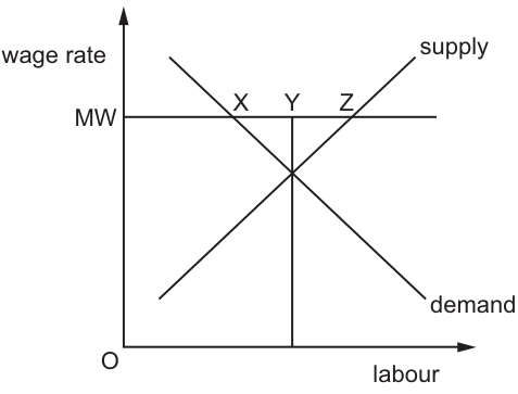
The diagram shows the impact on the labour market of the introduction of a national minimum wage (MW).
What do the distances XY and YZ represent?
Options
| XY | YZ | |
|---|---|---|
| A | increase in employed workers | existing workers made redundant |
| B | existing workers made redundant | unemployed new entrants |
| C | existing workers made redundant | increase in employed workers |
| D | unemployed new entrants | existing workers made redundant |
Working
At the minimum wage MW, which is set above the equilibrium wage, the quantity of labour demanded by firms falls to the level shown at point X, while the quantity of labour supplied by workers rises to the level shown at point Z. The original equilibrium quantity of labour is at point Y. The horizontal distance XY therefore represents the reduction in employment compared with the equilibrium — these are existing workers who are made redundant. The distance YZ represents the excess supply of labour — these are new entrants to the labour market who are attracted by the higher wage but cannot find jobs.
Answer
B
B
Background Concept
A labour market is represented by demand for labour (derived from firms' demand for output) and supply of labour (from workers). The equilibrium wage rate and employment level are determined where the labour demand curve intersects the labour supply curve. A national minimum wage is a legally imposed price floor. When set above the market-clearing equilibrium wage, it is binding and prevents the wage from adjusting to clear the market. At this higher wage, firms demand less labour (a movement up the demand curve) while more workers are willing to supply their labour (a movement up the supply curve). The result is a surplus of labour, or unemployment, consisting of two distinct groups: workers who were employed at the original equilibrium but are no longer demanded at the higher wage (redundancy), and additional workers who enter the labour market attracted by the higher wage but cannot find jobs (unemployed new entrants).
Understanding the Question
The question presents a diagram of a labour market with a minimum wage (MW) set above the equilibrium wage. The horizontal MW line intersects the downward-sloping demand curve at point X, passes through the equilibrium quantity at point Y, and intersects the upward-sloping supply curve at point Z. The question asks what the distances XY and YZ represent. XY is the horizontal gap between the quantity of labour demanded at MW and the original equilibrium quantity. YZ is the horizontal gap between the original equilibrium quantity and the quantity of labour supplied at MW. The command word is implicit identification, requiring the candidate to match these distances to their economic meanings.
Approach
To answer this, first identify the equilibrium point Y, which represents the original employment level. Then compare the quantity of labour demanded at the minimum wage (point X) with the equilibrium quantity: the shortfall XY represents workers who lose their jobs. Next compare the quantity of labour supplied at the minimum wage (point Z) with the equilibrium quantity: the excess YZ represents workers who cannot find jobs despite being willing to work at that wage. Match these interpretations to the options provided.
Step-by-Step Reasoning
- The labour demand curve slopes downward because, as the real wage rate rises, the cost of employing labour increases, so firms demand less labour (substitution effect) and may also produce less output.
- The labour supply curve slopes upward because, as the real wage rate rises, the opportunity cost of leisure increases, so more workers are willing to work or existing workers work longer hours.
- The original equilibrium is at the intersection of supply and demand, corresponding to point Y on the horizontal axis. This is the quantity of labour that would be employed without the minimum wage.
- When the minimum wage MW is introduced above the equilibrium wage, the market wage cannot fall to clear the market.
- At wage MW, firms only demand the quantity of labour shown at point X on the demand curve. Because X is to the left of Y, employment falls. The distance XY equals the number of workers who were employed at the original equilibrium wage but are no longer employed at MW. These are existing workers made redundant.
- At wage MW, workers are willing to supply the quantity of labour shown at point Z on the supply curve. Because Z is to the right of Y, the quantity supplied exceeds the quantity demanded. The distance YZ equals the number of additional workers who enter the labour market (or seek more hours) because of the higher wage but cannot find employment. These are unemployed new entrants.
- Therefore, XY represents existing workers made redundant and YZ represents unemployed new entrants, which corresponds to option B.
Key Takeaways
- A binding minimum wage (above equilibrium) reduces employment and creates unemployment.
- The unemployment comprises two groups: those who lose jobs (redundancy, associated with the demand side) and new entrants who cannot find work (associated with the supply side).
- In the diagram, the distance between the demand curve intersection and equilibrium (XY) measures job losses, while the distance between equilibrium and the supply curve intersection (YZ) measures the surplus of labour.
- Always identify which curve each point lies on: X is on the demand curve, Z is on the supply curve, and Y is the equilibrium quantity.
Common Mistakes
- Swapping XY and YZ: confusing which distance corresponds to redundancy and which to new entrants. XY is linked to the demand curve (firms demanding less labour), so it must be redundancy. YZ is linked to the supply curve (more workers wanting jobs), so it must be unemployed new entrants.
- Misinterpreting XY as an increase in employment: at a higher wage, firms demand less labour, not more, so employment falls, not rises.
- Thinking YZ represents existing workers made redundant: YZ is on the supply side, representing new entrants, not those who lose existing jobs.
- Failing to recognise that Y represents the original equilibrium employment level, which is the baseline for both distances.
Things to Be Careful About
- Ensure you read the diagram correctly: the horizontal axis measures the quantity of labour, so horizontal distances represent differences in the number of workers.
- The demand curve is downward sloping; a higher wage moves up the demand curve to a lower quantity demanded.
- The supply curve is upward sloping; a higher wage moves up the supply curve to a higher quantity supplied.
- The equilibrium point Y is the reference point for both distances; it is not an endpoint of either curve at the minimum wage.
- In multiple-choice questions, eliminate options that reverse the two distances or assign the wrong economic meaning to either side of the equilibrium.
What is an example of ‘nudge’ theory as applied to the prevention of tax evasion?
Options
A employing an extensive administration to ensure detection of evasion
B imposing heavy penalties on those who do evade tax
C providing information to taxpayers about the undesirable effects of tax evasion
D requiring employers to inform the tax authorities of workers’ pay
Answer
Nudge theory involves altering the choice architecture to steer individuals towards a desired behaviour without removing freedom of choice or significantly changing economic incentives. Option C — providing information to taxpayers about the undesirable effects of tax evasion — is a nudge because it changes the context in which the decision is made (by highlighting social norms or consequences) without forcing compliance or altering the financial penalty structure. Options A and B are traditional enforcement and deterrence measures, while option D is a reporting requirement that compels action, none of which fit the definition of a nudge.
Answer
C
C
Background Concept
Nudge theory, developed by Thaler and Sunstein, is a behavioural economics approach that aims to influence people's choices in a predictable way without forbidding any options or significantly changing their economic incentives. The core idea is to alter the 'choice architecture' — the environment in which decisions are made — so that the socially or individually beneficial choice becomes the easiest or most salient one. A nudge preserves freedom of choice (it is not a mandate or a ban) and does not rely on large financial penalties or rewards. Classic examples include automatically enrolling employees into a pension scheme (with the option to opt out) rather than requiring them to opt in, or placing healthier food at eye level in a cafeteria.
Understanding the Question
This question asks you to identify which of four policy options is an example of nudge theory applied to preventing tax evasion. Tax evasion is the illegal non-payment of taxes. The question tests whether you can distinguish a nudge from traditional policy tools: direct enforcement (detection and penalties), legal requirements, and information provision that changes perceptions or social norms. The key is that a nudge must work through psychological or contextual factors, not through coercion or significant financial incentives.
Approach
First, recall the defining features of a nudge: it must be easy and cheap to avoid (no significant penalty for opting out), it must not forbid any alternative, and it must work by changing the decision-making context rather than by changing the direct costs or benefits. Then evaluate each option against these criteria:
- Option A: employing extensive administration to ensure detection — this is traditional enforcement, not a nudge.
- Option B: imposing heavy penalties — this is a deterrent, changing the financial incentive, not a nudge.
- Option C: providing information about the undesirable effects — this changes the decision context by making the social or personal consequences salient, without forcing action or changing penalties. This fits the definition of a nudge.
- Option D: requiring employers to report workers' pay — this is a legal requirement that compels third-party action, not a nudge.
Step-by-Step Reasoning
-
Define nudge theory: A nudge is any aspect of choice architecture that alters people's behaviour in a predictable way without forbidding any options or significantly changing their economic incentives. It must be easy and cheap to avoid.
-
Evaluate Option A: 'Employing an extensive administration to ensure detection of evasion' is a traditional enforcement mechanism. It increases the probability of being caught, which changes the expected cost of evasion. This is a direct change to the incentive structure, not a nudge. It also involves significant government expenditure and coercion.
-
Evaluate Option B: 'Imposing heavy penalties on those who do evade tax' is a deterrent. It increases the financial cost of evasion, again changing the incentive structure. This is a classic economic policy tool, not a nudge.
-
Evaluate Option C: 'Providing information to taxpayers about the undesirable effects of tax evasion' is a nudge. It does not force anyone to pay tax, nor does it change the penalties or the probability of detection. Instead, it works by making the social or personal consequences of evasion more salient — for example, by highlighting that tax evasion reduces funding for public services, or that most people pay their taxes (social norm). This alters the decision context and can influence behaviour without coercion. This is a classic example of a nudge.
-
Evaluate Option D: 'Requiring employers to inform the tax authorities of workers’ pay' is a legal requirement that compels third-party reporting. This is a form of regulation, not a nudge. It removes the taxpayer's freedom to choose whether to report income accurately (the employer does it for them), and it imposes a legal obligation.
-
Conclusion: Only Option C fits the definition of a nudge.
Key Takeaways
- Nudge theory is a behavioural economics approach that alters choice architecture without forbidding options or changing economic incentives.
- The key distinction is between policies that change incentives (penalties, subsidies, enforcement) and those that change the decision context (information, defaults, framing).
- Nudges are typically low-cost, preserve freedom of choice, and rely on psychological insights.
- In the context of tax evasion, a nudge might involve sending letters that highlight social norms or the benefits of tax compliance, rather than increasing audits or penalties.
Common Mistakes
- Confusing nudge theory with any government policy that aims to change behaviour. Many policies (taxes, bans, regulations) are not nudges because they involve coercion or significant incentive changes.
- Thinking that providing information is always a nudge. If the information is part of a larger enforcement or incentive scheme, it may not be a nudge. The key is that the information itself must be the primary mechanism, and the individual must remain free to ignore it without penalty.
- Selecting Option D because it seems 'soft' — but a legal requirement is not a nudge; it is a mandate.
Things to Be Careful About
- Read the definition of nudge theory carefully. The question tests the precise definition, not a general sense of 'gentle encouragement'.
- Note that Option C does not change the financial incentives or the probability of detection; it only changes the information available to the taxpayer. This is the hallmark of a nudge.
- Be aware that nudge theory is part of behavioural economics, which is a separate topic from traditional rational choice models. The question may appear in a section on government policies to correct market failure, where nudge theory is presented as an alternative to traditional intervention.
The diagrams show the demand for and supply of labour.
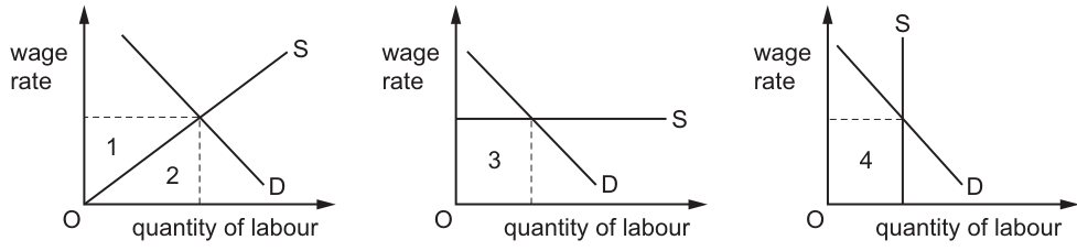
Which two areas represent economic rent?
Options
A 1 and 3
B 1 and 4
C 2 and 3
D 2 and 4
Answer
Economic rent is the payment to labour in excess of transfer earnings (opportunity cost). On a labour market diagram, it is represented by the area above the supply curve and below the wage rate.
In Diagram 1, the upward-sloping supply curve represents transfer earnings. Area 1 lies above the supply curve and below the equilibrium wage, so it represents economic rent. Area 2 lies below the supply curve and represents transfer earnings.
In Diagram 2, the horizontal supply curve indicates perfectly elastic supply, meaning workers can move to alternative jobs at the same wage. Consequently, there is no economic rent; all earnings equal transfer earnings. Area 3 represents total earnings, which are entirely transfer earnings.
In Diagram 3, the vertical supply curve indicates perfectly inelastic supply (a fixed quantity of labour). Area 4 represents the rectangle below the equilibrium wage and above the horizontal axis. Because the supply of labour is fixed and cannot respond to wage changes, this area represents economic rent.
Therefore, the two areas representing economic rent are 1 and 4.
Answer
B
B
Background Concept
Economic rent is the payment made to a factor of production that exceeds the minimum amount required to keep that factor in its current use. For labour, this means the wage paid above what workers could earn in their next best alternative employment—their transfer earnings. Transfer earnings represent the opportunity cost of supplying labour and are shown by the area under the labour supply curve up to the quantity employed. Economic rent is therefore the area between the supply curve and the wage rate, up to the quantity of labour employed. The size of economic rent depends on the elasticity of labour supply: it is zero when supply is perfectly elastic, positive when supply is upward-sloping or vertical, and equals total earnings when supply is perfectly inelastic.
Understanding the Question
The question presents three labour market diagrams (Fig. 14.1) showing different supply curve shapes and asks which two numbered areas represent economic rent. Diagram 1 shows an upward-sloping supply curve, Diagram 2 shows a horizontal (perfectly elastic) supply curve, and Diagram 3 shows a vertical (perfectly inelastic) supply curve. The candidate must identify which shaded areas correspond to economic rent (payment above transfer earnings) rather than transfer earnings themselves. The command word is implicit identification, requiring application of the definition of economic rent to each diagram.
Approach
To solve this, apply the definition: economic rent is the area above the supply curve and below the wage rate. Analyse each diagram in turn:
- Diagram 1 (upward-sloping supply): The supply curve slopes upward, indicating that higher wages are needed to attract more labour. Area 1 is above the supply curve and below the wage—this is economic rent. Area 2 is below the supply curve—this is transfer earnings.
- Diagram 2 (horizontal supply): A horizontal supply curve means workers can supply any quantity at that wage, typically because they can move freely to identical jobs. There is no economic rent because workers can earn the same wage elsewhere. Area 3 is below the supply curve and represents total earnings, which equal transfer earnings.
- Diagram 3 (vertical supply): A vertical supply curve means the quantity of labour is fixed regardless of the wage (perfectly inelastic supply). Area 4 is the rectangle below the equilibrium wage and above the horizontal axis. Because the quantity cannot increase even if the wage rises, the entire payment (or the area above the supply curve) constitutes economic rent.
Step-by-Step Reasoning
Diagram 1 Analysis:
The supply curve slopes upward from the origin, reflecting that as the wage rate rises, more workers are willing to supply their labour because higher wages are needed to overcome the opportunity cost of leisure or alternative employment. The equilibrium wage is determined where demand equals supply. Area 1 is the triangular area between the equilibrium wage line and the supply curve, up to the equilibrium quantity. This area represents the excess of actual earnings over transfer earnings—economic rent. Area 2 is the triangular area below the supply curve and above the horizontal axis, representing the transfer earnings (the minimum total payment required to induce workers to supply that quantity of labour).
Diagram 2 Analysis:
The supply curve is horizontal, indicating perfectly elastic supply. This means that at the going wage rate, workers are willing to supply any quantity of labour, but if the wage fell even slightly, they would supply zero labour because they could immediately move to other jobs paying the same rate. Because workers can earn the same wage in alternative employment, there is no economic rent. The entire earnings (Area 3, the rectangle between the wage and the horizontal axis) represent transfer earnings only.
Diagram 3 Analysis:
The supply curve is vertical, indicating perfectly inelastic supply. This means the quantity of labour is fixed—perhaps due to unique skills, professional licensing, or physical constraints—and does not change regardless of the wage rate. The demand curve determines the equilibrium wage. Area 4 is the rectangular area below the equilibrium wage and above the horizontal axis, up to the fixed quantity. Because the supply of labour is fixed and cannot be increased by raising the wage, the payment to these workers exceeds their transfer earnings (which are minimal or zero if the supply curve is drawn from the axis). Thus, Area 4 represents economic rent.
Conclusion: Areas 1 and 4 represent economic rent, making option B correct.
Key Takeaways
- Economic rent is the area above the supply curve and below the wage rate.
- Transfer earnings are the area under the supply curve.
- With upward-sloping supply, both economic rent and transfer earnings exist.
- With perfectly elastic (horizontal) supply, there is no economic rent.
- With perfectly inelastic (vertical) supply, all or most of the earnings are economic rent because the quantity is fixed.
Common Mistakes
- Confusing economic rent with transfer earnings: Students often identify Area 2 (transfer earnings in Diagram 1) or Area 3 (transfer earnings in Diagram 2) as economic rent.
- Assuming Area 3 is economic rent because it is a rectangle: In Diagram 2, the horizontal supply curve means workers face no excess payment, so Area 3 is purely transfer earnings.
- Misinterpreting Diagram 3: Students may think a vertical supply curve means no economic rent, but it actually means the fixed quantity generates economic rent because supply cannot respond to wage changes.
Things to Be Careful About
- Always locate the supply curve correctly: economic rent is strictly the area between the wage line and the supply curve, not the total area under the wage.
- Check the elasticity of supply: horizontal supply means zero economic rent; vertical supply means maximum economic rent.
- In Diagram 1, ensure you do not confuse the triangle above the supply curve (rent) with the triangle below it (transfer earnings).
- Remember that the question asks for TWO areas; verify that both selected areas fit the definition before choosing the option.
In an economy with no government sector or foreign trade, the marginal propensity to consume is 0.6.
If the equilibrium level of national income is $10 000 million and the full employment level of national income is $15 000 million, by how much would investment have to increase to achieve full employment?
Options
A $1666 million
B $2000 million
C $3012 million
D $5000 million
Working
Multiplier (k) = 1 / (1 - MPC) = 1 / (1 - 0.6) = 1 / 0.4 = 2.5
Output gap = full employment income - equilibrium income = $15 000 million - $10 000 million = $5 000 million
Required increase in investment = output gap / multiplier = $5 000 million / 2.5 = $2 000 million
Answer
B
B
Background Concept
This question tests the multiplier effect in a simple closed economy with no government and no foreign trade. The multiplier (k) shows the relationship between an initial change in autonomous expenditure (such as investment) and the resulting change in national income. In this simplified model, the only withdrawal from the circular flow is saving, so the multiplier formula is:
k = 1 / (1 - MPC) = 1 / MPS
where MPC is the marginal propensity to consume and MPS is the marginal propensity to save (MPS = 1 - MPC).
The multiplier works because one person's spending becomes another person's income, which is then partly spent again, creating a chain of additional rounds of spending. The size of the multiplier depends on how much of each additional unit of income is spent (the MPC) rather than saved.
Understanding the Question
The question describes an economy with:
- No government sector (no taxes, no government spending)
- No foreign trade (no exports or imports)
- MPC = 0.6
- Current equilibrium national income = $10 000 million
- Full employment national income = $15 000 million
It asks: by how much must investment increase to close the output gap and achieve full employment? This is a classic application of the multiplier: the change in income equals the multiplier times the change in autonomous spending.
Approach
- Calculate the multiplier using the given MPC.
- Calculate the size of the output gap (the difference between full employment income and current equilibrium income).
- Divide the output gap by the multiplier to find the required increase in investment.
Step-by-Step Reasoning
Step 1: Calculate the multiplier
MPC = 0.6, so MPS = 1 - 0.6 = 0.4
k = 1 / MPS = 1 / 0.4 = 2.5
This means that every $1 increase in autonomous spending (investment) will eventually increase national income by $2.50.
Step 2: Calculate the output gap
Output gap = Full employment income - Current equilibrium income
= $15 000 million - $10 000 million
= $5 000 million
This is the amount by which national income needs to rise.
Step 3: Calculate the required increase in investment
Since ΔY = k × ΔI, we rearrange to find ΔI = ΔY / k
ΔI = $5 000 million / 2.5 = $2 000 million
So investment must increase by $2 000 million. The multiplier of 2.5 will then generate a total increase in income of 2.5 × $2 000 million = $5 000 million, exactly closing the gap.
Checking the options:
- A: $1666 million would give ΔY = 2.5 × $1666m = $4165m, too small.
- B: $2000 million gives ΔY = 2.5 × $2000m = $5000m, correct.
- C: $3012 million gives ΔY = 2.5 × $3012m = $7530m, too large.
- D: $5000 million gives ΔY = 2.5 × $5000m = $12 500m, far too large.
Key Takeaways
- The multiplier formula in a closed economy with no government is k = 1 / (1 - MPC) = 1 / MPS.
- The output gap is the difference between full employment income and current equilibrium income.
- The required change in autonomous spending equals the output gap divided by the multiplier.
- Always check that the units are consistent (here, millions of dollars).
Common Mistakes
- Using the wrong multiplier formula: Some students might use k = 1 / MPC (which is incorrect) and get 1.67, leading to a wrong answer.
- Multiplying instead of dividing: A student might multiply the output gap by the multiplier ($5000m × 2.5 = $12 500m) and pick option D.
- Confusing the output gap: Some might think the gap is $15 000m - $10 000m = $5 000m but then forget to divide by the multiplier.
- Ignoring the multiplier entirely: A student might think investment must increase by the full $5 000m (option D), missing the multiplier effect entirely.
Things to Be Careful About
- The question specifies "no government sector or foreign trade" — this simplifies the multiplier to 1/(1-MPC). If there were taxes or imports, the formula would include the marginal propensity to tax (MPT) and the marginal propensity to import (MPM).
- The multiplier is 2.5, not 0.4. Remember that the multiplier is greater than 1 when MPC > 0.
- Units: all figures are in millions of dollars, so the answer is also in millions of dollars.
- The question asks for the increase in investment, not the new level of investment. The answer is the change, not the absolute amount.
What is a definition of hysteresis unemployment?
Options
A people who become temporarily unemployed because it takes a short period of time to find a job after they leave school
B people who become unemployed when there is a recession but who will find employment as the economy comes out of recession
C people who become unemployed for a long period of time due to a loss of job skills and work experience while unemployed
D people who become unemployed when established firms close and new firms are created as technology advances
Answer
Hysteresis unemployment occurs when a period of high unemployment permanently damages the employability of the long-term unemployed, so that even when aggregate demand recovers they remain out of work. The key feature is a loss of job skills and work experience while unemployed, which makes it structurally difficult for these workers to re-enter employment.
Answer
C
C
Background Concept
Hysteresis in economics refers to the idea that the past state of the economy (especially a deep or prolonged recession) can permanently alter its future path. In the labour market, hysteresis unemployment means that a temporary shock (e.g. a recession) can cause a permanent increase in the natural rate of unemployment. The mechanism is that workers who are unemployed for a long time lose their skills, become detached from the labour force, and may face stigma from employers, making it very difficult for them to find a job even when the economy recovers. This contrasts with cyclical unemployment, which is expected to reverse as the economy improves.
Understanding the Question
This is a straightforward multiple-choice question asking for the correct definition of "hysteresis unemployment". The four options each describe a different type of unemployment. The task is to identify which one matches the specific concept of hysteresis. The question tests knowledge of the precise meaning of this term, which is a key concept in the topic of unemployment.
Approach
Read each option carefully and compare it to the textbook definition of hysteresis unemployment. The defining characteristic is that the unemployment becomes persistent because the workers themselves become less employable over time. Eliminate options that describe other types of unemployment (frictional, cyclical, structural) and select the one that captures the loss of skills and long-term duration.
Step-by-Step Reasoning
- Option A describes frictional unemployment: people temporarily between jobs or entering the labour force. This is short-term and not associated with a loss of skills.
- Option B describes cyclical (or demand-deficient) unemployment: people lose jobs in a recession but are expected to find work again when the economy recovers. This is temporary and reversible, not permanent.
- Option C describes exactly the hysteresis mechanism: long-term unemployment leads to a deterioration of human capital (skills and experience), making it hard to re-enter employment even after the economy improves. This matches the definition.
- Option D describes structural unemployment caused by technological change: jobs disappear in declining industries and new jobs appear in growing industries, but workers may not have the right skills. While this can lead to long-term unemployment, the key feature of hysteresis is the self-reinforcing loss of skills due to the period of unemployment itself, not just a mismatch of skills. Option D is closer to standard structural unemployment.
Therefore, Option C is the correct answer.
Key Takeaways
- Hysteresis unemployment is a type of long-term unemployment where the experience of being unemployed itself reduces a worker's future employability.
- It is distinct from frictional, cyclical, and standard structural unemployment.
- The concept is important for understanding why unemployment can remain high even after the economy recovers from a recession.
Common Mistakes
- Confusing hysteresis with cyclical unemployment (Option B). The key difference is that cyclical unemployment is expected to reverse automatically with recovery, while hysteresis implies a permanent scar.
- Confusing hysteresis with structural unemployment caused by technological change (Option D). While both can lead to long-term unemployment, hysteresis specifically emphasises the loss of skills during unemployment, not just a mismatch of skills from the start.
Things to Be Careful About
- Read the precise wording of each option. The phrase "loss of job skills and work experience while unemployed" is the hallmark of hysteresis.
- Remember that hysteresis is about the persistence of unemployment beyond its initial cause.
An economy has a positive output gap.
What is happening to economic growth and the general price level?
Options
| economic growth | general price level | |
|---|---|---|
| A | above trend growth rate | falling |
| B | above trend growth rate | rising |
| C | below trend growth rate | falling |
| D | below trend growth rate | rising |
Answer
A positive output gap means actual GDP exceeds potential GDP. This occurs when the economy is growing above its trend rate, typically in the boom phase of the business cycle. As the economy operates beyond full capacity, demand-pull inflationary pressure causes the general price level to rise. Therefore, economic growth is above the trend growth rate and the general price level is rising.
Answer
B
B
Background Concept
An output gap is the difference between actual GDP and potential GDP (the maximum sustainable level of output an economy can produce when all resources are fully employed). A positive output gap occurs when actual GDP is greater than potential GDP, meaning the economy is producing beyond its sustainable capacity. This typically happens during the boom phase of the business cycle, when demand is very high and firms operate at above-normal capacity, often using overtime labour and older machinery. A positive output gap is associated with above-trend economic growth and upward pressure on the general price level (inflation). Conversely, a negative output gap (actual GDP below potential) occurs during a recession or slump, with below-trend growth and downward pressure on prices (disinflation or deflation).
Understanding the Question
This multiple-choice question asks: if an economy has a positive output gap, what is happening to (1) economic growth and (2) the general price level? The answer requires understanding that a positive output gap is not a static condition but arises from a phase of rapid expansion. The question tests the link between the output gap, the business cycle, and inflation. The four options combine two possibilities for growth (above or below trend) and two for the price level (rising or falling).
Approach
- Recall the definition of a positive output gap: actual output exceeds potential output.
- Recognise that this situation occurs when the economy is growing faster than its long-run trend rate — i.e., above-trend growth.
- Understand that when output exceeds potential, the economy is at or beyond full capacity. This creates demand-pull inflation as aggregate demand outstrips aggregate supply, so the general price level rises.
- Eliminate the options that contradict either of these two implications.
Step-by-Step Reasoning
-
Step 1: What does a positive output gap imply about economic growth?
A positive output gap means actual GDP is above potential GDP. For actual GDP to be above potential, the economy must have been growing at a rate faster than the growth rate of potential output (the trend growth rate). Therefore, economic growth is above the trend growth rate. This eliminates options C and D, which state "below trend growth rate". -
Step 2: What does a positive output gap imply about the general price level?
When the economy operates above its sustainable capacity, resources are scarce, and firms face rising costs. More importantly, aggregate demand is very strong relative to aggregate supply, creating demand-pull inflation. The general price level rises. This eliminates option A, which says "falling". -
Step 3: Select the correct option.
Only option B combines "above trend growth rate" with "rising" price level, which matches the implications of a positive output gap.
Key Takeaways
- A positive output gap = actual > potential = above-trend growth + rising prices (inflation).
- A negative output gap = actual < potential = below-trend growth + falling or stable prices (disinflation/deflation).
- The output gap is a key indicator of the business cycle phase and inflationary pressure.
Common Mistakes
- Confusing a positive output gap with a negative one: some students think a positive gap means the economy is doing well and prices might be stable, but the key is that it is unsustainable and inflationary.
- Thinking that a positive output gap means growth is "positive" (i.e., increasing) rather than "above trend". The question specifically asks about the growth rate relative to trend, not the sign of growth.
- Forgetting that a positive output gap is associated with rising prices (inflation), not falling prices.
Things to Be Careful About
- Distinguish between the level of output (actual vs potential) and the growth rate (above or below trend). A positive output gap implies the growth rate has been above trend to get there, but the gap itself is a level comparison.
- Remember that the general price level rises during a boom due to demand-pull inflation, not cost-push inflation (though both can occur). The question focuses on the demand-side pressure from the output gap.
What is a factor affecting the occupational mobility of labour?
Options
A education and training
B immigration controls
C price of housing
D transport infrastructure
Answer
Occupational mobility of labour refers to the ease with which workers can move between different occupations. The most direct factor affecting this is education and training, because acquiring new skills or qualifications enables a worker to enter a different occupation. Immigration controls affect the supply of labour from abroad, the price of housing and transport infrastructure affect geographical mobility (the ability to move between locations), not occupational mobility.
Answer
A
A
Background Concept
Occupational mobility of labour is a key concept in labour economics. It measures how easily workers can switch from one job or profession to another. This is distinct from geographical mobility, which measures how easily workers can move between different locations or regions. Factors that increase occupational mobility include transferable skills, general education, vocational training, and professional qualifications. Factors that reduce it include strict licensing requirements, strong trade union demarcation rules, and the specificity of human capital (skills that are only useful in one narrow field).
Understanding the Question
This is a straightforward multiple-choice question testing the distinction between the two types of labour mobility. The question asks for the factor that affects occupational mobility specifically. The four options are plausible distractors, but only one directly relates to the ability to change occupation.
Approach
Recall the definition of occupational mobility and identify which of the four options directly influences a worker's ability to move between occupations. Eliminate options that affect geographical mobility or the overall supply of labour.
Step-by-Step Reasoning
-
Option A: education and training – Education and training directly equip workers with the knowledge and skills needed for different occupations. A worker with a broad education or specific vocational training can more easily move into a new field. This is the classic textbook factor for occupational mobility.
-
Option B: immigration controls – Immigration controls affect the number of foreign workers entering a country. This influences the overall supply of labour in the economy, but it does not affect the ability of existing workers to change occupations. It is a factor affecting the size of the labour force, not its mobility between occupations.
-
Option C: price of housing – The price of housing affects where workers can afford to live. High housing costs in one area may prevent workers from moving there, but this is a factor affecting geographical mobility (moving between locations), not occupational mobility (moving between jobs).
-
Option D: transport infrastructure – Good transport infrastructure (roads, railways, public transport) makes it easier for workers to commute to different workplaces. This also affects geographical mobility, not occupational mobility.
Therefore, only education and training directly affect the ability to change occupation.
Key Takeaways
- Occupational mobility = ability to change job/profession.
- Geographical mobility = ability to change location.
- Education and training are the primary determinants of occupational mobility.
- Housing costs and transport affect geographical mobility.
- Immigration controls affect labour supply, not mobility.
Common Mistakes
- Confusing occupational mobility with geographical mobility. Many students pick housing or transport because they think of moving for a job, but that is about location, not occupation.
- Thinking that immigration controls affect mobility because they change the pool of workers. They affect the number of workers, not the ease of switching between jobs.
Things to Be Careful About
- Read the question carefully: it asks for a factor affecting occupational mobility, not labour mobility in general.
- Remember that the same factor can affect both types of mobility (e.g., training can also help a worker move to a new area if the skill is in demand there), but the question asks for the factor that is primarily associated with occupational mobility.
A country’s government decides to set artificially low interest rates.
What describes a negative consequence to this country of this policy?
Options
A a higher rate of consumer price inflation
B a rapid growth in gross domestic product
C an increase in investment by manufacturers and real estate developers
D a reduction in borrowing by consumers
Working
An artificially low interest rate means the central bank sets the rate below the market-clearing level. This makes borrowing cheaper, so consumers and firms borrow more. The increased spending raises aggregate demand (AD). If the economy is at or near full capacity, the rise in AD leads to demand-pull inflation.
Answer
A
A
Background Concept
The rate of interest is the price of credit — the cost of borrowing and the reward for saving. In a market economy, it is determined by the demand for and supply of loanable funds. A government (or central bank) can set an artificial (below-equilibrium) rate as part of an expansionary monetary policy. The key relationship here is that lower interest rates stimulate borrowing and spending, which shifts AD rightward. This, in turn, can create demand-pull inflation if the economy's supply side cannot fully respond.
Understanding the Question
The question asks specifically for a negative consequence of setting artificially low interest rates. The four options present various possible outcomes. Some (such as rapid GDP growth or increased investment) may appear positive, while others (such as higher inflation) are negative. The question tests your ability to trace the logical chain: low rates -> borrowing/spending -> AD -> inflation, and to recognise that even intended policy outcomes can have harmful side effects.
Approach
Start with the policy: artificially low interest rates (below equilibrium). Identify the immediate effect on borrowing and spending. Trace this through to aggregate demand, then to the price level. The negative consequence is inflation. Against this, check each option: A fits the chain. B and C describe positive outcomes (growth, investment), which are not 'negative consequences'. D (reduction in borrowing) is the opposite of what low rates cause. Therefore only A is correct.
Step-by-Step Reasoning
- Policy action: The government sets interest rates artificially low (i.e., below the level that would clear the loanable funds market).
- Immediate micro effect: The cost of borrowing falls. Consumers take on more loans for cars, houses, and credit card purchases. Firms borrow more for investment.
- Aggregate demand effect: This increased consumption and investment expenditure shifts the aggregate demand curve to the right.
- Impact on price level: If the economy is operating at or near full employment (i.e., on the Keynesian vertical or steep part of AS), the extra AD will mostly raise the price level rather than output. This is demand-pull inflation.
- Negative consequence: Higher consumer price inflation reduces the purchasing power of money, erodes real incomes, and may destabilise expectations. This is clearly a negative outcome.
Now evaluate the options:
- A: A higher rate of consumer price inflation. This is exactly the chain we just traced. Correct.
- B: A rapid growth in GDP. While this may occur, the question asks for a negative consequence. Growth is generally positive, so this is not a negative consequence. (Also, if the economy is at full capacity, growth may be limited anyway.)
- C: An increase in investment. Again, increased investment is generally positive (it raises future productive capacity). Not a negative consequence.
- D: A reduction in borrowing. This is the opposite of what happens — low rates encourage more borrowing, not less. Incorrect.
Key Takeaways
- Expansionary monetary policy (low interest rates) can boost AD but carries the risk of demand-pull inflation.
- When a question asks for a negative consequence, you must distinguish between intended policy outcomes (which may be positive) and the harmful side effects.
- Tracing a full chain of causation (policy -> borrowing -> spending -> AD -> price level) is essential for answering such questions correctly.
Common Mistakes
- Selecting a positive outcome: Some students see 'rapid GDP growth' as a consequence of low rates and assume it is negative because they think 'any outcome of a bad policy is negative'. But the question asks for the negative consequence, not for any consequence that could be listed.
- Confusing the sign of the effect: Students sometimes think low rates reduce borrowing (due to confusion with high rates). Low rates unambiguously make borrowing cheaper, so borrowing rises.
- Failing to link to inflation: Not noticing that increased AD in a near-full-capacity economy raises prices is a common omission.
Things to Be Careful About
- Read the wording carefully: 'negative consequence' is different from 'consequence' generally. Among the options, only one is unambiguously harmful.
- Remember that in the short run, low rates may boost output, but the question does not ask about short-run versus long-run trade-offs. It simply asks for the negative outcome, which is inflation.
- Keep your reasoning linear: cause -> immediate effect -> AD -> inflation. Don't get sidetracked by other possible effects (like currency depreciation, capital flows, etc.) unless relevant to the options.
According to the quantity theory of money, which combination would result in the general level of prices remaining unchanged?
Options
| money supply | total number of transactions | velocity of circulation | |
|---|---|---|---|
| A | remains unchanged | remains unchanged | rises by 3% |
| B | rises by 3% | remains unchanged | rises by 3% |
| C | rises by 3% | rises by 3% | remains unchanged |
| D | rises by 3% | rises by 3% | rises by 3% |
Working
The quantity theory of money states: MV = PT, where M = money supply, V = velocity of circulation, P = general price level, T = total number of transactions. For P to remain unchanged, the percentage change in MV must equal the percentage change in T.
Option C: M rises by 3%, T rises by 3%, V unchanged. Then MV rises by 3% and T rises by 3%, so P is unchanged.
All other options cause P to rise because the percentage change in MV exceeds the percentage change in T (A, B, D) or MV rises while T does not (A, B).
Answer
C
C
Background Concept
The quantity theory of money is a classical macroeconomic theory that describes the relationship between the money supply, the price level, and real output. It is often summarised by the equation of exchange: MV = PT (or MV = PQ, where Q is real output). Here:
- M = nominal money supply
- V = velocity of circulation (the average number of times a unit of currency is used to purchase goods and services in a given period)
- P = general price level
- T = total number of transactions (real volume of transactions)
The equation is an identity: it must hold by definition. In its simplest form, classical economists assumed that V and T are constant in the short run (V depends on institutional factors, T is at full employment output). Then a change in M leads proportionally to a change in P. However, this question relaxes the constancy assumption and asks: under what changes in M, V, and T does P remain unchanged?
Understanding the Question
We are given three variables: money supply (M), total number of transactions (T), and velocity of circulation (V). The general level of prices (P) is to remain unchanged. The question asks which combination of percentage changes in these variables leaves P unchanged, according to the quantity theory. Because the equation is proportional, we can think in terms of percentage changes: %Δ(MV) = %Δ(PT). If P is constant, %Δ(PT) = %ΔT (since %ΔP=0). Therefore, for P constant, %ΔM + %ΔV (approximately) must equal %ΔT. Actually exact for small changes: the product MV changes by (1+%ΔM)(1+%ΔV)-1, but the simple addition works for small percentages. For the given 3% changes, it's accurate enough.
Key: The condition for P unchanged is that the percentage change in (M×V) equals the percentage change in T.
Approach
We will test each option by computing whether %Δ(MV) equals %ΔT. For small changes, %Δ(MV) ≈ %ΔM + %ΔV. We'll check option C as the candidate, and also verify why the others fail.
Note: Option A: M unchanged, V rises 3% → MV rises by about 3%; T unchanged → P rises 3%. Option B: M rises 3%, V rises 3% → MV rises by about 6%; T unchanged → P rises. Option D: M rises 3%, V rises 3%, T rises 3% → MV rises by about 6%; T rises 3% → P rises by about 3%. Only option C: M and T both rise 3% and V unchanged → MV rises 3% and T rises 3% → P unchanged.
Step-by-Step Reasoning
- Write the quantity equation: MV = PT.
- If P is unchanged, then the right-hand side is simply T times a constant P, so the percentage change in PT equals percentage change in T.
- For the left-hand side, the percentage change in the product MV is approximately the sum of the percentage changes in M and V (since %Δ(MV) = (1+%ΔM)(1+%ΔV)-1 = %ΔM + %ΔV + (%ΔM)(%ΔV). For 3% changes, the cross term is 0.0009, negligible.
- Check each option:
- A: M unchanged (+0%), V +3% → MV increases ~3%. T unchanged (+0%). Since %ΔMV > %ΔT, P must increase (by ~3%). So P rises.
- B: M +3%, V +3% → MV increases ~6%. T unchanged → P rises (~6%).
- C: M +3%, V unchanged (+0%) → MV increases ~3%. T +3% → %ΔMV = %ΔT → P unchanged.
- D: M +3%, V +3% → MV increases ~6%. T +3% → %ΔMV (6%) > %ΔT (3%) → P rises (~3%).
- Only option C leaves P unchanged.
Note: The question assumes the equation holds and does not consider lags or other complications. It's a simple proportional test.
Key Takeaways
- The quantity equation MV = PT is an identity; it can be used to find how changes in money supply, velocity, and real transactions affect the price level.
- For the price level to remain constant, the proportional change in MV must equal the proportional change in T (real output/transactions).
- This is a core building block of monetarist theory: in the long run with V and T stable, changes in M lead to proportional changes in P.
Common Mistakes
- Forgetting that V can change: many students assume V is constant, leading them to think only M matters. Here V changes in three options.
- Confusing T with real output: T is the volume of transactions, which may be thought of as real GDP or total spending volume. The question uses "total number of transactions."
- Miscalculating the combined effect: for option D, some may think all three rising 3% leaves P unchanged, but actually the product MV rises more than T.
- Using additive arithmetic incorrectly: %Δ(MV) ≠ %ΔM + %ΔV in exact terms, but for small changes the approximation is fine. The exact calculation confirms the same result.
Things to Be Careful About
- Identify which variable is on which side: P and T are on the same side (PT). So for P constant, changes in T must be matched by changes in MV.
- Watch the direction: if MV rises more than T, P rises; if less, P falls.
- This question does not involve real output or the distinction between nominal and real GDP, but in more advanced contexts T is replaced by real output Q.
- The question is from a multiple-choice paper (Paper 1/3), so it tests quick reasoning. In an essay, you might also discuss the assumptions of the quantity theory.
A government increases its inflation rate target from 3% to 5%.
What is a likely reason for this?
Options
A to increase economic sustainability
B to increase saving
C to reduce a balance of payments deficit
D to reduce unemployment
Answer
Raising the inflation rate target from 3% to 5% is likely intended to reduce unemployment. According to the traditional Phillips curve, there is a short-run inverse relationship between inflation and unemployment. A higher inflation target allows the government to pursue more expansionary monetary or fiscal policy, which increases aggregate demand, raises output, and reduces unemployment. The other options are not consistent with a higher inflation target: higher inflation typically reduces economic sustainability (A), discourages saving (B), and worsens a balance of payments deficit (C) by making exports less competitive and imports cheaper.
Answer
D
D
Background Concept
The Phillips curve illustrates the short-run trade-off between inflation and unemployment. In the traditional (original) Phillips curve, lower unemployment is associated with higher inflation, and vice versa. This relationship arises because when aggregate demand increases, firms raise prices and also hire more workers to meet higher demand, pushing down unemployment but causing inflation to rise. Governments may choose a point on this curve that balances their objectives. A higher inflation target signals a willingness to accept more inflation in exchange for lower unemployment.
Understanding the Question
The question asks for the likely reason a government would increase its inflation target from 3% to 5%. The four options present possible objectives: increasing economic sustainability, increasing saving, reducing a balance of payments deficit, or reducing unemployment. The correct answer is the one that is consistent with the economic logic of a higher inflation target. The Phillips curve trade-off is the key concept: a higher inflation target implies the government is prioritising lower unemployment over price stability.
Approach
Evaluate each option against the consequences of higher inflation:
- Option A: Higher inflation generally reduces sustainability (e.g., erodes purchasing power, creates uncertainty), so this is unlikely.
- Option B: Higher inflation reduces the real value of savings, discouraging saving, not increasing it.
- Option C: Higher inflation makes exports more expensive and imports cheaper, worsening the current account deficit, not reducing it.
- Option D: Higher inflation can be associated with lower unemployment via the Phillips curve, making this the plausible reason.
Step-by-Step Reasoning
-
Identify the economic relationship: The traditional Phillips curve shows an inverse relationship between inflation and unemployment in the short run. A government that raises its inflation target is effectively choosing a point on the curve with higher inflation and lower unemployment.
-
Evaluate Option D: If the government wants to reduce unemployment, it can use expansionary policies (e.g., lower interest rates, increased government spending) that boost aggregate demand. This increases output and employment but also raises the inflation rate. By raising the inflation target, the government signals it is willing to tolerate higher inflation to achieve lower unemployment. This is a standard policy trade-off.
-
Evaluate Option A: Higher inflation typically reduces economic sustainability because it erodes the real value of money, distorts price signals, and can lead to uncertainty that discourages investment. A higher inflation target would not be chosen to increase sustainability.
-
Evaluate Option B: Higher inflation reduces the real return on savings, so people may save less. A government wanting to increase saving would aim for lower, more stable inflation, not a higher target.
-
Evaluate Option C: Higher inflation makes a country's exports relatively more expensive and imports cheaper, worsening the trade balance (assuming Marshall-Lerner conditions hold). To reduce a balance of payments deficit, a government would typically aim for lower inflation or a depreciation of the currency, not a higher inflation target.
-
Conclusion: Only Option D is consistent with the economic logic of a higher inflation target.
Key Takeaways
- The Phillips curve is a fundamental model showing the short-run trade-off between inflation and unemployment.
- A higher inflation target is a policy choice that prioritises lower unemployment over price stability.
- Higher inflation generally has negative effects on saving, the balance of payments, and sustainability, so those are not reasons to raise the target.
Common Mistakes
- Confusing the short-run Phillips curve trade-off with the long-run vertical Phillips curve (which shows no trade-off). The question refers to the short-run relationship.
- Thinking higher inflation helps the balance of payments (it actually worsens it by making exports less competitive).
- Assuming higher inflation encourages saving (it discourages saving because the real value of savings falls).
Things to Be Careful About
- The question asks for the "likely reason" — it is about policy motivation, not a guaranteed outcome.
- The traditional Phillips curve is the relevant model here; the expectations-augmented version (which shows no long-run trade-off) is not needed for this simple scenario.
- Be precise: higher inflation reduces unemployment only in the short run, but the question does not specify the time horizon, so the short-run trade-off is the standard answer.
What would be a macroeconomic policy objective for a government in a developed economy?
Options
A to improve sustainability
B to provide public goods
C to reduce the power of trade unions
D to subsidise the electricity supply industry
Answer
A. Sustainability is a recognised macroeconomic policy objective for a developed economy, alongside growth, inflation, balance of payments, unemployment, and redistribution.
A
Background Concept
Macroeconomic policy objectives are broad goals that a government pursues to manage the overall economy. For a developed economy, these typically include: low inflation, low unemployment, sustainable economic growth, a stable balance of payments, and a more equitable distribution of income. Sustainability has become an increasingly important objective, referring to the long-term viability of growth without depleting resources or harming the environment. Microeconomic policies, in contrast, target specific sectors or markets, such as the provision of public goods or the regulation of industries.
Understanding the Question
The question asks which of the four options is a macroeconomic policy objective. The key is to distinguish between economy-wide objectives and sector-specific or microeconomic interventions. The correct answer must be a goal that applies to the entire economy, not a policy tool for a particular market or industry.
Approach
Evaluate each option by asking: Is this a goal that affects the whole economy, or is it a specific policy applied to a particular sector? Use the typical list of macroeconomic objectives as a reference. The correct answer will match one of those objectives.
Step-by-Step Reasoning
- Option A: to improve sustainability – Sustainability is indeed a macroeconomic policy objective. It concerns the long-term health of the economy and the environment, ensuring that growth does not undermine future capacity. This is an economy-wide goal, so it fits.
- Option B: to provide public goods – Providing public goods (e.g., defence, street lighting) is a microeconomic function of government, addressing market failure. It is not a macroeconomic objective per se; it is a specific policy to correct a particular market failure.
- Option C: to reduce the power of trade unions – This is a labour market policy, often microeconomic in nature, aimed at altering the balance of power in wage negotiations. It is not a standard macroeconomic objective.
- Option D: to subsidise the electricity supply industry – This is a sector-specific industrial policy (subsidy) targeting one industry. It is a microeconomic intervention, not a macroeconomic objective.
Thus, only Option A is a macroeconomic policy objective.
Key Takeaways
- Macroeconomic objectives are economy-wide and include growth, inflation, unemployment, balance of payments, sustainability, and redistribution.
- Microeconomic policies target specific sectors or market failures (e.g., public goods, subsidies, labour market interventions).
- The question tests the ability to differentiate between these categories.
Common Mistakes
- Confusing a policy tool (e.g., subsidy, regulation) with an objective. The objective is the goal, not the means to achieve it.
- Thinking that any government action is a macroeconomic objective. Many government actions are microeconomic.
- Overlooking sustainability as a modern macroeconomic objective; it is now widely accepted.
Things to Be Careful About
- Read the exact wording: “macroeconomic policy objective” – not “policy” or “microeconomic objective”.
- Remember that “sustainability” is explicitly listed in the syllabus as a macroeconomic objective.
- Do not confuse a specific policy (like subsidising electricity) with an overall objective.
An economy is at its natural rate of unemployment.
Under which circumstances will an increase in government spending aimed at reducing unemployment be most likely to conflict with a government’s objective of low inflation?
Options
A if inflationary expectations are unchanged
B if inflationary expectations fall
C if labour productivity increases
D if labour supply increases
Reasoning
The economy is at its natural rate of unemployment, meaning there is no involuntary cyclical unemployment. Any increase in government spending will boost aggregate demand, shifting the economy along the short-run Phillips curve. If inflationary expectations are unchanged (option A), workers and firms do not immediately adjust their wage demands upward. In the short run, unemployment can fall below the natural rate, but only at the cost of higher inflation. This creates a direct conflict with the low-inflation objective.
If inflationary expectations fall (option B), the short-run Phillips curve shifts left, making the trade-off more favourable — lower inflation for any given unemployment rate — so the conflict is reduced. If labour productivity increases (option C) or labour supply increases (option D), the natural rate itself may fall, allowing higher output and employment without inflationary pressure. These options reduce or eliminate the conflict.
Answer
A
A
Background Concept
The Phillips curve illustrates the relationship between inflation and unemployment. The traditional (short-run) Phillips curve shows an inverse relationship: lower unemployment comes at the cost of higher inflation. The expectations-augmented Phillips curve incorporates the role of inflationary expectations. In the long run, the Phillips curve is vertical at the natural rate of unemployment — the rate consistent with stable inflation. Any attempt to push unemployment below the natural rate through demand-side policies will, in the long run, only cause higher inflation, not lower unemployment, once expectations adjust.
Understanding the Question
The question states the economy is already at its natural rate of unemployment. The government increases spending to reduce unemployment further. The question asks: under which of the four given circumstances will this policy most likely conflict with the objective of low inflation? The key is to identify which condition makes the short-run trade-off between unemployment and inflation most unfavourable — i.e., where the reduction in unemployment comes with the largest increase in inflation.
Approach
Evaluate each option in turn, considering how it affects the position of the short-run Phillips curve and the natural rate. The conflict is greatest when the short-run Phillips curve is steepest or when the natural rate is unchanged, so that any reduction in unemployment below the natural rate requires a large rise in inflation. Options that shift the short-run Phillips curve favourably (leftward) or lower the natural rate reduce the conflict.
Step-by-Step Reasoning
-
Option A: inflationary expectations are unchanged. The economy is at the natural rate. An increase in government spending shifts AD right. Along the existing short-run Phillips curve, unemployment falls below the natural rate, and inflation rises. Because expectations are unchanged, workers do not immediately demand higher wages to compensate for the higher inflation, so the reduction in unemployment is real in the short run. However, the inflation that results is a direct conflict with the low-inflation objective. This is the classic short-run trade-off.
-
Option B: inflationary expectations fall. A fall in expectations shifts the short-run Phillips curve leftward. For any given unemployment rate, inflation is lower. If the government then increases spending, the resulting inflation is lower than it would have been with unchanged expectations. The conflict with the low-inflation objective is reduced, not increased.
-
Option C: labour productivity increases. Higher productivity means each worker produces more output. This shifts the long-run aggregate supply curve right, lowering the natural rate of unemployment (or at least allowing higher output without inflationary pressure). The economy can now sustain a lower unemployment rate without generating extra inflation. The conflict is reduced.
-
Option D: labour supply increases. A larger labour force, if matched by demand, can also lower the natural rate (or allow higher employment without wage pressure). Again, the conflict is reduced.
Therefore, the circumstance that makes the conflict most likely is unchanged inflationary expectations (A).
Key Takeaways
- The natural rate of unemployment is the rate at which inflation is stable. Any attempt to push unemployment below it through demand-side policies will, in the short run, cause higher inflation.
- The expectations-augmented Phillips curve shows that the short-run trade-off depends on inflationary expectations. Unchanged expectations mean the trade-off is fully present.
- Factors that lower the natural rate (productivity growth, increased labour supply) or shift the short-run Phillips curve favourably (falling expectations) reduce the policy conflict.
Common Mistakes
- Confusing the short-run and long-run Phillips curves. The question asks about the short-run conflict, not the long-run outcome.
- Thinking that any increase in government spending always causes inflation. The effect depends on where the economy is relative to the natural rate and on expectations.
- Selecting option C or D because they seem to help reduce unemployment — but the question asks which makes the conflict most likely, not which helps.
Things to Be Careful About
- The economy is already at the natural rate. This is crucial — there is no spare capacity to absorb the extra demand without inflation.
- The phrase 'most likely' means we are comparing the four options, not evaluating the policy in isolation.
- Understand that 'inflationary expectations' refer to what workers and firms expect future inflation to be, which influences wage-setting and price-setting behaviour.
An economy imports a large proportion of its raw materials. Its exchange rate depreciates.
What is the impact on the external and internal value of money?
Options
| external value of money | internal value of money | |
|---|---|---|
| A | rises | rises |
| B | rises | falls |
| C | falls | rises |
| D | falls | falls |
Answer
A depreciation of the exchange rate means that the domestic currency buys fewer units of foreign currency, so the external value of money falls. Since the economy imports a large proportion of its raw materials, the depreciation raises the domestic price of these imports, increasing firms' costs of production. This leads to cost-push inflation, reducing the purchasing power of money domestically, so the internal value of money also falls. Therefore both external and internal values fall.
Answer
D
D
Background Concept
The external value of money refers to the purchasing power of a currency in international markets, i.e., the exchange rate. A depreciation means the currency is worth less in terms of foreign currency. The internal value of money refers to its purchasing power within the domestic economy, which is inversely related to the price level. When the general price level rises (inflation), the internal value falls.
Understanding the Question
The question states that an economy imports a large proportion of its raw materials and its exchange rate depreciates. We are asked to determine the impact on both the external and internal value of money. The command word "What is the impact" requires identification of the direction of change for each. This is a multiple-choice question, so we must select the correct combination from the options.
Approach
First, consider the external value: a depreciation directly reduces the external value because the currency can now buy less foreign currency. Second, consider the internal value: the depreciation makes imported raw materials more expensive, raising production costs. Firms pass on these higher costs to consumers, leading to a higher price level (inflation), which reduces the internal value of money. Therefore both values fall.
Step-by-Step Reasoning
-
External value: The exchange rate is the price of domestic currency in terms of foreign currency. A depreciation means that more domestic currency is needed to buy a unit of foreign currency, so the domestic currency is worth less externally. Hence the external value falls.
-
Internal value: The internal value is the purchasing power of money within the economy, which is the inverse of the price level. When the price level rises, the internal value falls. The depreciation raises the domestic price of imported raw materials because the same quantity of foreign currency now costs more domestic currency. Since raw materials are inputs for production, firms face higher costs. To maintain profit margins, they raise the prices of final goods and services. This cost-push inflation increases the general price level, so the internal value of money falls.
-
Combined effect: Both external and internal values fall. This corresponds to option D.
Key Takeaways
- The external value of money is the exchange rate; depreciation reduces it.
- The internal value of money is the purchasing power; inflation reduces it.
- Depreciation can cause inflation if the economy relies heavily on imported inputs, leading to cost-push inflation.
- The relationship between external and internal value is not always one-to-one; it depends on the structure of the economy.
Common Mistakes
- Confusing external and internal value: some might think depreciation raises external value because exports become cheaper, but external value is about the currency's worth, not the price of exports.
- Ignoring the import dependence: without considering that raw materials are imported, one might think internal value is unaffected by depreciation.
- Selecting option B (external rises, internal falls) by mistakenly thinking depreciation strengthens the currency.
Things to Be Careful About
- Distinguish between nominal and real exchange rates; the question refers to nominal depreciation.
- Internal value is the inverse of the price level; a fall in internal value means inflation.
- The condition "imports a large proportion of its raw materials" is crucial; without it, the impact on internal value might be smaller or delayed.
- Ensure to answer both parts of the question: external and internal value.
A country’s government imposes a tariff on steel imports.
What is the likely impact of this tariff on this country’s economy?
Options
A It will make this country’s steel exports more price competitive.
B It will lead to productive inefficiency in this country’s steel industry.
C There will be an improvement in this country’s terms of trade.
D There will be a decrease in producer surplus for this country’s steel producers.
Reasoning
A tariff raises the domestic price of imported steel, allowing domestic steel producers to charge a higher price than the world price. This reduces the competitive pressure on domestic firms to minimise costs, leading to X-inefficiency and productive inefficiency (producing above the minimum point of the average cost curve).
Option A is incorrect: the tariff does not affect the price of the country's steel exports; it only affects imports.
Option C is incorrect: the terms of trade (export prices / import prices) may improve if import prices rise, but this is not the primary or certain impact; the question asks for the likely impact, and productive inefficiency is a direct consequence.
Option D is incorrect: the tariff raises the domestic price, increasing producer surplus for domestic steel producers, not decreasing it.
Answer
B
B
Background Concept
A tariff is a tax on imported goods. It raises the domestic price of the imported good above the world price. This protects domestic producers from foreign competition by making imports more expensive. The key economic effects of a tariff include:
- Higher domestic price: Consumers pay more for the good.
- Increased domestic production: Domestic firms expand output because they can now compete with the higher-priced imports.
- Reduced consumer surplus: Consumers lose because they pay more.
- Increased producer surplus: Domestic producers gain because they receive a higher price.
- Government revenue: The government collects tariff revenue.
- Deadweight loss: There is a net welfare loss to the economy due to inefficient domestic production and reduced consumption.
Productive efficiency occurs when a firm produces at the minimum point of its average cost curve. When protected from competition, firms have less incentive to minimise costs, leading to X-inefficiency and productive inefficiency.
Understanding the Question
This is a multiple-choice question asking for the likely impact of a tariff on the importing country's economy. The question does not specify the market structure of the domestic steel industry, but the standard analysis assumes a competitive market initially. The four options test understanding of:
- A: Whether a tariff improves export competitiveness (it does not; it only affects imports).
- B: Whether a tariff leads to productive inefficiency (yes, by reducing competitive pressure).
- C: Whether a tariff improves the terms of trade (possibly, but not the most direct or likely impact).
- D: Whether a tariff decreases producer surplus for domestic producers (it increases it).
The correct answer is B because the protective effect of a tariff reduces the incentive for domestic firms to be efficient, leading to productive inefficiency.
Approach
- Recall the standard effects of a tariff on domestic price, output, and efficiency.
- Evaluate each option against these effects.
- Identify the option that is a direct and likely consequence.
Step-by-Step Reasoning
Step 1: Understand the effect of a tariff on domestic price.
A tariff raises the domestic price of the imported good above the world price. Domestic producers can now sell at this higher price, which is above the world price. This reduces the competitive pressure from foreign firms.
Step 2: Analyse the impact on domestic efficiency.
In a competitive market without a tariff, domestic firms must produce at the lowest possible cost to survive. With a tariff, they can charge a higher price and still sell their output. This reduces the incentive to minimise costs, leading to X-inefficiency (the firm operates above its minimum average cost). This is productive inefficiency.
Step 3: Evaluate each option.
- Option A: The tariff does not affect the price of the country's exports. It only affects imports. Therefore, it does not make exports more price competitive. Incorrect.
- Option B: As explained, the tariff reduces competitive pressure, leading to productive inefficiency. This is a direct and likely impact. Correct.
- Option C: The terms of trade (export prices / import prices) may improve if import prices rise, but this is not certain (it depends on the size of the tariff and the response of export prices). Moreover, the question asks for the likely impact, and productive inefficiency is more direct and certain. Incorrect.
- Option D: The tariff raises the domestic price, so domestic producers receive a higher price for each unit sold. This increases producer surplus, not decreases it. Incorrect.
Step 4: Conclusion.
The correct answer is B.
Key Takeaways
- A tariff protects domestic industries from foreign competition, reducing the incentive for cost minimisation and leading to productive inefficiency.
- A tariff increases domestic producer surplus, not decreases it.
- A tariff does not directly affect export competitiveness.
- The terms of trade may improve, but this is not the most direct or certain impact.
Common Mistakes
- Confusing producer surplus with consumer surplus: Students may think a tariff hurts domestic producers, but it actually helps them by raising the price.
- Thinking a tariff improves export competitiveness: A tariff only affects imports; it does not make exports cheaper.
- Overlooking the efficiency effect: Students may focus on the terms of trade effect and miss the more direct impact on productive efficiency.
Things to Be Careful About
- Read the question carefully: it asks for the likely impact, not the only possible impact.
- Distinguish between the effects on domestic producers (higher price, higher surplus, less efficiency) and consumers (higher price, lower surplus).
- Remember that productive inefficiency arises from reduced competitive pressure, not from the tariff itself directly causing higher costs.
Which measurement is not included in the calculation of the Human Development Index?
Options
A average years of schooling
B Gross National Income per capita
C infant mortality rate
D life expectancy at birth
Answer
The Human Development Index (HDI) is a composite index that combines three dimensions: life expectancy at birth (health), years of schooling (education), and gross national income per capita (standard of living). Infant mortality rate is not a component of the HDI; it is a separate indicator of health outcomes. Therefore, the correct answer is C.
C
Background Concept
The Human Development Index (HDI) is a composite statistic used to rank countries by level of 'human development'. It is published by the United Nations Development Programme (UNDP) and is calculated from three equally weighted dimensions:
- Health: measured by life expectancy at birth.
- Education: measured by mean years of schooling for adults aged 25+ and expected years of schooling for children of school entering age.
- Standard of living: measured by Gross National Income (GNI) per capita adjusted for purchasing power parity (PPP).
Each dimension is normalised to a value between 0 and 1, and the geometric mean of the three indices gives the final HDI score.
Understanding the Question
This is a straightforward multiple-choice question that asks which of the four listed measurements is not used in calculating the HDI. The options are:
- A: average years of schooling (part of the education dimension)
- B: Gross National Income per capita (the income dimension)
- C: infant mortality rate (a separate health indicator)
- D: life expectancy at birth (the health dimension)
Only option C is not a direct component of the HDI.
Approach
Recall the three dimensions of the HDI and match each option to the dimension it belongs to. The option that does not fit any of the three dimensions is the correct answer.
Step-by-Step Reasoning
- List the three HDI dimensions: health, education, income.
- Option A (average years of schooling) is a core part of the education dimension. It is one of the two education indicators used.
- Option B (GNI per capita) is the income dimension indicator. GNI per capita (PPP) is used.
- Option D (life expectancy at birth) is the health dimension indicator. It reflects the overall health status of the population.
- Option C (infant mortality rate) is also a health indicator, but it is not one of the three HDI components. The HDI uses life expectancy, not infant mortality. Although infant mortality influences life expectancy, it is a separate measure and is not included in the HDI formula.
Therefore, the correct answer is C.
Key Takeaways
- The HDI comprises three dimensions: health (life expectancy), education (years of schooling), and income (GNI per capita).
- Other common development indicators, such as infant mortality rate, poverty rate, or inequality measures, are not directly part of the HDI.
- Knowing the exact components of the HDI is essential for questions about composite indicators.
Common Mistakes
- Confusing infant mortality rate with life expectancy: they are related but distinct. Infant mortality rate is a separate indicator, not part of the HDI.
- Thinking that any health-related indicator automatically belongs to the HDI. The HDI specifically uses life expectancy at birth.
Things to Be Careful About
- The HDI uses GNI per capita, not GDP per capita. The question uses GNI per capita, which is correct.
- The HDI has been updated over time; the current version uses gross national income per capita (PPP) and mean years of schooling. Ensure you use the most up-to-date definition.
- For multiple-choice questions, read each option carefully and match it to the defined components.
The diagram shows the impact of a revaluation of a country’s exchange rate on the current account of the balance of payments.
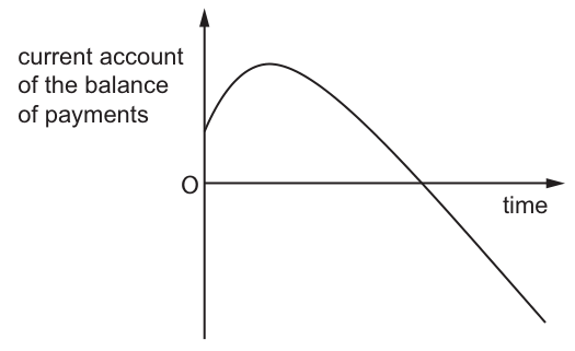
The table gives the price elasticity of demand for imports, PEDM, and the price elasticity of demand for exports, PEDX, in both the short run and the long run.
Which combination of short run and long run elasticities will give the shape shown in the diagram?
Options
| short run | long run | |||
|---|---|---|---|---|
| PEDM | PEDX | PEDM | PEDX | |
| A | 0.2 | 0.2 | 0.4 | 0.4 |
| B | 0.4 | 0.4 | 0.8 | 0.8 |
| C | 0.8 | 0.8 | 1.2 | 1.2 |
| D | 1.2 | 1.2 | 1.6 | 1.6 |
Working
The diagram shows the J-curve effect following an exchange rate revaluation: the current account initially rises (improves) to a peak, then falls (deteriorates) over time, eventually moving into deficit.
For a revaluation to cause an initial short-run improvement in the current account, the sum of the price elasticities of demand for imports (PEDM) and exports (PEDX) in the short run must be less than 1, so the price effect of the revaluation dominates the quantity effect. In the long run, elasticities are higher as consumers and firms adjust their behaviour; for the current account to deteriorate in the long run, the long-run sum of PEDM and PEDX must be greater than 1, so the quantity effect dominates.
Checking the options:
- Option A: Short-run sum = 0.2 + 0.2 = 0.4 <1; long-run sum = 0.4 + 0.4 = 0.8 <1. Long-run CA would continue to improve, which does not match the diagram.
- Option B: Short-run sum = 0.4 + 0.4 = 0.8 <1 (initial CA improvement); long-run sum = 0.8 + 0.8 = 1.6 >1 (long-run CA deterioration). This matches the diagram.
- Option C: Short-run sum = 0.8 + 0.8 = 1.6 >1, so CA would fall immediately with no initial peak. Incorrect.
- Option D: Short-run sum = 1.2 + 1.2 = 2.4 >1, so CA would fall immediately. Incorrect.
Answer
B
B
Background Concept
This question tests two linked exchange rate concepts: the J-curve effect and the Marshall-Lerner condition.
A revaluation is an upward adjustment of a country's currency value under a fixed or managed exchange rate system, making exports more expensive to foreign buyers and imports cheaper for domestic buyers. This affects the current account of the balance of payments, which records the value of exports minus the value of imports of goods and services.
The J-curve effect describes the time path of the current account following a change in the exchange rate. It arises because price elasticities of demand for imports and exports are lower in the short run than in the long run: consumers and firms take time to adjust their purchasing habits, find alternative suppliers or markets, and amend long-term contracts, so quantities demanded are relatively insensitive to price changes in the short run.
The Marshall-Lerner condition states that a depreciation of the currency will improve the current account in the long run only if the sum of the absolute values of the price elasticity of demand for exports (PEDX) and the price elasticity of demand for imports (PEDM) is greater than 1. For a revaluation, the opposite applies: if the sum is greater than 1, the current account will deteriorate in the long run, as the quantity effects of the price changes dominate the initial price effects.
Understanding the Question
The question provides a diagram of the current account over time after a revaluation, and a table of short-run and long-run PEDM and PEDX values for four options. The task is to identify which combination of elasticities produces the J-curve shape shown: an initial rise in the current account to a peak, followed by a fall that takes the current account into deficit (below the horizontal axis).
This shape is the reverse of the standard J-curve seen after a depreciation (where the current account first falls then rises). For a revaluation, the initial rise in the current account occurs because short-run trade elasticities are low, so the price effect of the revaluation dominates. The subsequent fall occurs because long-run elasticities are higher, so the quantity effect dominates. The key is that short-run elasticities are low (sum <1) and long-run elasticities are high enough that their sum is greater than 1.
Approach
To solve this, follow these steps:
- Interpret the diagram: confirm it shows an initial short-run improvement in the current account, followed by long-run deterioration. This means the price effect of the revaluation dominates in the short run, and the quantity effect dominates in the long run.
- Recall the Marshall-Lerner condition logic: for the price effect to dominate in the short run, the sum of short-run PEDM and PEDX must be less than 1. For the quantity effect to dominate in the long run (causing CA deterioration after a revaluation), the sum of long-run PEDM and PEDX must be greater than 1.
- Check each option against these two requirements, eliminating any that do not fit.
Step-by-Step Reasoning
First, analyse the effect of a revaluation on the current account:
- A revaluation raises the domestic currency value of exports (they are more expensive for foreigners) and lowers the domestic currency value of imports (they are cheaper for domestic buyers).
- The change in the value of exports equals (new export price * new export quantity) minus (old export price * old export quantity). The change in import value follows the same logic. The current account (CA) is export value minus import value.
In the short run: - PEDX and PEDM are low (inelastic, less than 1 in absolute value), because quantities adjust slowly. So the rise in export price leads to only a small fall in export quantity, so total export value rises. The fall in import price leads to only a small rise in import quantity, so total import value falls. Both effects improve the CA, so CA rises to a peak. This requires that the sum of |PEDX| and |PEDM| is less than 1: if the sum were greater than 1, the quantity effects would already be large enough to offset the price effects, and CA would fall immediately.
In the long run: - PEDX and PEDM are higher (more elastic, with a sum greater than 1 in absolute value), as consumers and firms have time to adjust. The large fall in export quantity (due to higher export prices) reduces total export value, and the large rise in import quantity (due to lower import prices) increases total import value. Both effects worsen the CA, so CA falls, eventually moving into deficit.
Now evaluate each option: - Option A: Short-run sum = 0.2 + 0.2 = 0.4 <1 (fits short run), but long-run sum = 0.4 + 0.4 = 0.8 <1. If long-run sum is less than 1, the price effect still dominates, so CA would continue to improve in the long run, not fall as shown. Eliminate A.
- Option B: Short-run sum = 0.4 + 0.4 = 0.8 <1 (fits short run: CA rises to peak). Long-run sum = 0.8 + 0.8 = 1.6 >1 (fits long run: CA falls into deficit). This matches the diagram exactly.
- Option C: Short-run sum = 0.8 + 0.8 = 1.6 >1. The quantity effect already dominates in the short run, so CA would fall immediately after revaluation, with no initial peak. Eliminate C.
- Option D: Short-run sum = 1.2 + 1.2 = 2.4 >1, same problem as C: no initial rise in CA. Eliminate D.
Thus, option B is the correct combination.
Key Takeaways
- The J-curve effect for a revaluation is the reverse of that for a depreciation: initial current account improvement, followed by long-run deterioration, if the Marshall-Lerner condition holds in the long run.
- The Marshall-Lerner condition depends on the sum of the absolute values of PEDX and PEDM: if the sum is greater than 1, the quantity effect of an exchange rate change dominates in the long run; if less than 1, the price effect dominates.
- Price elasticities of demand for trade are lower in the short run than in the long run, due to adjustment costs, contracts, and habit, which creates the J-curve shape.
Common Mistakes
- Confusing the J-curve for a revaluation with that for a depreciation: students often memorise the standard depreciation J-curve (initial CA deterioration, then improvement) and forget that a revaluation produces the opposite trajectory, leading them to eliminate the correct option.
- Misapplying the Marshall-Lerner condition: forgetting that for a revaluation, a sum of elasticities greater than 1 leads to long-run CA deterioration, not improvement.
- Ignoring the time dimension of elasticities: the question explicitly distinguishes short-run and long-run elasticities, so options where short-run elasticities are already high (sum >1) can be eliminated immediately, as they would not produce the initial peak in the CA.
Things to Be Careful About
- Always link the shape of the diagram to the time path of elasticities: the initial rise requires low short-run elasticities (sum <1), the subsequent fall requires higher long-run elasticities (sum >1).
- Remember that the Marshall-Lerner condition uses the sum of the absolute values of PEDX and PEDM, so ignore the negative signs of the elasticities when adding them.
- Check that the long-run outcome matches the diagram: the diagram shows CA falling into negative territory, so long-run sum of elasticities must be greater than 1, eliminating options where the long-run sum is less than 1.
What is not a function of the International Monetary Fund (IMF)?
Options
A to encourage exchange rate stability
B to provide financial assistance for a country with failed economic policies
C to provide funds for a water purifying plant in a developing country
D to provide loans for countries following a natural disaster
Answer
The IMF's core functions include promoting exchange rate stability, providing temporary financial assistance to countries with balance of payments difficulties (which can result from failed economic policies), and providing emergency loans after natural disasters. Funding specific infrastructure projects, such as a water purifying plant in a developing country, is the role of the World Bank, not the IMF. Therefore, option C is not a function of the IMF.
C
Background Concept
The International Monetary Fund (IMF) and the World Bank are two distinct international financial institutions created at the Bretton Woods Conference in 1944, but they have different purposes. The IMF's primary role is to ensure the stability of the international monetary system—the system of exchange rates and international payments that enables countries to transact with each other. It focuses on macroeconomic issues: exchange rate stability, balance of payments crises, and global financial stability. It provides short-to-medium-term loans to countries facing balance of payments problems, often with conditions (austerity measures, structural reforms) attached. The World Bank, on the other hand, is a development institution focused on reducing poverty and promoting long-term economic development. It provides long-term loans, grants, and technical assistance for specific projects in areas like infrastructure, education, health, and water supply. Knowing this distinction is key to answering the question.
Understanding the Question
The question asks which of the four listed activities is NOT a function of the IMF. This is a test of your knowledge of the specific roles of the IMF versus other international organisations, particularly the World Bank. The options present four plausible activities: encouraging exchange rate stability, providing financial assistance for failed policies, funding a specific infrastructure project, and providing loans after a natural disaster. You need to identify the one that falls outside the IMF's mandate.
Approach
- Recall the core functions of the IMF: surveillance of the global economy, providing financial assistance to countries with balance of payments problems, and offering technical assistance and training.
- Recall the core functions of the World Bank: providing loans and grants for specific development projects (infrastructure, health, education, etc.) in developing countries.
- Evaluate each option against these functions. Options A, B, and D align with the IMF's role. Option C aligns with the World Bank's role.
Step-by-Step Reasoning
- Option A: to encourage exchange rate stability. This is a core function of the IMF. It monitors the exchange rate policies of its member countries and provides a forum for cooperation on international monetary issues to prevent competitive devaluations and promote a stable system of exchange rates. This is a correct function.
- Option B: to provide financial assistance for a country with failed economic policies. When a country's economic policies lead to a balance of payments crisis (e.g., a large current account deficit, a currency crisis), the IMF provides loans to help the country stabilise its economy, rebuild reserves, and implement corrective policies. This is a classic IMF function. This is a correct function.
- Option C: to provide funds for a water purifying plant in a developing country. This is a specific, long-term infrastructure project. Funding such a project is the role of the World Bank (specifically, the International Bank for Reconstruction and Development or the International Development Association). The IMF does not fund specific projects; it provides general budget support to address macroeconomic imbalances. This is NOT a function of the IMF.
- Option D: to provide loans for countries following a natural disaster. The IMF has facilities like the Rapid Credit Facility (RCF) and the Rapid Financing Instrument (RFI) that provide rapid, low-conditionality financial assistance to countries facing urgent balance of payments needs, including those caused by natural disasters. This is a correct function.
Since options A, B, and D are all functions of the IMF, the only one that is not is option C.
Key Takeaways
- The IMF focuses on the stability of the international monetary system and provides short-to-medium-term loans for balance of payments support.
- The World Bank focuses on long-term economic development and provides loans and grants for specific projects.
- A common exam trick is to confuse the roles of the IMF and the World Bank. Remember: IMF = stability and crisis loans; World Bank = development projects.
Common Mistakes
- Confusing the IMF with the World Bank: This is the most common mistake. Students often think both institutions do the same thing. The key is to remember the IMF deals with macroeconomic crises and exchange rates, while the World Bank deals with long-term development projects.
- Overthinking the 'failed economic policies' option: Some students might think the IMF only helps with external shocks, not policy failures. However, the IMF's primary purpose is to help countries correct balance of payments problems, which are often the result of poor domestic policies.
Things to Be Careful About
- Read the question carefully: The question asks for what is NOT a function. It is easy to accidentally select an option that IS a function.
- Distinguish between 'balance of payments support' and 'project funding': The IMF provides general budget support to stabilise the economy. The World Bank provides funding for specific, tangible projects. This is the clearest distinction between the two institutions.
The diagram shows the effect of trade creation if a tariff is removed.
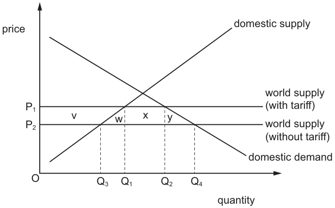
Which areas show the total net gain to the domestic economy?
Options
A v, w, x and y
B v, w and x only
C w and x only
D w and y only
Working
When the tariff is removed, the price falls from P1 to P2.
- Consumer surplus increases by the area between P1 and P2 up to Q4: v + w + x + y.
- Producer surplus decreases by the area between P1 and P2 up to Q1: v + w.
- Government tariff revenue (area x) is lost.
- The net gain to the domestic economy is the elimination of the deadweight welfare losses: the production distortion (w) and the consumption distortion (y). Areas v and x represent transfers (from producers and government to consumers), not net gains.
Answer
D
D
Background Concept
Trade creation occurs when a country removes a tariff (or reduces it) and switches from buying a good from a higher-cost domestic producer to a lower-cost foreign producer. This improves allocative efficiency because resources move from less efficient domestic production to more efficient foreign production, and consumers gain from the lower price.
In welfare analysis, the total surplus of the domestic economy is the sum of consumer surplus (CS), producer surplus (PS), and government revenue (GR). When a tariff is removed:
- CS increases because consumers pay a lower price and buy more.
- PS decreases because domestic producers receive a lower price and produce less.
- GR decreases (or falls to zero) because the tariff revenue is no longer collected.
The net welfare effect depends on whether the gains in CS exceed the losses in PS and GR. The net gain consists of the two deadweight loss triangles that are eliminated: the production efficiency gain (resources freed from inefficient domestic production) and the consumption efficiency gain (consumers valuing the additional units more than the world price).
Understanding the Question
The diagram shows a small country facing a horizontal world supply curve. With the tariff, the price is P1; without the tariff, the price is P2. The areas between these prices are labelled v, w, x, and y. The question asks which areas represent the total net gain to the domestic economy when the tariff is removed.
Key information from the diagram:
- At price P1 (with tariff): domestic supply is Q1, domestic demand is Q2.
- At price P2 (without tariff): domestic supply is Q3, domestic demand is Q4.
- Area v lies to the left of the domestic supply curve between P1 and P2.
- Area w is the triangle between the domestic supply curve and the vertical line at Q1.
- Area x is the rectangle between Q1 and Q2.
- Area y is the triangle between the vertical line at Q2 and the domestic demand curve.
The phrase "total net gain" is crucial. It does not mean the gain in consumer surplus, but the overall change in national welfare (CS + PS + GR). Transfers between groups are not net gains.
Approach
To find the net gain, calculate the change in each component of total surplus:
- Change in CS = + (v + w + x + y)
- Change in PS = - (v + w)
- Change in GR = - x
- Net gain = Change in CS + Change in PS + Change in GR
Alternatively, recognise that the net gain equals the deadweight loss triangles that are eliminated when the tariff is removed: the production distortion (w) and the consumption distortion (y).
Step-by-Step Reasoning
Step 1: Identify the initial position (with tariff)
The world price with tariff is P1. At this price, domestic producers supply Q1 and domestic consumers demand Q2. The government collects tariff revenue on the imports (Q2 - Q1), which is represented by area x.
Step 2: Identify the new position (without tariff)
The world price falls to P2. Domestic producers now supply only Q3 (where P2 intersects domestic supply), and domestic consumers demand Q4 (where P2 intersects domestic demand). Imports rise to (Q4 - Q3).
Step 3: Analyse the change in consumer surplus
Consumers benefit from the lower price and greater availability. Their surplus increases by the entire area between P1 and P2 up to the new quantity demanded Q4. This area comprises v + w + x + y.
Step 4: Analyse the change in producer surplus
Domestic producers lose because they receive a lower price and sell less. Their surplus decreases by the area between P1 and P2 up to the original quantity supplied Q1. This area comprises v + w.
Step 5: Analyse the change in government revenue
The government no longer collects the tariff, so it loses area x.
Step 6: Calculate the net gain
Net gain = Gain in CS - Loss in PS - Loss in GR
Net gain = (v + w + x + y) - (v + w) - x
Net gain = w + y
Area w represents the production efficiency gain: resources previously used in inefficient domestic production (between Q3 and Q1) are freed up for more productive uses elsewhere. Area y represents the consumption efficiency gain: consumers who value the good above the world price P2 but below the tariff-inclusive price P1 can now purchase it, creating value.
Areas v and x are transfers, not net gains. Area v is transferred from producers to consumers. Area x is transferred from the government to consumers (as lower prices). Neither creates new welfare; they merely redistribute existing welfare.
Key Takeaways
- Trade creation results in a net welfare gain equal to the sum of the production and consumption distortion triangles (w + y).
- When analysing tariff removal, always calculate the change in total surplus (CS + PS + GR), not just the change in consumer surplus.
- Transfers (such as the redistribution of tariff revenue from government to consumers) are not counted as net gains to the domestic economy.
- The net gain from trade creation is positive because the country switches from higher-cost domestic production to lower-cost imports.
Common Mistakes
- Including area x: Students often see the large rectangle x and think it is part of the gain. However, x is simply tariff revenue that is now saved by consumers (or the government if the tariff is replaced by other taxes). It is a transfer, not a net efficiency gain.
- Including area v: This area represents a transfer from domestic producers to consumers. While consumers gain it, producers lose it, so it nets to zero for the domestic economy as a whole.
- Confusing trade creation with trade diversion: Trade diversion (when a tariff is removed from a higher-cost supplier within a customs union rather than a lower-cost supplier outside) can result in a net welfare loss. This question specifically concerns trade creation.
- Selecting option A (v, w, x and y): This incorrectly treats the entire consumer surplus gain as the net gain, ignoring the losses to producers and government.
Things to Be Careful About
- The question asks for the gain to the "domestic economy", which includes consumers, producers, and the government. Do not calculate the gain to consumers only.
- Ensure you correctly identify which areas are triangles (deadweight losses) and which are rectangles (transfers). The net gain is always the triangles that are eliminated.
- In this diagram, w is the production distortion triangle and y is the consumption distortion triangle. Their sum is the total net gain from trade creation.
What is most likely to prevent a developing country from achieving economic development?
Options
A increased allocation of resources to production of goods that have a high income elasticity of demand
B increased government legislation for the protection of employment
C increased tax allowances on firms investing in research and development
D the decision of developed countries to increase quotas for goods produced by developing countries
Reasoning
Economic development requires sustained growth in incomes, improved living standards, and structural transformation. Policies that reduce labour market flexibility (such as increased employment protection legislation) raise the cost of hiring and firing, discourage foreign and domestic investment, and can lead to a less efficient allocation of labour. This slows productivity growth and thus hinders development.
- Option A is incorrect: producing goods with high income elasticity of demand can increase export revenues as global incomes rise, supporting development.
- Option C is incorrect: tax allowances for R&D encourage innovation and technological progress, which are key drivers of long-run growth.
- Option D is incorrect: increased quotas for developing country goods improve market access and export earnings, fostering development.
Answer
B
B
Background Concept
Economic development is a broader concept than economic growth: it includes improvements in health, education, life expectancy, and political freedoms, as well as rising per capita incomes. A key requirement for development is a favourable environment for investment, innovation, and the efficient allocation of resources. Labour market flexibility—the ease with which firms can adjust their workforce in response to changing conditions—is often cited as important for attracting investment, especially in developing countries where formal sector employment is limited.
Understanding the Question
The question asks which of four policies is most likely to prevent a developing country from achieving economic development. This is a negative selection: three options are likely to promote development or at least not hinder it, while one will create significant obstacles. The command word is "most likely", so we need to weigh the relative impact of each option.
Approach
Evaluate each option in turn:
- A: Producing goods with high income elasticity of demand (YED > 1) means that as world income grows, demand for these goods grows more than proportionally. This is a positive export strategy for a developing country, boosting foreign exchange earnings and enabling investment in other sectors.
- B: Increased government legislation for the protection of employment—such as stringent hiring and firing rules, minimum wage laws above market-clearing levels, or mandatory severance payments—raises the cost of labour. This reduces labour market flexibility, discourages both domestic and foreign investment, and can lead to a larger informal sector. It slows productivity growth and structural change, which are central to development.
- C: Tax allowances on R&D investment lower the cost of innovation, encouraging firms to develop new products and processes. This can increase productivity and competitiveness, supporting development.
- D: Developed countries increasing quotas for goods from developing countries expands export markets. This increases demand for the developing country's exports, raising income and enabling investment in development.
Only option B has a clear, direct negative effect on the conditions for development.
Step-by-Step Reasoning
- Economic development requires capital accumulation, technological progress, and structural change. A flexible labour market facilitates these by allowing firms to adjust employment to changing conditions and by encouraging investment.
- Employment protection legislation (EPL), such as laws that make it difficult to dismiss workers or require expensive severance, raises the cost of labour. Firms face higher expected costs when hiring, so they hire fewer workers, especially in the formal sector. This can increase unemployment and encourage informality.
- Informality means workers lack social protection, training, and productivity-enhancing opportunities, hindering human capital development.
- Foreign direct investment (FDI) is often discouraged by rigid labour markets because investors seek flexibility. Reduced FDI slows capital inflows and technology transfer.
- Option A: Goods with high income elasticity of demand (e.g., electronics, tourism) are a typical export-led growth strategy. As global incomes rise, demand for these goods grows, boosting the developing country's export revenues. This supports development by providing foreign exchange to import capital goods and invest in infrastructure.
- Option C: R&D tax allowances reduce the cost of innovation. Even in developing countries, such incentives can promote adaptation of technology and local innovation, increasing productivity.
- Option D: Increased quotas for developing country goods mean greater market access. This is a form of trade liberalisation that can expand exports, generate economies of scale, and raise incomes.
- Conclusion: Only option B directly undermines the flexibility and investment climate needed for development. The other options support it.
Key Takeaways
- Economic development requires more than just growth; it requires a conducive institutional and policy environment.
- Labour market flexibility is a key factor in attracting investment and promoting structural change.
- Policies that reduce flexibility (e.g., strong employment protection) can hinder development, while policies that promote exports, innovation, and market access support it.
Common Mistakes
- Choosing option A because it mentions "income elasticity of demand" without realising that high YED goods are beneficial for export-led growth.
- Confusing "protection of employment" with "protection of workers' rights" and assuming it is always beneficial; but excessive protection can be counterproductive in a developing country context.
- Overlooking the negative impact of labour market rigidity on investment and informality.
Things to Be Careful About
- Read the question carefully: "most likely to prevent" requires identifying the policy that is clearly harmful.
- Distinguish between short-term social protection and long-term development effects. While employment protection may have social benefits, it can impede development in the long run.
- Consider the context: developing countries often have large informal sectors and need to attract investment; rigid labour laws can exacerbate informality.
- Remember that multiple-choice questions often have one clearly wrong answer among correct-sounding ones; here B is the negative outlier.
Your score so far
Answer a question to start scoring
Your marks add up here as you work through the paper.