Economics 9708/42 — February/March 2025
Cambridge A-Level · A Level Data Response and Essays · worked solutions for every part, with the mark scheme
Topics Characteristics of Countries at Different Levels of Development · Economic Growth and Sustainability · Market Structures · Performance of Firms in Different Market Structures · Objectives and Pricing Policies of Firms · Wage Determination and Labour Market Intervention · +4 more
China’s population trend
China’s economic miracle has been built on a seemingly endless supply of affordable labour from a population of 1.4 billion.
Fig. 1.1 Annual population change in China, 1970 to 2050
Content removed due to copyright restrictions.
Sources: Didi Tang, The Times, 29 April 2021 and 12 January 2023
US Census International Database, 15 February 2023
Answer
Optimum population is the size of a country’s population that, given its existing natural resources, available factors of production and current state of technology, yields the highest possible income per capita (or maximum standard of living) for its citizens.
Optimum population is the size of a country’s population that, given its existing natural resources, available factors of production and current state of technology, yields the highest possible income per capita (or maximum standard of living) for its citizens.
Background Concept
Optimum population is a core concept in development economics, referring to the ideal size of a country’s population relative to its available resources. It is based on the idea that population size has a non-linear relationship with living standards: too small a population means resources are underutilised, while too large a population means resources are stretched thin, lowering average living standards. The optimum point is where average income per capita (a key proxy for living standards) is maximised, given the country’s current stock of natural resources, capital and technology. It is important to note that optimum population is not a fixed number: it changes as the country’s resource base, technology or productivity changes.
Understanding the Question
This is a 2-mark definition question asking for the meaning of optimum population. No application to China is required here — just a clear, precise definition that matches the standard economic definition. The command word is "Explain what is meant by", which requires a definition plus a brief explanation of the condition (given existing resources/technology) and the outcome (maximum income per capita/standard of living).
Approach
For a 2-mark definition, the answer needs two core elements: 1) the condition (existing resources, factors of production, technology), and 2) the outcome (maximum income per capita or maximum standard of living). Each element earns 1 mark, so both must be stated clearly.
Step-by-Step Reasoning
- First, state that optimum population is the size of a population that is optimal relative to a country’s resources.
- Specify the conditions: this is evaluated against the country’s existing natural resources, available factors of production (land, labour, capital, enterprise) and current state of technology — these are fixed in the short run for the definition.
- State the outcome: at this population size, average income per person (or the overall standard of living) is at its highest possible level. Any population larger or smaller than this optimum will lead to lower average income per capita.
- Ensure the definition is precise, using standard economic terminology, and avoid adding unnecessary detail that is not required for 2 marks.
Key Takeaways
- Optimum population is a relative concept, dependent on a country’s existing resource and technology base.
- It is defined by the outcome of maximum average income per capita, not total national income.
- The concept is used to evaluate whether a country’s population is too large, too small or appropriately sized for its current level of development.
Common Mistakes
- Defining optimum population as the maximum possible population size: this is incorrect, as the optimum is not the maximum, but the size that maximises per capita income.
- Forgetting to mention the condition of existing resources/technology: this is a required part of the definition, and omitting it will lose a mark.
- Confusing optimum population with carrying capacity: carrying capacity is the maximum population an environment can sustain, while optimum population is the size that maximises living standards, which may be lower than carrying capacity.
Things to Be Careful About
- Use precise economic terminology: "income per capita", "standard of living", "factors of production", "state of technology".
- Keep the answer concise: this is a 2-mark question, so no extended explanation is needed beyond the two core elements.
- Do not apply the definition to China unless asked: this part only requires the general definition.
Explain how China’s population structure changed between 1970 and 2020 and consider whether the statement ‘its population is decreasing’ is supported by Fig. 1.1.
Answer
Between 1970 and 2020, China’s population structure changed in three key ways: the birth rate declined significantly (driven by the one-child policy and rising costs of raising children), life expectancy rose leading to an ageing population, and the old-age dependency ratio increased as the share of working-age adults fell relative to retirees.
Fig. 1.1 does not support the statement that ‘its population is decreasing’ for the 1970–2020 period. The figure shows annual population change remained positive (above zero) until around 2022–2023, meaning total population was still growing, albeit at a slower rate, throughout 1970–2020. The population only begins to decline after 2022–2023, which is outside the 1970–2020 timeframe.
The statement is not supported by Fig. 1.1, as China’s total population was still growing (annual population change was positive) throughout the 1970–2020 period, only turning negative (declining) after 2022–2023.
Background Concept
Population structure refers to the composition of a country’s population by age, gender and other demographic characteristics. Key measures of population structure include the birth rate (number of live births per 1000 people per year), death rate, life expectancy, and the dependency ratio (the ratio of non-working-age people (children and retirees) to the working-age population). A country’s population structure changes over time due to factors such as government policy (e.g. China’s one-child policy), rising living standards, improvements in healthcare, and changing social norms. Annual population change is the difference between the number of births and deaths (plus net migration) in a year, and is used to measure whether a country’s total population is growing, stable or declining.
Understanding the Question
This 5-mark question has two parts: 1) explain how China’s population structure changed between 1970 and 2020, and 2) evaluate whether the statement "its population is decreasing" is supported by Fig. 1.1. The command words are "Explain" and "consider whether", which require both description of the structural changes and a judgement based on the data in the figure. The figure shows annual population change (not total population) from 1970 to 2050, so it is critical to distinguish between annual change (the flow of people added per year) and total population (the stock of people at a point in time).
Approach
First, identify the three key structural changes in China’s population between 1970 and 2020, as outlined in the mark scheme: declining birth rate, ageing population, rising dependency ratio. Explain each briefly, linking to relevant context (one-child policy, rising life expectancy). Second, interpret Fig. 1.1: note that the line shows annual population change, which remains positive (above zero) until around 2022–2023. Positive annual change means total population is still growing, even if the growth rate is slowing. Therefore, the statement that the population is decreasing is not supported for the 1970–2020 period, as the population was still growing throughout this time, only starting to decline after 2022–2023.
Step-by-Step Reasoning
- Explain population structure changes:
a. Birth rate: China introduced the one-child policy in 1979, which drastically reduced the number of births per year. Combined with rising living costs and changing social norms (smaller families becoming more desirable), the birth rate fell sharply between 1970 and 2020.
b. Ageing population: Improvements in healthcare, nutrition and living standards led to a steady rise in life expectancy over this period, increasing the share of elderly people (aged 65+) in the total population.
c. Dependency ratio: The combination of falling birth rates (fewer children) and rising elderly population means the ratio of non-working-age people to the working-age population (aged 15–64) increased significantly, putting pressure on the working population to support dependents. - Evaluate the statement using Fig. 1.1:
a. First, clarify what Fig. 1.1 measures: it shows the annual change in population (the number of people added to the population each year), not the total population size.
b. Observe the trend: the line is positive (above the zero line) for all years up to around 2022–2023. Positive annual change means the total population is still increasing each year, even if the rate of increase is slowing.
c. The line only crosses below zero (negative annual change, meaning total population is falling) after 2022–2023, which is outside the 1970–2020 timeframe specified in the question.
d. Therefore, the statement that "its population is decreasing" is not supported by Fig. 1.1 for the 1970–2020 period: the population was still growing throughout this period, just at a slower rate over time.
Key Takeaways
- Population structure changes are measured by birth rates, death rates, life expectancy and dependency ratios, not just total population size.
- Annual population change is a flow measure (change per year), while total population is a stock measure (total number at a point in time). Positive annual change always means the total population is growing, even if the growth rate is falling.
- When evaluating a claim using a graph, always check the axis labels and the time period covered to avoid misinterpretation.
Common Mistakes
- Confusing annual population change with total population: many students see the line falling and assume the population is decreasing, but a positive annual change still means total population is growing.
- Forgetting to link structural changes to context: e.g. mentioning the one-child policy as a cause of the falling birth rate, which is required for full marks.
- Making a vague judgement: the answer must explicitly state whether the statement is supported or not, and link this directly to the data in the figure.
Things to Be Careful About
- Always refer to the time period specified in the question (1970–2020) when evaluating the statement: the population only starts to decline after 2022, which is outside this period.
- Use specific references to the figure: e.g. "the line remains positive until 2022–2023" to support your judgement.
- Ensure each structural change is clearly explained, with a cause if possible, to earn full marks for the explanation part.
Identify two observations economists have made about changes in China’s population and analyse how these changes would affect GDP.
Answer
Observation 1: The share of young people in China’s population has declined significantly. This reduces the future pool of potential innovators, entrepreneurs and skilled workers, lowering labour productivity and innovation rates. Reduced productivity decreases long-run aggregate supply (AS), while lower entrepreneurial activity reduces business investment, lowering aggregate demand (AD). Both effects lead to lower real GDP growth.
Observation 2: The share of elderly people in China’s population has risen sharply. This increases government spending on pensions, healthcare and social care, and raises transfer payments to retirees. If funded by borrowing, higher spending widens the budget deficit and crowds out private investment, reducing AD; if funded by higher taxes, disposable income and consumer spending fall, also reducing AD. A smaller working-age population also reduces productive capacity, lowering long-run AS. Both effects reduce GDP growth.
Both a falling youth share and a rising elderly share reduce China’s GDP growth: the former via lower productivity and innovation (reducing long-run AS), the latter via higher fiscal burdens and a smaller labour force (reducing both AD and long-run AS).
Background Concept
Population change affects a country’s economic performance through both demand-side and supply-side channels. On the demand side, changes in population size and structure affect consumer spending, government spending and investment, all of which are components of aggregate demand (AD = C + I + G + (X-M)). On the supply side, population changes affect the size and quality of the labour force, which determines the economy’s productive capacity (potential output, represented by long-run aggregate supply, LRAS). Real GDP measures the total value of goods and services produced in an economy in a given year, and is determined by the interaction of AD and AS in the short and long run. A fall in GDP can be caused by lower AD (e.g. lower consumer spending, lower investment) or lower AS (e.g. smaller labour force, lower productivity).
Understanding the Question
This 6-mark question requires two things: 1) identify two distinct observations economists have made about changes in China’s population, and 2) analyse how each of these changes would affect GDP. The command words are "Identify" and "analyse", which require clear statement of the observations and developed causal chains linking each observation to GDP, explaining the mechanism by which the population change affects output. The question is applied to China, so answers should refer to the context of China’s demographic changes where relevant.
Approach
First, select two distinct, relevant observations about China’s population change that are supported by the context of the question and Fig. 1.1: the two most obvious are (1) the declining share of young people in the population, and (2) the rising share of elderly people. For each observation, build a full causal chain: observation -> mechanism (how the demographic change affects economic variables) -> effect on GDP (via AD, AS or both). Ensure each chain is fully developed, with no gaps in reasoning, to earn full marks for analysis.
Step-by-Step Reasoning
- First observation: The share of young people (children and young adults) in China’s population has fallen significantly.
a. Mechanism: A smaller youth cohort means a smaller future pool of potential workers, innovators and entrepreneurs. Young people are disproportionately likely to start new businesses, drive innovation and adopt new technologies, so a smaller youth cohort reduces the rate of innovation and entrepreneurial activity in the economy.
b. Effect on GDP: Lower innovation reduces labour productivity, which decreases long-run aggregate supply (LRAS), shifting the LRAS curve left and reducing potential GDP. Lower entrepreneurial activity reduces business investment, which is a component of AD, shifting AD left and reducing actual GDP in the short and long run. Both effects lead to lower real GDP growth. - Second observation: The share of elderly people (aged 65+) in China’s population has risen sharply.
a. Mechanism: An ageing population increases the old-age dependency ratio, meaning a smaller working-age population must support a larger number of retirees. This increases government spending on state pensions, healthcare and social care for the elderly, and raises transfer payments to pensioners.
b. Effect on GDP: If the government funds this extra spending via borrowing, higher public borrowing crowds out private investment (as interest rates rise), reducing AD. If funded by higher taxes on the working population, disposable income falls, reducing consumer spending (the largest component of AD) and also reducing AD. A smaller working-age population also reduces the size of the labour force, decreasing productive capacity and shifting LRAS left, reducing potential GDP. Higher fiscal spending may also widen the budget deficit, reducing investor confidence and further lowering investment and AD. Both effects reduce real GDP growth.
Key Takeaways
- Population structure changes affect GDP through both demand-side (AD: consumption, investment, government spending) and supply-side (AS: labour force size, productivity) channels.
- A full analysis requires linking the demographic change to specific economic variables, then linking those variables to AD/AS and ultimately to GDP, with no gaps in the causal chain.
- Different demographic changes can have similar effects on GDP via different mechanisms, so it is important to explain the unique mechanism for each observation.
Common Mistakes
- Stating the observation but not linking it to GDP: e.g. saying "the birth rate has fallen" but not explaining how this affects output, which earns no analysis marks.
- Making unsupported assertions: e.g. saying "an ageing population reduces GDP" without explaining the mechanism (higher spending, smaller labour force etc.), which is not developed analysis.
- Confusing correlation with causation: e.g. assuming that population decline automatically reduces GDP, without explaining the transmission mechanism.
Things to Be Careful About
- Ensure each observation is distinct: the two observations should be separate demographic trends, not two aspects of the same trend.
- Fully develop each causal chain: every step from the demographic change to the effect on GDP must be explicitly stated, not assumed.
- Refer to the Chinese context where relevant: e.g. linking the falling birth rate to the one-child policy, to show applied understanding.
China’s government has a different view from what it says are the alarming statements made by economists. Consider the effects on the economy of the population policies suggested by China’s government.
Answer
The one-child policy was introduced on the view that China’s population had exceeded its optimum size, and that growth should shift from labour-intensive to skills-intensive production. While it succeeded in slowing population growth, it created economic challenges: an ageing, dependent population, a shrinking workforce, and falling savings and investment, all of which reduce both long-run aggregate supply (AS) and aggregate demand (AD), limiting GDP growth.
The two-child policy (2016) aimed to move the population back towards optimum by increasing the birth rate, to create a younger, skilled workforce that would boost international competitiveness. A larger workforce would raise long-run AS, while higher birth rates would raise AD via increased consumer spending, supporting higher GDP growth. However, high living costs and changing social norms have limited the policy’s impact, and Fig. 1.1 shows annual population change is projected to turn negative after 2022, so its positive effects will be limited in the near term.
Other policies the government could use include raising the retirement age to immediately increase the working-age population, investing in education and training to raise workforce productivity, and shifting growth towards domestic consumption to reduce reliance on exports, all of which would raise AD and AS.
In conclusion, while the one-child policy reduced population growth, it created structural challenges that limit GDP growth. The two-child policy is unlikely to fully reverse population decline in the short run, so net positive economic effects will only occur if paired with productivity and labour market reforms.
The one-child policy created structural demographic challenges that reduce both AD and long-run AS, limiting GDP growth; the two-child policy is unlikely to fully reverse population decline in the near term, so net positive economic effects will only materialise if paired with complementary productivity and labour market reforms.
Background Concept
Population policies are government interventions designed to influence the size, growth rate and structure of a country’s population. Common population policies include pro-natalist policies (encouraging higher birth rates), anti-natalist policies (discouraging high birth rates), immigration policies and policies to raise labour force participation (e.g. raising the retirement age). The economic effects of population policies depend on whether they move the population closer to or further from the optimum size, and how they affect the size, quality and age structure of the labour force, as well as consumer spending and savings rates. Aggregate demand (AD) equals C + I + G + (X-M), so policies that affect population size, labour income or consumer confidence will affect AD, while policies that affect the size or productivity of the labour force will affect long-run aggregate supply (LRAS).
Understanding the Question
This 7-mark point-based evaluative question asks you to consider the effects on the economy of the population policies suggested by China’s government. The context is that the government disputes economists’ "alarming" claims about population decline, and has implemented policies (one-child, two-child) to manage population size. The command word "Consider" requires analysis of the effects of these policies, plus a judgement on their likely economic impact. The mark scheme allocates up to 3 marks for each policy’s effects, plus 1 mark for a conclusion, so the answer must cover at least two policies and end with a justified judgement.
Approach
First, analyse the one-child policy: its original rationale, its intended economic effect, and its actual unintended economic consequences. Second, analyse the two-child policy: its rationale, intended effects, and potential limitations. Third, mention other relevant population policies the Chinese government could use to address demographic challenges. Finally, draw a justified conclusion on the likely overall effect of these policies on the economy, using evidence from Fig. 1.1 where relevant.
Step-by-Step Reasoning
- Effects of the one-child policy:
a. Rationale: The policy was introduced in 1979 on the assumption that China’s population of 1.4 billion had exceeded its optimum size, and that economic growth should shift from reliance on a large, low-skilled workforce to a smaller, high-skilled, technology-driven workforce to avoid a low-income trap.
b. Intended effect: Reduce the population growth rate to a sustainable level, reducing pressure on resources and raising average income per capita.
c. Actual economic effects: While the policy did reduce the population growth rate successfully, it created unintended structural challenges: the birth rate fell too far, leading to a shrinking workforce, an ageing population and a rising old-age dependency ratio. A smaller workforce reduces productive capacity, shifting LRAS left and reducing potential GDP. An ageing population reduces household savings rates (as retirees dissave), lowering investment and AD. Higher spending on pensions and healthcare increases government spending, but if funded by borrowing, it crowds out private investment, further reducing AD. Overall, the policy’s negative supply-side and demand-side effects limit long-run GDP growth. - Effects of the two-child policy:
a. Rationale: Introduced in 2016, the policy was designed to reverse the falling birth rate and move the population back towards its optimum size, to address the challenges created by the one-child policy. The government assumed a larger, younger workforce would make China more internationally competitive, supporting continued economic growth.
b. Intended effects: Higher birth rates would increase the size of the future workforce, raising LRAS and potential GDP. Larger household sizes would increase consumer spending on child-related goods and services, raising AD in the short run. A younger workforce would also be more adaptable to new technologies, raising productivity and further increasing LRAS.
c. Limitations: The policy has had limited success so far, as high living costs, rising housing prices and changing social norms have meant many couples still choose to have only one child. Fig. 1.1 shows annual population change is projected to turn negative after 2022–2023, indicating the policy has not reversed the long-term decline in population growth. As a result, its positive effects on AD and AS will be smaller than intended, and will take decades to materialise as the new cohort of children enters the workforce. - Other potential population policies:
a. Raising the retirement age: This would immediately increase the size of the working-age population, raising both AD (via higher earned income and consumer spending) and LRAS (via more workers), with immediate effects on GDP.
b. Investing in productivity-enhancing reforms: Shifting the economy towards high-skilled, technology-intensive industries, and investing in education and training, would raise the productivity of the existing (smaller) workforce, offsetting the negative supply-side effects of a shrinking labour force, and raising LRAS.
c. Boosting domestic consumption: Reducing reliance on export-led growth by implementing policies to raise household incomes and reduce precautionary savings would increase AD, making growth more stable and less dependent on external demand. - Conclusion: While the one-child policy succeeded in slowing population growth, it created structural demographic challenges that reduce both AD and LRAS, limiting GDP growth. The two-child policy is unlikely to fully reverse population decline in the near term, as Fig. 1.1 shows annual population change is projected to turn negative after 2022. Therefore, the net effect of China’s population policies on the economy is likely to be negative in the medium term, unless paired with complementary reforms to raise labour force participation and productivity.
Key Takeaways
- Population policies have both demand-side and supply-side effects on the economy, via their impact on the labour force, consumer spending, savings and investment.
- The effectiveness of population policies depends on whether they move the population towards the optimum size, and whether they are accompanied by complementary reforms to address structural challenges.
- When evaluating policy effectiveness, use relevant data (e.g. Fig. 1.1) to support your judgement, rather than making generic claims.
Common Mistakes
- Only describing the policies, not their economic effects: the question asks for effects on the economy, so every point must link the policy to an economic outcome (AD, AS, GDP etc.), not just describe the policy itself.
- One-sided analysis: only discussing the positive effects of the policies, or only the negative effects, which will lose evaluation marks. A balanced analysis of both intended and unintended effects is required.
- No conclusion: the 7-mark allocation includes 1 mark for a justified conclusion, so omitting a conclusion will lose a mark. The conclusion must be specific, not a generic summary, and linked to the evidence (e.g. Fig. 1.1 projections).
Things to Be Careful About
- Distinguish between short-run and long-run effects: e.g. the two-child policy will have very limited short-run effects on the labour force, as children take 15+ years to enter the workforce, while raising the retirement age has immediate effects.
- Link policies to the concept of optimum population: the mark scheme rewards answers that reference the government’s view that the population had exceeded its optimum size, and that policies aim to move back towards optimum.
- Use the extract’s evidence: reference Fig. 1.1’s projection of negative population change after 2022 to support your conclusion on the likely effectiveness of the two-child policy.
Oligopolies are able to avoid price competition while maintaining supernormal profits in the long run.
Evaluate this statement.
Introduction
Oligopoly is a market structure characterised by a few large firms, interdependence, high barriers to entry, and product differentiation. The statement claims that oligopolies can avoid price competition while maintaining supernormal profits in the long run. This essay evaluates the validity of this claim by examining the strategies that allow oligopolies to do so, and the limitations that prevent them.
The Case that Oligopolies can Avoid Price Competition and Maintain Supernormal Profits
One key explanation is the kinked demand curve model. This model suggests that firms believe rivals will match a price cut but not a price rise, creating a demand curve that is kinked at the current price. Consequently, the marginal revenue curve has a vertical gap. As long as marginal cost stays within this gap, the firm's profit-maximising price and quantity remain unchanged. Thus, price rigidity occurs, avoiding price competition.
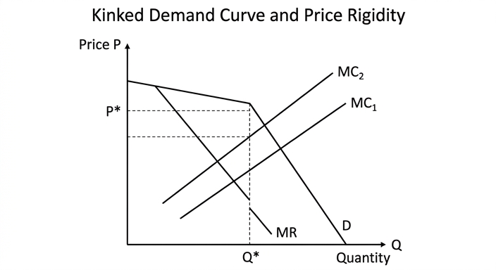
The diagram shows that even if costs change (e.g., from MC1 to MC2), the price remains at P* and quantity at Q*, so supernormal profits are maintained as long as price exceeds average cost.
Another mechanism is collusion. Firms may agree overtly or tacitly to set a high price, effectively acting as a monopoly. Game theory, particularly the Prisoner's Dilemma, shows that in a one-shot game, each firm has an incentive to cheat, but in repeated interactions, firms can sustain collusion through punishments (e.g., tit-for-tat). Where collusion is successful, supernormal profits persist.
High barriers to entry (e.g., economies of scale, patents, brand loyalty) prevent new firms from entering the market, allowing existing firms to earn supernormal profits in the long run. Even without explicit collusion, firms may engage in non-price competition (advertising, product differentiation, quality improvements) to maintain their market share and profits without engaging in price wars.
The Case Against the Statement
However, there are several factors that can undermine these abilities. First, collusion is often illegal under competition law, and even where it is not, it is difficult to sustain. The Prisoner's Dilemma highlights that cheating is individually rational, and without strong enforcement, collusion may break down, leading to price wars. The kinked demand curve model is also criticised for not explaining how the initial price is set; it only explains rigidity once price is established. Moreover, if costs change significantly, the price may need to adjust.
Second, in contestable markets, where barriers to entry and exit are low, potential competition forces firms to keep prices close to average cost, earning only normal profits. Even if the market is currently oligopolistic, the threat of entry can limit price increases and supernormal profits.
Third, non-price competition is costly. Heavy advertising and product differentiation can erode supernormal profits, reducing them to normal levels. Firms may also have objectives other than profit maximisation, such as sales maximisation or revenue maximisation, which may lead to lower prices.
Evaluation
The extent to which oligopolies can avoid price competition and maintain supernormal profits depends on the specific market conditions. In markets with high barriers to entry, effective tacit collusion, and successful non-price differentiation, the statement holds true. For example, the soft drinks industry (Coca-Cola and Pepsi) has maintained high profits through branding and limited price competition. Conversely, in markets like the airline industry, low barriers and intense price competition have forced firms to earn normal profits or losses. Additionally, government regulation and competition policy play a significant role in preventing collusive behaviour.
Conclusion
Overall, the statement is a valid generalisation for many oligopolistic markets, but it is not universally applicable. The ability to avoid price competition and maintain supernormal profits is strongest when barriers to entry are high, collusion is sustainable, and non-price competition is effective. However, when these conditions are absent, oligopolies may face price competition and only earn normal profits. Therefore, the statement is true to a large extent, but not without exceptions.
The statement is generally valid for many oligopolies, but the extent depends on market contestability, the feasibility of collusion, and the effectiveness of non-price competition. In many cases, oligopolies can avoid price competition and maintain supernormal profits, but this is not guaranteed.
Background Concept
Oligopoly is a market structure where a few firms dominate the market, leading to interdependence. Key features include high barriers to entry, product differentiation, and strategic behaviour. The kinked demand curve model explains price rigidity: firms believe rivals will match price cuts but not price rises, resulting in a demand curve with a kink at the current price. The marginal revenue curve has a vertical gap, so marginal cost can vary within that gap without affecting the profit-maximising price. Collusion, both overt and tacit, can allow firms to act like a monopoly and earn supernormal profits. Game theory, especially the Prisoner's Dilemma, illustrates the incentives to cheat and the conditions for cooperation. Barriers to entry (economies of scale, patents, brand loyalty) protect long-run profits. Non-price competition (advertising, product differentiation) is an alternative to price competition. Contestable markets theory suggests that if entry and exit are easy, the threat of entry can force firms to earn normal profits.
Understanding the Question
The question presents a statement: "Oligopolies are able to avoid price competition while maintaining supernormal profits in the long run." The command word is "Evaluate", which means we must critically assess the validity of this statement. This requires a two-sided argument: we must present evidence supporting the statement (theoretical models and real-world examples) and evidence against it (limitations and counterexamples). The essay must end with a justified conclusion that addresses the specific claim. The question is worth 20 marks, with 14 marks for AO1/AO2 (knowledge and analysis) and 6 marks for AO3 (evaluation). The top band for AO1/AO2 requires detailed knowledge, fully developed explanations, and accurate use of diagrams. The top band for AO3 requires a justified conclusion with developed evaluative comments.
Approach
To evaluate the statement, we will structure the essay as follows:
- Introduction: Define oligopoly and state the key issues.
- Arguments supporting the statement: Present the kinked demand curve model, collusion and game theory, barriers to entry, and non-price competition. Include a diagram of the kinked demand curve.
- Arguments challenging the statement: Discuss difficulties of collusion, contestable markets, costs of non-price competition, and alternative objectives.
- Evaluation: Weigh the arguments by considering market-specific conditions, such as the level of barriers, the regulatory environment, and industry characteristics. Provide real-world examples.
- Conclusion: A justified judgement that answers the question directly.
We will use the kinked demand curve diagram as a key analytical tool. The diagram will be fully explained in the text.
Step-by-Step Reasoning
Start by defining oligopoly: a market with few firms, interdependence, barriers to entry, and often product differentiation. The statement suggests that oligopolies can avoid price competition (stable prices) and still earn supernormal profits in the long run. This is a common view in economics.
Supporting Arguments:
- Kinked demand curve: Explain that each firm believes its rivals will match a price cut to avoid losing market share, but will not follow a price rise. This creates a demand curve that is kinked at the current price. The marginal revenue curve has a vertical gap. As long as the marginal cost curve (MC) passes through this gap, the profit-maximising price and quantity remain unchanged. Thus, price is sticky, and price competition is avoided. The diagram shows this: label axes, demand curve D with kink, MR with gap, MC1 and MC2 intersecting in the gap. Explain that even if costs change, the price stays the same. This allows supernormal profits to persist as long as price > average cost.
- Collusion: Firms can collude to set a high price, earning monopoly profits. Game theory: In a one-shot Prisoner's Dilemma, each firm has a dominant strategy to cheat, but in repeated games, cooperation can be sustained through strategies like tit-for-tat. Tacit collusion (price leadership) is common. Successful collusion maintains supernormal profits.
- Barriers to entry: High barriers (economies of scale, patents, brand loyalty, sunk costs) prevent new entry, so existing firms can earn supernormal profits in the long run. Without barriers, new firms would enter and drive profits down.
- Non-price competition: Instead of cutting prices, firms compete on advertising, product quality, branding, etc. This can maintain market share and profits without a price war.
Challenging Arguments:
- Collusion is often illegal (competition laws) and difficult to sustain. The Prisoner's Dilemma shows cheating is tempting; without effective punishments, collusion breaks down. Price wars can occur.
- Kinked demand curve limitations: It does not explain how the initial price is set; it only explains rigidity after price is established. If costs change significantly, the price may need to adjust. Also, empirical evidence is mixed.
- Contestable markets: If barriers to entry and exit are low, potential competition (hit and run entry) forces firms to price at average cost, earning only normal profits. Even if the market is oligopolistic, the threat of entry can limit supernormal profits.
- Non-price competition is costly: Advertising and differentiation can be expensive, eroding profits. Firms may also pursue objectives other than profit maximisation, such as sales maximisation, which may lead to lower prices.
Evaluation:
- The strength of the statement depends on the specific market. In markets with high barriers, effective tacit collusion, and successful non-price competition, the statement holds. Example: soft drinks oligopoly (Coca-Cola and Pepsi) have high brand loyalty, limited price competition, and sustained profits.
- In markets with low barriers, intense competition, or strong regulation, the statement fails. Example: airline industry, where price competition is fierce and profits are often low.
- Government policy can also break collusion (e.g., antitrust actions).
- The long-run perspective: In the long run, even high barriers can be eroded by technological change or new entrants, so supernormal profits may not be permanent.
Conclusion:
The statement is a valid generalisation but not an absolute truth. Oligopolies often can avoid price competition and maintain supernormal profits, but the extent depends on market conditions. Therefore, the statement is true to a large extent, but with important exceptions.
Key Takeaways
- Oligopoly models (kinked demand curve, collusion, game theory) provide insights into price rigidity and profit persistence.
- Evaluation requires considering the real-world conditions that affect the applicability of these models.
- Diagrams must be fully explained and integrated into the analysis.
- A justified conclusion is essential for high marks.
Common Mistakes
- Writing a one-sided answer: only supporting the statement or only challenging it. This loses all evaluation marks.
- Omitting the diagram or not explaining it. The top band requires accurate use of analytical tools and full explanation.
- Not addressing the specific statement: e.g., discussing oligopoly in general without focusing on price competition and supernormal profits.
- Lack of a conclusion or a vague conclusion that does not take a clear position.
- Using the Prisoner's Dilemma incorrectly or oversimplifying.
- Confusing short-run and long-run: it is important to distinguish that supernormal profits can persist in the long run only if barriers to entry are present.
Things to Be Careful About
- In the kinked demand curve diagram, label all axes, curves, and the gap. Explain the kink and the vertical gap in MR.
- Use real-world examples to support analysis, but ensure they are relevant to the argument.
- When discussing collusion, note that it is often illegal, but tacit collusion may still occur.
- Evaluate the statement on its own terms: avoid straying into unrelated aspects of oligopoly.
- Ensure the conclusion directly answers the question: to what extent is the statement valid?
With the help of a diagram, evaluate the consequences of imposing an effective minimum wage on the employment level and the wage level in a monopsony labour market.
Introduction
A monopsony labour market exists when there is a single buyer of labour, giving the employer market power to set wages below the competitive equilibrium. An effective minimum wage is a legally imposed floor above the current market wage. This essay evaluates the consequences of such a minimum wage on the wage level and employment in a monopsony.
Diagram and Analysis
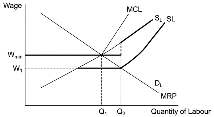
The diagram shows a monopsony labour market. The demand for labour (DL) is the marginal revenue product (MRP) curve. The supply of labour (SL) is upward sloping because the monopsonist must raise wages to attract more workers. The marginal cost of labour (MCL) lies above SL because hiring an extra worker raises the wage of all existing workers.
Without a minimum wage, the monopsonist hires where MCL = MRP, at employment Q1, and pays wage W1 on the supply curve. This is below both the competitive wage (Wc) and the competitive employment (Qc).
Now an effective minimum wage (Wmin) is imposed above W1 but not above Wc. The supply curve becomes horizontal at Wmin up to the point where the original SL reaches Wmin (at Q2). For employment beyond Q2, the supply curve follows SL. The MCL is now equal to Wmin for all workers up to Q2, because the monopsonist can hire any number of workers at the fixed minimum wage. The new MCL is horizontal at Wmin until Q2, then jumps to the original MCL.
The monopsonist now maximises profit where the new MCL (Wmin) equals MRP. This occurs at employment Q2, which is higher than Q1. The wage paid is Wmin, which is higher than W1. Thus, a moderate minimum wage can increase both the wage and the level of employment in a monopsony.
Evaluation
The outcome depends on the level of the minimum wage. If Wmin is set above the competitive wage Wc, the MCL becomes the minimum wage for all workers, and the monopsonist will reduce employment to where MRP = Wmin, which is below Qc. Thus, too high a minimum wage can reduce employment.
The elasticities of labour demand and supply matter. If labour demand is highly elastic (MRP curve flat), even a small minimum wage above W1 could lead to a large reduction in employment. Conversely, if demand is inelastic, employment may rise more.
A minimum wage may also increase labour productivity (efficiency wage effect), shifting the MRP curve rightwards, potentially increasing both wage and employment further. However, it may also raise costs, making firms less competitive internationally, or lead to substitution of capital for labour, reducing employment.
Small firms may be forced to close if they cannot afford the higher wage, reducing employment in that sector. The net effect on total employment depends on the balance between the monopsony power and these countervailing forces.
Conclusion
In a monopsony labour market, a carefully set minimum wage (not too high) can raise both wages and employment, correcting the market failure of monopsony power. However, if set too high, it can cause unemployment. The net effect is context-specific, depending on the level of the minimum wage, elasticities, and productivity responses. On balance, a moderate minimum wage is likely to be beneficial in a monopsony, but policymakers must avoid setting it above the competitive equilibrium.
A moderate effective minimum wage in a monopsony can increase both the wage level and employment, but if set too high it reduces employment; the net effect depends on the level, elasticities, and productivity responses.
Background Concept
A monopsony is a market structure with a single buyer. In the labour market, a monopsonist employer faces an upward-sloping supply curve of labour because to hire more workers it must raise the wage for all workers. This makes the marginal cost of labour (MCL) greater than the wage (the supply curve). The profit-maximising monopsonist hires labour where MCL equals the marginal revenue product (MRP) of labour, and pays the wage given by the supply curve at that employment level. This results in lower wages and lower employment than in a competitive labour market. A minimum wage is a government-imposed floor on wages. In a competitive market, a binding minimum wage above equilibrium causes unemployment. However, in a monopsony, a minimum wage can potentially increase both wages and employment by forcing the monopsonist to pay a higher wage, which also reduces its incentive to restrict employment.
Understanding the Question
The question asks you to evaluate the consequences of imposing an effective minimum wage (i.e., one that is above the current monopsony wage) on the wage level and employment level in a monopsony labour market. It explicitly requires a diagram. The command word "evaluate" means you must provide a balanced analysis of both positive and negative consequences and reach a justified conclusion. The mark scheme allocates 14 marks for AO1 (knowledge) and AO2 (analysis) and 6 marks for AO3 (evaluation). The top band for AO1/AO2 requires a detailed, fully explained diagram and developed analysis. The top band for AO3 requires a justified conclusion with developed evaluative comments.
Approach
- Start by defining monopsony and minimum wage.
- Draw and explain the standard monopsony diagram without the minimum wage, showing the monopsonist's equilibrium (W1, Q1).
- Introduce the effective minimum wage and show how it changes the supply curve and MCL. Explain the new equilibrium (higher wage and higher employment if the minimum wage is not too high).
- Analyse the impact on wage and employment: the minimum wage raises the wage directly and can increase employment because the monopsonist's MCL becomes the minimum wage, leading to a higher profit-maximising employment level.
- Evaluate: consider the level of the minimum wage (if too high, it becomes like a competitive floor and reduces employment), elasticities, productivity effects, capital substitution, firm closures, and international competitiveness.
- Conclude with a balanced judgement, noting that a moderate minimum wage can be beneficial in a monopsony but must be set carefully.
Step-by-Step Reasoning
Step 1: The monopsony model
- In a monopsony, the firm is the only employer. The supply of labour (SL) is upward sloping. The marginal cost of labour (MCL) is above SL because hiring an extra worker requires raising the wage for all workers. The demand for labour (DL) is the MRP curve.
- Profit maximisation: MCL = MRP. This gives employment Q1. The wage W1 is read off the supply curve at Q1. This is below the competitive wage Wc and employment Qc.
Step 2: Introducing an effective minimum wage
- An effective minimum wage Wmin is set above W1 but below Wc (to be effective but not too high).
- The new supply curve becomes: horizontal at Wmin up to the point where the original SL reaches Wmin (at Q2). For employment beyond Q2, the supply curve follows SL.
- The new MCL: for employment up to Q2, the MCL is constant at Wmin because each additional worker costs exactly Wmin (no need to raise wages for existing workers). At Q2, the MCL jumps to the original MCL because beyond that, the firm must raise wages for all workers.
- The new profit-maximising condition: the firm hires where the new MCL (Wmin) equals MRP. This occurs at Q2, which is greater than Q1. The wage paid is Wmin, which is higher than W1.
- Therefore, a moderate minimum wage increases both wage and employment in a monopsony.
Step 3: Evaluation
- Level of minimum wage: If Wmin is set above Wc, then the MCL becomes Wmin for all workers (since the supply curve is below Wmin, the firm can hire any number at Wmin). The firm hires where MRP = Wmin, which is below Qc. So employment falls. Thus, the outcome is sensitive to the level.
- Elasticities: If MRP is highly elastic (flat), even a small increase in wage above W1 leads to a large reduction in employment (if Wmin is above Wc). If MRP is inelastic, employment may not fall much. Similarly, the elasticity of labour supply affects the shape of MCL.
- Productivity effects: A higher wage may increase worker productivity (efficiency wage theory), shifting MRP rightwards. This could further increase employment and wages, offsetting any negative effects.
- Capital-labour substitution: If firms can easily substitute capital for labour, a higher wage may lead to automation, reducing employment.
- Firm closures: Small firms with low profit margins may be unable to pay the minimum wage and may close, reducing employment.
- International competitiveness: Higher labour costs may make firms less competitive in global markets, potentially reducing output and employment.
Step 4: Conclusion
- The net effect depends on the specific circumstances. A moderate minimum wage (below the competitive equilibrium) can correct the monopsony distortion and raise both wage and employment. However, if set too high, it can cause unemployment. The most likely outcome in a monopsony is that a well-calibrated minimum wage is beneficial, but policymakers must consider the elasticities and potential negative side effects.
Key Takeaways
- In a monopsony, the employer has market power and pays below the competitive wage.
- A minimum wage can increase both wages and employment if set at a moderate level, because it reduces the monopsonist's incentive to restrict employment.
- The diagram is crucial: it must show the original monopsony equilibrium, the minimum wage line, the new MCL, and the new equilibrium.
- Evaluation must consider the level of the minimum wage, elasticities, productivity effects, and other real-world complications.
- A justified conclusion is required for top marks.
Common Mistakes
- Drawing a competitive labour market diagram instead of a monopsony diagram. The monopsony diagram has an upward-sloping supply curve and a marginal cost curve above it.
- Forgetting to label the axes (wage and quantity of labour) and curves (SL, MCL, DL/MRP).
- Not explaining the diagram in the text; the diagram must be fully explained.
- Assuming that a minimum wage always reduces employment; in a monopsony it can increase employment.
- One-sided evaluation: only discussing benefits or only drawbacks. The question requires evaluation of consequences, so both sides must be considered.
- Conclusion that is vague or just a summary; it must be a justified judgement.
- Not addressing the specific requirement to evaluate consequences on both wage level and employment level.
Things to Be Careful About
- Ensure the diagram is accurate: the MCL curve must be steeper than the supply curve. The minimum wage line should be horizontal and intersect the MRP curve at a point to the right of the original equilibrium.
- Clearly state that the minimum wage is "effective" meaning it is above the current wage.
- Use correct terminology: monopsony, marginal revenue product, marginal cost of labour.
- In evaluation, avoid simply listing points; develop each point with reasoning.
- The conclusion should directly answer the question: what are the consequences on wage and employment? It should state under what conditions the consequences are positive or negative.
- Remember that the question asks to evaluate the consequences, not just describe them. So you must weigh up the arguments and reach a judgement.
With the help of a diagram, assess the effectiveness of government policies that might be used to reduce demand-pull inflation.
Introduction
Demand-pull inflation occurs when aggregate demand (AD) exceeds the economy's productive capacity, causing a sustained rise in the price level. It is typically illustrated by a rightward shift of the AD curve along the short-run aggregate supply (SRAS) curve. Government policies to reduce demand-pull inflation aim to decrease AD, primarily through contractionary fiscal policy and monetary policy. This essay assesses the effectiveness of these policies, with the help of a diagram.
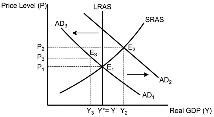
The diagram shows an initial equilibrium at price level P1 and real output Y1, with AD1 intersecting SRAS at the long-run equilibrium Y* (potential output). Demand-pull inflation shifts AD to AD2, raising the price level to P2 and output to Y2 (above Y*). Contractionary policy shifts AD to AD3, reducing the price level to P3 and output to Y3 (close to Y*). The effectiveness depends on the magnitude of the shift and the slope of SRAS.
The use of fiscal policy
Contractionary fiscal policy involves reducing government spending (G) and/or increasing taxes (T). This reduces AD directly (via G) or indirectly (via consumption and investment). For example, an increase in income tax reduces disposable income, lowering consumption and thus AD. In the diagram, this shifts AD leftwards. If the economy is near full employment, the reduction in AD can lower inflationary pressure without causing a deep recession. However, effectiveness is limited by:
- Time lags: recognition, decision, and implementation lags delay the impact.
- Perverse effects: higher taxes may reduce incentives to work and invest, harming long-run growth.
- Crowding out: lower government spending may reduce public services, affecting welfare.
The use of monetary policy
Contractionary monetary policy involves raising interest rates, reducing the money supply, or appreciating the exchange rate. Higher interest rates increase the cost of borrowing, reducing consumption and investment. They also attract foreign capital, appreciating the currency and reducing net exports. This also shifts AD leftwards. The effectiveness depends on:
- The interest elasticity of investment and consumption: if demand is interest-inelastic, the impact is small.
- The speed of transmission: changes in interest rates affect spending with a lag.
- The state of the economy: if consumer confidence is low, higher rates may have a stronger effect on reducing demand.
Evaluation
The effectiveness of these policies is not straightforward. In the short run, both fiscal and monetary policy can reduce AD and thus inflation, but they may also cause a recession (output falling below Y*) and unemployment. The cost in terms of lost output is a major drawback. Additionally, the policies may be politically unpopular, making them difficult to implement fully. The time lags involved mean that by the time the policy takes effect, the economy may have already changed, potentially causing the policy to be pro-cyclical.
Moreover, supply-side policies that increase potential output (e.g., improving productivity, deregulation) can address the root cause of demand-pull inflation by expanding the economy's capacity to produce without reducing demand. However, these take longer to have an effect.
The choice of policy also depends on the initial cause of the inflation. If it is due to excess government spending, fiscal policy may be more appropriate. If it is due to credit expansion, monetary policy is better targeted.
Conclusion
Overall, contractionary fiscal and monetary policies can be effective in reducing demand-pull inflation, but they are blunt instruments that often cause significant costs in terms of lower output and employment. Their effectiveness is limited by lags, side effects, and the risk of over-correction. A more effective approach may be a combination of demand-side policies to reduce inflation in the short run and supply-side policies to boost potential output in the long run, ensuring that the economy can grow without generating inflationary pressures.
Contractionary fiscal and monetary policies can reduce demand-pull inflation in the short run, but their effectiveness is limited by time lags, negative side effects on output and employment, and the risk of causing a recession; a combination of demand-side and supply-side policies may be more sustainable in the long run.
Background Concept
Demand-pull inflation is a macroeconomic phenomenon where the general price level rises because aggregate demand (AD) exceeds the economy's productive capacity (potential output). In the AD/AS model, it is depicted as a rightward shift of the AD curve along the short-run aggregate supply (SRAS) curve, raising both the price level and real output above the long-run equilibrium. The Phillips curve shows a short-run trade-off between inflation and unemployment: lower unemployment (higher output) is associated with higher inflation. Policies to reduce demand-pull inflation are contractionary (demand-side) policies: they aim to reduce AD. The main tools are fiscal policy (changes in government spending and taxation) and monetary policy (changes in interest rates, money supply, and exchange rates). The effectiveness of these policies depends on the size of the multiplier, the slope of SRAS, the speed of the transmission mechanism, time lags, and the side effects on output and employment. Supply-side policies that increase potential output can also help by allowing the economy to grow without generating inflation, but they work more slowly.
Understanding the Question
The question asks: "With the help of a diagram, assess the effectiveness of government policies that might be used to reduce demand-pull inflation." The command word "assess" requires a balanced evaluation, presenting both the strengths and weaknesses of the policies, and reaching a justified conclusion. The phrase "with the help of a diagram" means that a diagram is mandatory; if it is missing or not explained, the answer cannot reach the top band (L2 max if no diagram). The policies to be considered are primarily contractionary fiscal and monetary policies. The response must define demand-pull inflation, explain its causes, and then analyse how each policy works to reduce it, using the diagram to illustrate the effect. The evaluation must consider the limitations, side effects, and relative effectiveness of the policies, and conclude with a reasoned judgement.
Approach
- Define demand-pull inflation and explain its causes (e.g., rising consumer spending, investment, government spending, or net exports).
- Present the AD/AS diagram: initial equilibrium, shift to show demand-pull inflation, then shift to show the effect of contractionary policy.
- Explain contractionary fiscal policy: how it reduces AD, its strengths (direct impact on government spending, can be targeted) and weaknesses (time lags, political opposition, crowding out, negative effects on incentives).
- Explain contractionary monetary policy: how it reduces AD via interest rates, exchange rates, and money supply, and its strengths (flexibility, speed of implementation) and weaknesses (interest elasticity, transmission lags, risk of deflation, impact on investment and housing).
- Evaluate the policies by comparing them on criteria such as time lags, side effects (unemployment, recession), political feasibility, and the state of the economy.
- Conclude by weighing the relative effectiveness and suggesting when each policy might be more appropriate, and whether a combination of demand-side and supply-side policies is preferable.
Step-by-Step Reasoning
Step 1: Define demand-pull inflation
Demand-pull inflation is a rise in the general price level caused by excess aggregate demand. It often occurs when the economy is growing rapidly, above its potential output, leading to upward pressure on prices. The AD/AS model is used to illustrate this.
Step 2: Draw and explain the diagram
Start with a standard AD/AS diagram. The vertical axis is the price level (P), the horizontal axis is real GDP (Y). Draw a vertical long-run aggregate supply curve (LRAS) at Y* (potential output). Draw an upward-sloping short-run aggregate supply curve (SRAS). The initial aggregate demand curve AD1 intersects SRAS and LRAS at point E1, with price level P1 and real GDP Y1 (equal to Y*). This is the long-run equilibrium.
Now, demand-pull inflation is represented by a rightward shift of AD to AD2. This could be due to an increase in consumption, investment, government spending, or net exports. The new intersection is at point E2, with price level P2 and real GDP Y2 (above Y*). The gap between Y2 and Y* is the inflationary gap. The price level has risen from P1 to P2, showing the inflation.
To reduce inflation, the government implements contractionary policies. For example, contractionary fiscal policy (reducing G or increasing T) or contractionary monetary policy (raising interest rates) shifts AD leftwards to AD3. The new equilibrium is at point E3, with price level P3 (lower than P2 but possibly above P1) and real GDP Y3 (close to Y*). The diagram shows that the policy can reduce the price level, but it may also reduce output below Y*, causing a recession.
Step 3: Analyse fiscal policy
Contractionary fiscal policy reduces AD through two main channels: lower government spending (G) directly reduces AD; higher taxes (T) reduce disposable income, lowering consumption, and may also reduce investment. The effectiveness depends on the size of the multiplier. If the multiplier is large, the reduction in AD is amplified. However, there are significant limitations:
- Time lags: recognition lag (identifying the inflation), decision lag (legislating changes), implementation lag (effect on spending). By the time the policy takes effect, the economy may have moved into a recession, making the policy pro-cyclical.
- Political opposition: reducing G or increasing T is often unpopular, making it difficult to implement.
- Crowding out: if the government cuts spending on infrastructure, it may reduce long-term potential output.
- Negative incentives: higher taxes may reduce work effort and investment, harming long-run growth.
Step 4: Analyse monetary policy
Contractionary monetary policy reduces AD by raising the cost of borrowing (higher interest rates), reducing the money supply, or appreciating the exchange rate. Higher interest rates discourage consumption (especially on durable goods) and investment (as borrowing costs rise). They also attract foreign capital, causing the currency to appreciate, which reduces net exports. The effectiveness depends on:
- Interest elasticity of demand: if investment and consumption are insensitive to interest rates, the impact is small.
- Transmission lags: changes in interest rates take 6-18 months to affect spending fully.
- The state of the economy: if households and firms are already heavily indebted, higher rates may have a stronger effect.
- The risk of deflation: if the policy is too aggressive, it can cause a sharp fall in asset prices and deflation, worsening the recession.
Step 5: Evaluate the policies
Both fiscal and monetary policy can reduce demand-pull inflation, but they come with costs. The main trade-off is between inflation and unemployment: reducing inflation often increases unemployment. This is the short-run Phillips curve trade-off. The sacrifice ratio measures the cumulative loss of output needed to reduce inflation by 1 percentage point. The effectiveness also depends on the credibility of the policy: if the central bank is credible, expectations adjust quickly, reducing the cost of disinflation.
Monetary policy is generally more flexible and quicker to implement than fiscal policy, as central banks can change interest rates at short notice. However, fiscal policy can be more targeted (e.g., specific spending cuts). In practice, a combination of both is often used.
Supply-side policies that increase potential output (e.g., improving education, deregulation, tax reforms) can also help reduce demand-pull inflation by allowing the economy to grow faster without generating inflation. However, these take time to have an effect and are not a short-term solution.
Step 6: Conclusion
In conclusion, contractionary fiscal and monetary policies are effective in reducing demand-pull inflation in the short run, but they are blunt instruments that may cause significant economic costs in terms of lower output and higher unemployment. Their effectiveness is limited by time lags, side effects, and the risk of causing a recession. A more sustainable approach may be to use a combination of demand-side policies to bring down inflation quickly and supply-side policies to expand potential output, thereby reducing inflationary pressures in the long run. The choice of policy should depend on the specific cause of the inflation and the state of the economy.
Key Takeaways
- Demand-pull inflation is caused by excess aggregate demand and can be illustrated by a rightward shift of the AD curve in the AD/AS model.
- Contractionary fiscal and monetary policies shift AD leftwards, reducing the price level.
- The AD/AS diagram is essential for explaining the mechanism and must be fully labelled and explained.
- The effectiveness of these policies is limited by time lags, side effects (recession, unemployment), and political feasibility.
- A balanced evaluation considers both the strengths and weaknesses, and a justified conclusion is required.
- Supply-side policies can complement demand-side policies for a more sustainable solution.
Common Mistakes
- Omitting the diagram or failing to explain it: the mark scheme states L2 max if no relevant diagram.
- One-sided analysis: only discussing how policies reduce inflation without discussing the costs, or only discussing the drawbacks without showing how they work.
- Not reaching a conclusion, or providing a vague conclusion like "it depends" without specifying on what.
- Confusing demand-pull with cost-push inflation: ensure the analysis is about reducing AD, not shifting AS.
- Discussing irrelevant policies: e.g., focusing on supply-side policies without linking them to demand-pull inflation.
- Not using the diagram to support the analysis: the diagram should be referenced in the text and explained.
- Listing points without development: the top band requires developed and detailed analysis.
Things to Be Careful About
- Label the diagram fully: include axes (Price Level, Real GDP), curves (AD, SRAS, LRAS), equilibrium points, and shifts with arrows.
- Distinguish between short-run and long-run effects: e.g., the Phillips curve trade-off is short-run; in the long run, expectations adjust.
- Use precise economic terminology: e.g., "contractionary fiscal policy", "transmission mechanism", "interest elasticity".
- Consider the opportunity cost of policies: e.g., higher taxes reduce incentives, lower government spending cuts public services.
- Ensure the evaluation is developed: not just a list of points, but a reasoned weighing of the evidence.
- The conclusion must be justified: state which policy is more effective and under what conditions, and why.
- Avoid making predictions about specific numbers; stay theoretical and use the diagram to support the arguments.
With the help of a diagram, evaluate the effectiveness of the use of expenditure-switching policies to reduce a current account deficit on the balance of payments.
Introduction
A current account deficit occurs when the value of imports of goods and services exceeds the value of exports, plus net income and transfers. Expenditure-switching policies aim to shift domestic and foreign spending away from imports and towards domestically produced goods and services, thereby reducing the deficit. The two main expenditure-switching policies are protectionist measures, such as tariffs, and a devaluation or depreciation of the exchange rate. This essay evaluates the effectiveness of these policies.
The case for expenditure-switching policies
A tariff is a tax on imported goods. By raising the price of imports relative to domestic substitutes, a tariff switches expenditure towards domestic products, reducing the volume of imports and improving the current account balance.
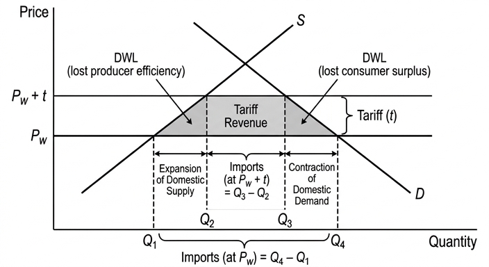
In the diagram, the domestic market for a good is shown. The world price is Pw. At this price, domestic supply is Q1 and domestic demand is Q4, so imports are Q4 – Q1. The imposition of a tariff raises the domestic price to Pw + t. Domestic supply expands to Q2, domestic demand contracts to Q3, and imports fall to Q3 – Q2. The tariff revenue is the area (Pw + t – Pw) × (Q3 – Q2). The current account improves by the value of the reduction in imports. However, the tariff also creates a deadweight welfare loss (the two triangles representing lost consumer surplus not captured by producer surplus or tariff revenue) and a net welfare loss for the importing country.
A devaluation of the currency under a fixed exchange rate system makes exports cheaper in foreign currency and imports dearer in domestic currency. If the Marshall-Lerner condition holds — that the sum of the price elasticities of demand for exports and imports is greater than one — the volume effect will dominate the price effect, and the current account will improve in the long run. In the short run, the J-curve effect may cause the deficit to worsen initially as contracts are honoured at the old exchange rate before volumes adjust.
The case against expenditure-switching policies
Tariffs are likely to provoke retaliation from trading partners, who may impose their own tariffs on the country's exports. This can reduce export volumes, offsetting any improvement in the current account and possibly leading to a trade war that leaves both countries worse off. Tariffs also raise the price of imported raw materials and components, increasing costs for domestic firms and contributing to cost-push inflation. This may force the central bank to raise interest rates, dampening investment and growth.
A devaluation is not always effective. If demand for exports and imports is price-inelastic (the Marshall-Lerner condition fails), the current account may worsen. For example, if a country imports essential raw materials with few substitutes, the volume of imports may not fall significantly despite the higher price, so the import bill rises. A devaluation also raises the domestic price of imported goods, contributing to cost-push inflation and reducing real incomes. This may lead to demands for higher wages, setting off a wage-price spiral. Furthermore, a devaluation does nothing to address the underlying causes of a deficit, such as low productivity, poor product quality, or a lack of export competitiveness.
Evaluation
The effectiveness of expenditure-switching policies depends critically on the specific circumstances. Tariffs can provide a quick, temporary improvement in the current account, but the risk of retaliation and the welfare loss make them a poor long-term solution. A devaluation is more market-based and avoids the direct welfare loss of a tariff, but its success hinges on the Marshall-Lerner condition being satisfied and on the absence of offsetting domestic inflation. In the long run, supply-side policies to improve productivity and export competitiveness are likely to be more sustainable than either tariffs or devaluation.
Conclusion
Expenditure-switching policies can be effective in reducing a current account deficit in the short to medium term, particularly a devaluation when the Marshall-Lerner condition holds and there is spare capacity in the economy. However, they are not a panacea. Tariffs carry significant risks of retaliation and welfare loss, and devaluation may fuel inflation. Their effectiveness is therefore limited and context-dependent; they are best used as part of a broader strategy that includes supply-side reforms to address the root causes of the deficit.
Expenditure-switching policies such as tariffs and devaluation can reduce a current account deficit in the short to medium term, but their effectiveness is limited by risks of retaliation, welfare loss, inflation, and the need for the Marshall-Lerner condition to hold. They are best used as part of a broader strategy including supply-side reforms.
Background Concept
A current account deficit on the balance of payments means that a country is spending more on imports of goods and services, plus net income and transfers, than it is earning from exports. This is not necessarily a problem in the short run if it is financed by capital inflows, but a persistent large deficit can lead to a loss of confidence, a depreciation of the currency, and a build-up of foreign debt.
Expenditure-switching policies aim to change the relative prices of domestic and foreign goods, so that consumers and firms switch their spending from imports to domestically produced goods. The two main types are:
- Protectionist measures (e.g., tariffs, quotas, subsidies to domestic producers) – these directly raise the price of imports or lower the price of domestic substitutes.
- Exchange rate changes (devaluation under a fixed system, or depreciation under a floating system) – these alter the relative price of domestic and foreign goods through the currency market.
The effectiveness of these policies depends on the price elasticities of demand for exports and imports, the response of trading partners, and the impact on other macroeconomic objectives such as inflation and growth.
Understanding the Question
This is a 20-mark, undivided essay from the A Level Paper 4 (2023 onwards format). The command word is "evaluate", which requires a two-sided analysis and a justified conclusion. The question asks you to assess how effective expenditure-switching policies are at reducing a current account deficit. You must:
- Define the key terms (current account deficit, expenditure-switching policies).
- Explain how at least two such policies work (tariffs and devaluation are the most obvious).
- Provide a fully labelled and explained diagram for at least one policy (the mark scheme says L2 max if no relevant diagram).
- Analyse the impact on the current account and on other stakeholders (consumers, firms, government).
- Evaluate the policies by considering their limitations, risks, and the conditions under which they work.
- Reach a justified conclusion that answers the specific question.
The top band for AO1/AO2 (11–14 marks) requires detailed knowledge, fully developed explanations, accurate use of diagrams that are fully explained, and a well-organised, coherent response. The top band for AO3 (4–6 marks) requires a justified conclusion with developed, reasoned, and well-supported evaluative comments.
Approach
- Introduction: Define the current account deficit and expenditure-switching policies. State that you will evaluate two main types: tariffs and devaluation.
- First side – the case for expenditure-switching:
- Explain how a tariff works, using a diagram to show the reduction in imports and the welfare effects.
- Explain how a devaluation works, introducing the Marshall-Lerner condition and the J-curve effect.
- Second side – the case against:
- Discuss retaliation, welfare loss, and inflation from tariffs.
- Discuss the conditions for devaluation to fail (inelastic demand, inflation, no structural improvement).
- Evaluation: Weigh the two policies against each other and against alternatives (supply-side policies). Consider the time horizon, the specific circumstances of the economy, and the trade-offs involved.
- Conclusion: Give a balanced but justified judgement on the overall effectiveness.
Step-by-Step Reasoning
Step 1: Define the current account deficit
The current account records the value of exports and imports of goods and services, plus net income and transfers. A deficit means the value of imports exceeds the value of exports. This must be financed by borrowing from abroad or by running down foreign exchange reserves.
Step 2: Explain expenditure-switching policies
These policies work by changing relative prices. A tariff makes imports more expensive, so domestic consumers switch to domestic substitutes. A devaluation makes exports cheaper for foreigners and imports more expensive for domestic residents, encouraging a switch in spending.
Step 3: Analyse a tariff
Draw a diagram of the domestic market for a good that is imported. The world price is Pw. At this price, domestic supply is Q1 and domestic demand is Q4, so imports are Q4 – Q1. A tariff of t per unit raises the domestic price to Pw + t. Domestic supply expands to Q2, domestic demand falls to Q3, and imports fall to Q3 – Q2. The current account improves by the value of the reduction in imports (the price times the reduction in quantity). The tariff also generates government revenue equal to the rectangle (Pw + t – Pw) × (Q3 – Q2). However, there is a deadweight welfare loss: the triangle of lost consumer surplus that is not captured by producer surplus or tariff revenue. This represents a net welfare loss for the country.
Step 4: Analyse a devaluation
A devaluation reduces the value of the domestic currency relative to foreign currencies. This makes exports cheaper in foreign currency and imports dearer in domestic currency. The effect on the current account depends on the price elasticities of demand for exports and imports. The Marshall-Lerner condition states that a devaluation will improve the current account if the sum of the absolute values of the price elasticities of demand for exports and imports is greater than one (|PEDx| + |PEDm| > 1). If the condition is not met, the current account may worsen.
In the short run, the J-curve effect may cause the deficit to worsen initially because contracts are already in place and volumes cannot adjust immediately. Over time, as new contracts are made, the volume effect takes over and the deficit improves.
Step 5: Evaluate the policies
Tariffs:
- Advantages: Quick to implement, can target specific sectors, generate government revenue.
- Disadvantages: Risk of retaliation from trading partners, which can reduce exports and lead to a trade war. Tariffs raise prices for consumers, reducing consumer surplus and possibly causing cost-push inflation. They also create a net welfare loss for the economy. They do not address the underlying causes of the deficit, such as low productivity.
Devaluation:
- Advantages: Market-based, avoids the direct welfare loss of a tariff, can improve competitiveness across all sectors.
- Disadvantages: Effectiveness depends on elasticities (Marshall-Lerner condition). May cause inflation as imported raw materials become more expensive. Does not address structural problems. May lead to a wage-price spiral if workers demand higher wages to compensate for higher import prices.
Step 6: Reach a justified conclusion
The effectiveness of expenditure-switching policies is context-dependent. A devaluation is generally more market-friendly and less likely to provoke retaliation than a tariff, but its success hinges on the Marshall-Lerner condition and on the economy having spare capacity to increase export production. Tariffs can provide a quick fix but carry significant risks. In the long run, supply-side policies to improve productivity, innovation, and export quality are likely to be more sustainable. Therefore, expenditure-switching policies can be effective in the short to medium term under the right conditions, but they are not a complete solution and should be part of a broader strategy.
Key Takeaways
- Expenditure-switching policies change relative prices to shift spending from imports to domestic goods.
- Tariffs reduce imports but cause welfare loss and risk retaliation.
- Devaluation improves the current account if the Marshall-Lerner condition holds, but may cause inflation.
- The J-curve effect means the deficit may worsen before it improves after a devaluation.
- Evaluation must consider the specific circumstances of the economy, including elasticities, spare capacity, and the risk of retaliation.
- A justified conclusion should weigh the pros and cons and state under what conditions the policies are most effective.
Common Mistakes
- One-sided answer: Only discussing the benefits of tariffs or devaluation without considering the drawbacks. This loses all evaluation marks.
- No diagram or an unlabelled diagram: The mark scheme explicitly caps at L2 if no relevant diagram is provided. Even if a diagram is included, it must be fully labelled and explained in the text.
- Confusing expenditure-switching with expenditure-reducing policies: Expenditure-reducing policies (e.g., contractionary fiscal/monetary policy) reduce aggregate demand and therefore imports, but they do not switch spending towards domestic goods.
- Ignoring the Marshall-Lerner condition: A devaluation is not automatically effective; the elasticities matter.
- No conclusion or a vague conclusion: The top band for evaluation requires a justified conclusion that addresses the specific question. A summary of both sides without a verdict is not enough.
- Listing many points without development: The top band requires developed and detailed analysis. It is better to develop two or three points fully than to list eight shallow ones.
Things to Be Careful About
- Label every axis and curve on the diagram: The tariff diagram must show the world price, the tariff-inclusive price, domestic supply and demand curves, and the areas for imports, tariff revenue, and deadweight loss.
- Explain the diagram in the text: Do not just draw it and move on. Walk through what it shows and how it supports your argument.
- Use the correct terminology: "Current account deficit", "expenditure-switching", "Marshall-Lerner condition", "J-curve effect", "deadweight welfare loss".
- Distinguish between short run and long run: The J-curve effect is a short-run phenomenon; the Marshall-Lerner condition applies in the long run.
- Consider the impact on other macroeconomic objectives: Inflation, growth, employment, and the distribution of income are all relevant.
- Be specific in the conclusion: State whether expenditure-switching policies are effective, under what conditions, and why. Avoid fence-sitting.