Economics 9708/43 — October/November 2024
Cambridge A-Level · A Level Data Response and Essays · worked solutions for every part, with the mark scheme
Topics Objectives and Pricing Policies of Firms · Employment and Unemployment · Economic Growth and Sustainability · The Multiplier and National Income Determination · Market Structures · Performance of Firms in Different Market Structures · +9 more
The threat from large firms
In 2021, one of the largest United States (US) technology companies averaged sales of US$1.2 billion a day. It took less than four seconds to earn US$52 000, the average American yearly salary. Three of the largest technology companies reported record breaking sales and profits. Five of the largest companies made combined profits of over US$68 billion.
They were helped by the Covid-19 pandemic that caused a huge increase in online working and shopping. The ability to work and shop online was greatly welcomed by many who were forced to stay at home.
Critics, however, worry that if this trend to large firms continues the future will be controlled by a handful of super-rich, super-powerful companies. They will dominate economic activity. This is not just bad for the economy; it is bad for consumers and bad for competition. Also, economic concentration causes unacceptable inequality. One powerful firm tried to prevent workers joining a trade union.
Their huge cash reserves mean that they could undercut possible new entrants and prevent competition. Investors will be wary of investing in possible competitors and new owners would be prepared to sell out to the dominant firms rather than try and compete.
The size of the firm gives it political power to fight any official or government intervention. Governments are beginning to be aware of this. The chair of the US body that deals with competition law said there was a range of potential risks created by the large companies. The government is aware of their ability to avoid paying taxes and their ability to dominate allows them to expand into markets for similar products.
Ten years ago, a co-founder of one of the large firms said ‘Joseph Schumpeter, the economist who used the term creative destruction would be proud’. But now that co-founder is not so sure. ‘We went from being pirates to being the navy. People may love pirates when they are young and small, but nobody likes a navy that acts like a pirate. Today’s technology giants are just like that’.
Source: The Guardian, 31 July 2021
Answer
Limit pricing is a strategy used by an incumbent firm to deter the entry of new firms into the market. The incumbent sets a price low enough (often close to average cost) that potential entrants cannot profitably enter, so the firm earns only normal profit in the short run to discourage entry.
Predatory pricing, by contrast, is a strategy used to force existing competitors out of the market. The firm sets a price below its average variable cost (or below marginal cost) in the short run, incurring losses, to drive out rivals. Once they exit, the firm raises prices to recover losses and earn supernormal profit. Predatory pricing is illegal under competition law, while limit pricing is generally not illegal but may be anti-competitive.
The key distinction lies in the objective: limit pricing aims to prevent entry, while predatory pricing aims to eliminate existing rivals. The time horizon also differs: limit pricing involves a sustained low price to deter entry, whereas predatory pricing is a temporary below-cost price to force exit.
Limit pricing deters entry; predatory pricing forces exit of existing rivals.
Background Concept
Pricing policies are strategies firms use to influence market outcomes. Limit pricing and predatory pricing are two such strategies that are often confused. Limit pricing is a barrier to entry: the incumbent firm sets a price low enough to make entry unattractive, so it sacrifices short-run profit (earns only normal profit) to prevent new competitors from entering. Predatory pricing is a strategy to eliminate existing competition: the firm sets a price below cost in the short run, incurring losses, to drive out rivals, then raises prices later to recoup losses. Both are anti-competitive, but predatory pricing is illegal in many jurisdictions because it involves deliberate losses to eliminate competition.
Understanding the Question
The question asks to ‘distinguish between’ limit pricing and predatory pricing. This means you need to explain what each is and then highlight the differences. The command word ‘distinguish’ requires you to identify the key features that separate the two concepts. You should not just define them separately; you must explicitly compare and contrast.
Approach
First, define limit pricing: state its purpose, how it works, and the short-run profit outcome. Then define predatory pricing: state its purpose, how it works, and the short-run loss. Then bring out the differences: objective (entry deterrence vs. rival elimination), time horizon (sustained vs. temporary), profit outcome (normal profit vs. loss), legal status (generally not illegal vs. illegal). Conclude with a clear distinction.
Step-by-Step Reasoning
Start with limit pricing: An incumbent firm in a market with potential entrants wants to keep them out. It sets a price just above average cost, so that it earns normal profit but any new entrant would have to produce at a higher cost (due to lack of scale) and would make a loss. This discourages entry. The price is not necessarily below cost, but it is low enough to be unprofitable for entrants. In contrast, predatory pricing is a reaction to an existing competitor. The dominant firm sets a price below its own average variable cost, knowing that it can sustain losses longer than the smaller rival. The rival, unable to cover variable costs, exits. Once the rival is gone, the dominant firm raises prices to recoup losses and earn supernormal profit. The differences are clear: limit pricing is about preventing entry, predatory pricing is about eliminating existing firms. The time horizon: limit pricing is a long-term strategy (the price is kept low continuously), while predatory pricing is a short-term strategy (temporarily below cost). The profit outcome: in limit pricing, the firm still makes normal profit (so no loss); in predatory pricing, the firm deliberately makes a loss in the short run. Legality: predatory pricing is illegal under competition law because it is an abuse of market power; limit pricing is not necessarily illegal, but it may be considered anti-competitive if it creates barriers to entry.
Why is this distinction important? Because they represent different types of anti-competitive behaviour that require different policy responses. Understanding the difference helps in analysing market power and regulation.
Key Takeaways
- Limit pricing deters entry; predatory pricing forces exit.
- Limit pricing involves normal profit; predatory pricing involves short-run losses.
- Predatory pricing is illegal; limit pricing is not always illegal.
Common Mistakes
- Confusing the two: thinking they are the same. They have different objectives.
- Thinking that both involve selling below cost. Only predatory pricing does.
- Not distinguishing the purpose: both are anti-competitive but target different stages.
Things to Be Careful About
- Use precise definitions: ‘price below average variable cost’ for predatory pricing, not just ‘below cost’.
- Mention the legal status as a distinguishing feature.
- Ensure you explicitly compare and contrast, not just define separately.
Explain whether there is any evidence in the article of these two types of pricing policy.
Answer
Yes, there is evidence of both types of pricing policy in the article.
Limit pricing: The article states that ‘investors will be wary of investing in possible competitors’ and ‘new owners would be prepared to sell out to the dominant firms rather than try and compete’. This suggests that the large firms have set prices low enough to make entry unprofitable, so potential entrants are discouraged. This is consistent with limit pricing.
Predatory pricing: The article says that the large firms ‘could undercut possible new entrants and prevent competition’. Undercutting can involve setting prices below cost to drive out new entrants, which is characteristic of predatory pricing. Although the article does not explicitly state that prices are below cost, the threat of undercutting is evidence of a potential predatory pricing strategy.
Yes, both limit pricing and predatory pricing are evidenced in the article.
Background Concept
This question requires you to apply your understanding of limit pricing and predatory pricing to the information in the extract. You need to search for phrases that indicate the use of these strategies. The extract provides specific language that aligns with the economic concepts.
Understanding the Question
The question asks to ‘explain whether there is any evidence’ of these two types of pricing policy. This means you need to identify relevant parts of the article and explain how they match the definitions. You must cover both types to get full marks.
Approach
First, recall the definitions from part (a)(i). Then scan the extract for clues. For limit pricing, look for phrases that suggest barriers to entry, such as investors being wary or owners selling out. For predatory pricing, look for phrases that suggest undercutting or driving out competition. Then explain the link.
Step-by-Step Reasoning
Read the extract: ‘Their huge cash reserves mean that they could undercut possible new entrants and prevent competition. Investors will be wary of investing in possible competitors and new owners would be prepared to sell out to the dominant firms rather than try and compete.’ The first sentence directly mentions undercutting, which is a typical predatory pricing tactic. The second sentence describes a situation where potential entrants are discouraged from even trying to compete, which is the effect of limit pricing. So both are present.
For limit pricing: The fact that investors are wary and new owners sell out indicates that the market is not attractive for new firms. This is equivalent to the incumbent setting a price that makes entry unprofitable – limit pricing.
For predatory pricing: The ability to undercut new entrants suggests that the large firms can lower prices to a level that new entrants cannot match, potentially below cost, to force them out. This is predatory pricing.
Note: The article does not explicitly say ‘below cost’, but the phrase ‘undercut’ implies a price lower than the competitor’s, which could be below cost. For the purpose of this question, it is sufficient to identify the evidence.
Key Takeaways
- Always refer to the extract when answering evidence-based questions.
- Use exact phrases from the extract to support your answer.
- Explain the link between the extract and the economic concept.
Common Mistakes
- Only identifying one type.
- Not explaining why the evidence fits the concept.
- Quoting without interpretation.
Things to Be Careful About
- Make sure you cover both types.
- The evidence for predatory pricing is weaker (since it says ‘could undercut’, not actual below-cost pricing), but it is still acceptable as evidence.
- Do not invent evidence that is not there.
Assess three possible positive effects on the macroeconomy of the huge increase in the size of the five largest technology companies.
Answer
The huge increase in the size of the five largest technology companies can have several positive effects on the macroeconomy. Three possible effects are:
1. Increase in employment and reduction in unemployment. The growth of these firms directly creates jobs within the companies, and also indirectly through their supply chains. Higher employment increases aggregate demand through the multiplier effect, leading to further job creation. This can reduce cyclical unemployment, especially if the economy is operating below full employment.
2. Increase in economic growth. The expansion of these firms contributes to an increase in aggregate demand (through investment and consumption) and also to an increase in aggregate supply (through innovation and productivity gains). This can raise the actual and potential growth rate of the economy. The article mentions record-breaking sales and profits, which indicate increased output and investment.
3. Improvement in the balance of payments. If these technology companies export their services, their growth can increase export revenues, improving the current account. The article notes that they are US-based, so their exports contribute to the US balance of payments. This can help reduce a trade deficit and strengthen the external value of the currency.
In addition, the multiplier effect amplifies these impacts. The size of the effect depends on the marginal propensity to consume and the extent of leakages. Overall, the positive macroeconomic effects can be significant, though they must be weighed against potential negative effects such as market concentration and inequality.
The growth of large technology firms can have significant positive effects on employment, economic growth, and the balance of payments, though the magnitude depends on factors such as the multiplier and the extent of leakages.
Background Concept
Macroeconomic effects of firm growth: When a large firm expands, it affects the economy through multiple channels. Directly, it hires more workers, invests in capital, and produces more output. Indirectly, it creates demand for inputs from other firms, leading to further rounds of spending via the multiplier. Additionally, if the firm is in the tradable sector, it can improve the balance of payments. These effects are captured by the aggregate demand-aggregate supply model and the multiplier concept.
Understanding the Question
The question asks to ‘assess three possible positive effects on the macroeconomy’. This means you need to identify three distinct effects, explain how they occur, and evaluate their significance. The effects must be macroeconomic, not microeconomic (e.g., don’t just talk about consumer surplus). The article provides context: large technology companies with huge sales and profits.
Approach
Choose three effects that are clearly macroeconomic: employment, growth, and balance of payments. For each, develop the chain of reasoning: how the growth of the firm leads to the effect. Include the multiplier mechanism to show the indirect effect. Then a brief assessment of the magnitude (e.g., depends on the multiplier, the state of the economy, etc.).
Step-by-Step Reasoning
Effect 1: Employment. The large firms hire more workers directly. The article says they have record-breaking sales and profits, suggesting they are expanding. More workers mean more income, which leads to higher consumption spending, creating further jobs in other sectors. This is the multiplier effect. The reduction in unemployment can be significant if the economy is in a recession with a negative output gap. The effect may be limited if the firms are highly automated and employ few workers relative to their sales.
Effect 2: Economic growth. The firms’ expansion increases aggregate demand (AD) through investment (building new facilities, buying equipment) and consumption (by employees). It also increases aggregate supply (AS) through innovation and productivity gains, shifting the LRAS curve outward. This can lead to both actual and potential growth. The article mentions that they helped the economy during Covid-19, which indicates their growth contributed to recovery. The size of the growth effect depends on the multiplier and the responsiveness of the economy.
Effect 3: Balance of payments. If the technology companies export services (e.g., cloud computing, advertising), their growth increases export earnings. This improves the current account. A stronger current account can reduce the trade deficit and support the exchange rate. The article mentions they are US-based, so they contribute to US exports. However, the effect may be offset if they also import components or if their profits are repatriated abroad.
Multiplier effect: The initial increase in spending (from investment and employment) leads to further rounds of spending, amplifying the initial impact. The formula: multiplier = 1/(1-MPC). The greater the MPC, the larger the multiplier. Leakages such as savings, imports, and taxes reduce the multiplier.
Assessment: The positive effects are real but depend on the economic context. If the economy is at full employment, the increase in AD may cause inflation rather than real growth. Also, the balance of payments effect may be small relative to the overall economy. The net effect must be considered alongside potential negative effects (market power, inequality).
Key Takeaways
- Large firms can have significant macroeconomic benefits through job creation, growth, and trade.
- The multiplier magnifies these effects.
- Assessment should consider the state of the economy and leakages.
Common Mistakes
- Describing microeconomic effects like consumer surplus or firm profits.
- Not developing the multiplier.
- Only listing effects without explaining the mechanism.
Things to Be Careful About
- Ensure effects are macroeconomic: employment (unemployment), growth, balance of payments, inflation, etc.
- Use the extract where relevant (e.g., record-breaking sales).
- Include a brief assessment of the magnitude or conditions.
The article says the growth of large firms is bad for consumers, bad for competition, and causes inequality.
Consider whether this statement can be supported by the article and by economic theory.
Answer
The statement that the growth of large firms is bad for consumers, bad for competition, and causes inequality can be supported by the article and by economic theory, but there are also arguments against it.
In support of the statement:
- The article provides evidence: profits compared to average salaries (inequality), restriction on union membership (bad for workers, part of inequality), avoidance of taxes (reduces government revenue, affecting equity), and expansion into adjacent markets (reduces competition).
- Economic theory: Large firms with market power can restrict output, raise prices, and reduce consumer choice, leading to allocative inefficiency and a loss of consumer surplus. They can erect barriers to entry, preventing competition, and may engage in anti-competitive practices. This is bad for consumers and competition. Inequality can arise from the concentration of profits and wealth among a few owners and shareholders, while workers may receive lower wages.
Against the statement:
- The article also notes that consumers welcomed the services during the pandemic, indicating that the firms provided valuable benefits. The firms helped the economy function during lockdowns.
- Economic theory: Large firms can achieve economies of scale, reducing average costs and prices. They can invest heavily in R&D, leading to innovation and dynamic efficiency. In contestable markets, even large firms may be forced to keep prices low and quality high. This can benefit consumers and may not necessarily harm competition. Moreover, the growth of firms can create jobs and increase economic growth, which can reduce inequality if the benefits are widely shared.
Conclusion: The statement is not always true. The net effect depends on the degree of market power, the contestability of the market, and the regulatory environment. In many cases, large firms can deliver significant benefits to consumers and the economy, but unchecked market power can lead to negative outcomes. Therefore, the statement should be considered with caution, and policies to promote competition and regulate market power are important.
The statement is not always true; large firms can have both negative and positive effects on consumers, competition, and inequality, and the net effect depends on market structure and regulation.
Background Concept
Large firms can have both positive and negative impacts on the economy. On the negative side, they may have market power, leading to higher prices, reduced output, and less choice. They can also increase inequality through high profits and low wages. On the positive side, they can achieve economies of scale, innovate, and provide valuable services. The contestable market theory suggests that even a single large firm may behave competitively if the threat of entry is high. The article provides a mixed picture.
Understanding the Question
The question asks to ‘consider whether this statement can be supported by the article and by economic theory’. The statement is: ‘the growth of large firms is bad for consumers, bad for competition, and causes inequality’. You need to present arguments for and against, using both the article and economic theory. Then reach a conclusion. The command word ‘consider whether’ implies a balanced evaluation.
Approach
Split your answer into two main sections: one for support, one for against. In each section, first use evidence from the article, then use economic theory. Then in the conclusion, weigh the arguments and give a justified judgement. The conclusion should not simply say ‘it depends’ but should state what it depends on and give a reasoned view.
Step-by-Step Reasoning
Support section:
- Article: The article mentions that the large firms have huge profits compared to average salaries, which suggests inequality. It also mentions that one firm tried to prevent workers joining a trade union, which is bad for workers’ bargaining power and can worsen inequality. The article says they avoid paying taxes, which reduces government ability to redistribute. They expand into adjacent markets, which can reduce competition. All these support the statement.
- Theory: In monopoly or oligopoly, firms can restrict output to raise prices, leading to higher prices and lower consumer surplus. This is bad for consumers. Barriers to entry reduce competition, and the absence of competition can lead to X-inefficiency and allocative inefficiency. The concentration of profits can increase inequality, especially if the owners are already wealthy. So theory supports the statement.
Against section:
- Article: The article says that the services were ‘greatly welcomed by many who were forced to stay at home’. This indicates that consumers benefited from the firms’ services. The firms helped the economy during the pandemic, providing essential services. This suggests they are not entirely bad for consumers.
- Theory: Large firms can benefit from economies of scale, which can lead to lower costs and lower prices for consumers. They can also invest in R&D, leading to product improvements and innovation. In contestable markets, the threat of entry can force large firms to act competitively. Moreover, large firms can create jobs and contribute to economic growth, which can reduce inequality if the benefits are spread. The dynamic efficiency gains can outweigh the static inefficiency. So theory provides counterarguments.
Conclusion: The statement is not a universal truth. The net effect depends on the specific market conditions: the degree of market power, the height of barriers to entry, the regulatory framework, and the extent to which the benefits are shared. In many cases, the positive effects can be significant, but without regulation, the negative effects can dominate. Therefore, a balanced view is needed, and policies should aim to harness the benefits while mitigating the harms.
Key Takeaways
- Always evaluate both sides of a statement.
- Use both extract evidence and economic theory.
- A conclusion must be justified, not just a summary.
Common Mistakes
- One-sided answer: only presenting arguments for or against.
- Not using the article: relying solely on theory.
- No conclusion or a vague conclusion like ‘it depends’ without explaining on what.
Things to Be Careful About
- Ensure you explicitly refer to the article when using evidence.
- The conclusion should address the specific statement, not just a general comment.
- The evaluation should be based on economic reasoning, not personal opinion.
Negative externalities of production cause market failure.
With the help of a diagram, assess the extent to which the introduction of indirect taxation is likely to address this cause of market failure.
Introduction
Negative externalities of production occur when the production of a good imposes costs on third parties not reflected in the market price. This leads to allocative inefficiency: the market produces at a level where private marginal cost (MPC) equals marginal benefit (MPB), but social marginal cost (MSC) exceeds MPB, creating a deadweight welfare loss. Indirect taxation, a Pigouvian tax, is a government intervention designed to internalise the externality by raising the private cost to match the social cost. This essay assesses the extent to which such a tax can address market failure.
The case for indirect taxation
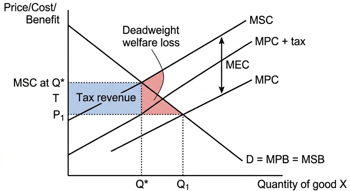
The diagram shows the market for a good with a negative production externality. The demand curve (D = MPB = MSB) represents the marginal benefit to consumers. The upward-sloping MPC curve shows the private costs of production, while the MSC curve lies above it by the marginal external cost (MEC). The market equilibrium is at output Q1 (where MPC = D), but the social optimum is at Q* (where MSC = D). The deadweight loss is the triangle between Q1 and Q* bounded by MSC and D.
An indirect tax equal to the MEC at Q* shifts the private cost curve from MPC to MPC + tax. The new supply curve now coincides with MSC, so the market equilibrium moves to Q* at a higher price P*. The tax internalises the externality: the firm pays the full social cost, output falls to the socially optimal level, and the deadweight loss is eliminated. This directly addresses the root cause of market failure — the divergence between private and social costs. In theory, if the tax is set correctly, the market outcome becomes allocatively efficient.
Limitations and counter-arguments
Despite the theoretical appeal, several practical difficulties limit the extent to which indirect taxation can fully correct the market failure. First, measuring the exact monetary value of the external cost is extremely difficult; governments often lack the information to set the tax at the precise MEC, leading to either under-correction (persistent deadweight loss) or over-correction (new inefficiency). Second, the impact of the tax depends on the price elasticity of demand for the good. If demand is inelastic (e.g., for petrol or electricity), the tax will raise price but cause only a small reduction in quantity, leaving a large external cost intact. Third, indirect taxes are regressive: they take a larger proportion of income from low-income households, raising equity concerns that may force policymakers to compromise on the tax level. Fourth, other policies such as pollution permits, regulations, or direct provision may be more effective in certain contexts — for example, permits can cap total output directly, whereas a tax might be passed on to consumers without reducing output if firms have market power. Finally, the tax can be costly to administer and enforce, and may encourage evasion or relocation of production to jurisdictions with weaker environmental standards.
Evaluation
To assess the extent of effectiveness, we must weigh the theoretical capability against the practical constraints. The indirect tax is a powerful tool when the externality is well-understood and demand is elastic; under these conditions it can achieve near-complete correction. However, informational asymmetries, inelastic demand, and equity concerns often mean the tax is set too low, resulting in only partial correction. Alternative policies like tradeable permits offer a more direct quantity control but may be less flexible. The extent also depends on the time horizon: in the long run, the tax can incentivise innovation and cleaner production methods, potentially reducing the externality further.
Conclusion
Indirect taxation can address negative externalities of production to a significant extent by internalising the external cost, but its effectiveness is limited by the difficulty of accurately measuring the externality, the regressive nature of the tax, and the availability of more direct alternatives. Therefore, the extent is moderate and context-dependent: it is most effective when the externality is measurable, demand is elastic, and the tax is combined with complementary policies. A single policy is unlikely to fully resolve market failure, but indirect taxation remains a valuable component of a broader strategy.
Indirect taxation can address negative externalities of production to a significant extent by internalising the external cost, but its effectiveness is limited by the difficulty of accurately measuring the externality, the regressive nature of the tax, and the availability of more direct alternatives; therefore, the extent is moderate and context-dependent.
Background Concept
Negative externalities of production arise when a firm's production activity imposes costs on third parties that are not reflected in the price of the good. For example, a factory emitting pollution harms the health of local residents and damages the environment. The private marginal cost (MPC) of the firm includes only the costs of inputs like labour and raw materials, while the social marginal cost (MSC) includes both the private costs and the external costs (MEC). In a free market, the firm produces where MPC = MPB (demand), leading to output Q1 that exceeds the socially optimal output Q* where MSC = MPB. The overproduction creates a deadweight welfare loss – the loss of social surplus from producing units that cost society more than they benefit consumers.
Market failure occurs because the price mechanism does not account for the full social cost; the good is under-priced and over-produced. Allocative efficiency is not achieved. Government intervention can correct this by making the producer pay the external cost, thereby aligning private and social incentives. One common policy is a Pigouvian tax – an indirect tax equal to the marginal external cost at the socially optimal output.
Understanding the Question
The question asks: "With the help of a diagram, assess the extent to which the introduction of indirect taxation is likely to address this cause of market failure." The command word is "assess" – this requires a two-sided evaluation and a justified conclusion. The specific cause of market failure is negative externalities of production. The policy is indirect taxation. The question also explicitly requires a diagram – the mark scheme caps at Level 2 if no diagram is provided. The assessment objectives are AO1/AO2 (knowledge and analysis) out of 14 marks, and AO3 (evaluation) out of 6 marks. The top band for AO1/AO2 demands detailed knowledge, fully developed explanations, and a fully explained diagram. The top band for AO3 demands a justified conclusion and developed evaluative comments.
We need to explain how the tax works in theory, then evaluate its practical limitations, and finally reach a judgement on the extent (how much it addresses the failure).
Approach
Start by defining the key concepts: negative externalities of production, market failure, allocative inefficiency, and indirect taxation. Then present the diagram: a standard negative externality diagram with MPC, MSC, D, and show the market equilibrium and social optimum. Explain how an indirect tax equal to the MEC shifts the MPC curve upward, moving the market to the social optimum and eliminating the deadweight loss. This establishes the theoretical effectiveness.
For evaluation, consider the difficulties: measurement of the external cost, the role of price elasticity of demand, regressivity, administrative costs, and alternative policies (e.g., pollution permits, regulation). Use these to argue that the extent is limited. Finally, in the conclusion, weigh the strengths and weaknesses to arrive at a balanced judgement: the tax is effective in ideal conditions but its real-world impact is partial and context-dependent.
Step-by-Step Reasoning
-
Define the problem: Negative externalities of production lead to allocative inefficiency. The market output Q1 is above the social optimum Q*. The MSC curve lies above MPC; the vertical distance is the MEC.
-
Draw the diagram:
- Axes: Quantity of good X (horizontal), Price/Cost (vertical).
- Downward sloping demand curve: D = MPB = MSB (assuming no external benefits).
- Upward sloping MPC curve.
- Upward sloping MSC curve above MPC.
- Market equilibrium: where MPC = D, at Q1, price P1.
- Social optimum: where MSC = D, at Q*, price P*.
- Shade the deadweight loss triangle between Q1 and Q* under MSC and above D.
-
Introduce the tax: An indirect tax of amount T = MEC at Q* shifts the supply curve from MPC to MPC + tax. The new supply curve now coincides with MSC. The new equilibrium is at Q* and price P* (higher than P1). The tax revenue is the rectangle between the new supply curve and the original MPC curve from 0 to Q*.
-
Explain the mechanism: The tax increases the firm's cost, so it reduces supply; price rises, quantity falls to Q*. The producer now pays the social cost, so the externality is internalised. The market failure is corrected in theory – allocative efficiency is restored.
-
Evaluate:
- Measurement difficulty: The government does not know the exact MEC; it may set the tax too low or too high. Too low leads to partial correction; too high leads to over-correction and new inefficiency.
- Price elasticity of demand: If demand is inelastic (e.g., necessities), the quantity reduction is small even with a large tax; the externality persists. The tax mainly raises revenue rather than reducing output.
- Regressivity: Indirect taxes take a larger share of income from the poor, so governments may keep the tax low to avoid political backlash, limiting its correction.
- Administrative costs and evasion: The tax may be costly to implement and enforce, especially for many small producers. Firms may relocate to avoid the tax.
- Alternative policies: Pollution permits can cap total output directly and are often more effective for large polluters. Regulations (e.g., emission standards) can be more direct but less flexible. The tax may be combined with other policies for better effect.
-
Reach a conclusion: Weigh the theoretical effectiveness against the practical limitations. The extent is moderate: the tax can address the failure significantly if well-designed, but real-world constraints mean it rarely achieves full correction. It is a useful tool but not a panacea.
Key Takeaways
- Negative externalities of production cause overproduction and deadweight loss.
- Indirect taxation (Pigouvian tax) can internalise the externality by shifting the private cost curve upward.
- A diagram is essential: show MPC, MSC, D, market equilibrium, social optimum, and the effect of the tax.
- Evaluation must consider measurement difficulty, elasticity, regressivity, and alternatives.
- A justified conclusion must state the extent and the conditions under which it works best.
Common Mistakes
- Omitting the diagram: the mark scheme caps at Level 2 if no diagram.
- Drawing a diagram without labelling axes, curves, or equilibrium points: labels are required for credit.
- One-sided answer: simply explaining the tax without evaluation (no AO3 marks).
- Vague conclusion like "it depends" without specifying what it depends on.
- Confusing negative externalities of production with consumption (e.g., smoking).
- Not relating the tax to the specific market failure: the answer must link the tax to correcting the allocative inefficiency.
- Using a generic supply and demand diagram without the MSC curve.
Things to Be Careful About
- Ensure the diagram is fully explained in the text; the examiner cannot assume the diagram speaks for itself.
- Use correct terminology: allocative efficiency, deadweight loss, marginal external cost, Pigouvian tax.
- In the evaluation, develop each point: do not just list limitations; explain why they reduce effectiveness.
- The conclusion should directly answer "to what extent" – use phrases like "to a limited extent" or "to a significant extent" and justify.
- Consider both sides: the tax can work, but it doesn't always. Balance the argument.
- Refer to the specific good mentioned in the extract (if any) – but this question has no extract, so use generic examples.
Wages in a perfectly competitive labour market will always be higher than wages in a monopsony labour market.
With the help of a diagram, evaluate this statement.
Introduction
In a perfectly competitive labour market, there are many firms demanding labour and many workers supplying labour, with perfect information and no barriers to entry. Wages are determined by the intersection of market demand (sum of firms' MRP curves) and market supply. In a monopsony labour market, there is a single buyer of labour, giving the employer market power to set wages below the competitive level. This essay evaluates whether wages in perfect competition are always higher than in monopsony, using diagrams and considering factors such as trade union and government intervention.
Perfectly competitive labour market
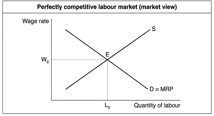
The diagram shows a perfectly competitive labour market. The market demand curve for labour (D = MRP) slopes downwards, reflecting diminishing marginal productivity. The market supply curve of labour (S) slopes upwards, reflecting the opportunity cost of work. Equilibrium wage Wc and employment Lc are determined where D = S. Each firm is a wage taker, hiring labour up to the point where the market wage equals its MRP. In the long run, workers earn a wage equal to their marginal revenue product, and there is no exploitation.
Monopsony labour market
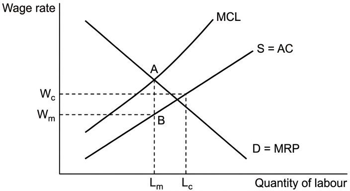
In a monopsony, the firm faces an upward-sloping supply curve of labour (S = AC of labour). The marginal cost of labour (MCL) lies above the supply curve because hiring an additional worker requires raising the wage for all existing workers. The monopsonist maximises profit by hiring labour where MCL = MRP (demand), determining employment Lm. The wage Wm is then read off the supply curve at that employment level, which is lower than the competitive wage Wc and employment Lc. This is the classic monopsony exploitation: workers are paid less than their MRP.
Evaluation
The statement that wages in perfect competition are always higher than in monopsony is not necessarily true. Several factors can alter the outcome:
-
Trade union intervention: A trade union can act as a monopoly seller of labour, bargaining for a higher wage. In a monopsony, a union can raise the wage above Wm, potentially to the competitive level or even higher, depending on bargaining power. The union may also increase productivity through training, shifting the MRP curve rightwards, which could raise wages further.
-
Government minimum wage: A legally enforced minimum wage set above Wm but below Wc can raise wages in monopsony without reducing employment (if set appropriately). In some cases, a minimum wage above the competitive wage could make monopsony wages higher than those in perfect competition.
-
Long-run adjustments: In perfect competition, if wages are high, the supply of labour may increase over time, driving wages down towards the equilibrium. In monopsony, barriers to entry may prevent such adjustments, but the monopsonist may also face competition from other firms in the long run if the market becomes contestable.
-
Productivity differences: If the monopsonist operates in a high-productivity industry (e.g., due to capital intensity), the MRP curve may be higher, leading to a higher wage even with monopsony power. Conversely, perfect competition may exist in low-productivity sectors with low wages.
-
Non-wage factors: The statement focuses on wages, but total compensation may include non-wage benefits. Monopsonists might offer lower wages but better benefits, or vice versa.
Thus, while the basic models predict higher wages under perfect competition, real-world interventions and market conditions can reverse this. The word "always" is too strong.
Conclusion
In the absence of intervention, wages in a perfectly competitive labour market are higher than in a monopsony, as the monopsonist exploits its market power to pay below MRP. However, trade union bargaining, minimum wage laws, productivity improvements, and long-run market changes can raise monopsony wages to levels that may equal or exceed competitive wages. Therefore, the statement is not always true; it depends on the presence and effectiveness of countervailing forces. A more accurate statement is that wages tend to be higher in perfect competition than in monopsony, but this is not guaranteed.
The statement is not always true; while the basic models predict higher wages under perfect competition, trade union bargaining, minimum wage laws, and productivity improvements can raise monopsony wages to equal or exceed competitive levels, so the outcome depends on the presence of countervailing forces.
Background Concept
Labour markets are factor markets where firms demand labour and workers supply labour. The wage rate is the price of labour. In a perfectly competitive labour market, many firms compete for workers, and many workers offer their labour, so no single firm or worker can influence the wage. The market wage is determined by supply and demand. Each firm hires labour up to the point where the marginal revenue product (MRP) equals the wage. In a monopsony labour market, there is only one employer (or a dominant employer) of labour in a particular area or occupation. This gives the employer market power to set wages below the competitive level because workers have few alternative job opportunities. The monopsonist faces an upward-sloping supply curve of labour, meaning to hire more workers it must raise the wage for all workers, leading to a marginal cost of labour (MCL) that is above the supply curve. The profit-maximising employment is where MCL = MRP, and the wage is determined from the supply curve at that employment, which is lower than the competitive wage.
Understanding the Question
The question presents a statement: "Wages in a perfectly competitive labour market will always be higher than wages in a monopsony labour market." It asks to evaluate this statement with the help of a diagram. The command word "evaluate" requires a two-sided analysis and a justified conclusion. The word "always" makes the statement an absolute claim, so the evaluation must challenge this absoluteness by considering conditions under which it might not hold. The question also explicitly requires a diagram, so failing to include one will cap the mark at Level 2. The essay is worth 20 marks, with 14 marks for AO1+AO2 (knowledge, understanding, analysis) and 6 marks for AO3 (evaluation). The top band for AO1+AO2 demands detailed knowledge, fully developed explanations, accurate use of diagrams fully explained, and a well-organised response. The top band for AO3 demands a justified conclusion addressing the specific requirements of the question, with developed, reasoned, and well-supported evaluative comments.
Approach
The essay should be structured as follows:
- Introduction: Define the two market structures and state the purpose of the essay.
- Analysis of perfect competition: Describe characteristics, draw and explain the diagram showing equilibrium wage and employment.
- Analysis of monopsony: Describe characteristics, draw and explain the diagram showing lower wage and employment.
- Evaluation: Discuss factors that could make wages in monopsony higher than in perfect competition. These include trade union intervention, government minimum wage, productivity differences, long-run adjustments, and non-wage compensation. Each factor should be developed with reasoning.
- Conclusion: Provide a justified judgement that addresses the "always" claim. Conclude that the statement is not always true; it depends on the presence of countervailing forces.
The diagrams must be fully explained in the prose, not just drawn. The evaluation must be two-sided: first present the case that perfect competition wages are higher (the basic model), then present the counter-case (interventions and other factors). The conclusion should weigh the arguments and give a clear verdict.
Step-by-Step Reasoning
Step 1: Perfectly competitive labour market
In a perfectly competitive labour market, there are many firms and many workers, all with perfect information. Labour is homogeneous, and there are no barriers to entry or exit. The market demand for labour is the sum of each firm's marginal revenue product (MRP) curve, which slopes downwards due to diminishing marginal productivity. The market supply of labour slopes upwards, reflecting that higher wages are needed to attract more workers into the market (the opportunity cost of leisure or alternative work). The equilibrium wage (Wc) and employment (Lc) are determined at the intersection of demand and supply. Each firm is a wage taker and hires labour up to the point where the market wage equals its MRP. In the long run, workers are paid exactly their MRP, so there is no exploitation. The diagram should show the market with D = MRP and S intersecting at Wc, Lc.
Step 2: Monopsony labour market
In a monopsony, there is a single employer of labour. The firm faces the entire market supply curve of labour, which is upward sloping. The marginal cost of labour (MCL) is greater than the average cost (the wage) because to hire an additional worker, the firm must raise the wage for all existing workers. The MCL curve lies above the supply curve. The monopsonist maximises profit by hiring labour where MCL = MRP (the demand for labour). This determines employment Lm, which is lower than Lc. The wage Wm is then read off the supply curve at Lm, which is lower than Wc. The diagram should show the supply curve (S = AC), the MCL curve above it, and the demand curve (MRP) intersecting MCL at Lm, with Wm on the supply curve at Lm. The area between Wm and the MRP at Lm represents exploitation (workers paid less than their MRP).
Step 3: Comparison
From the basic models, Wc > Wm and Lc > Lm. So the statement appears true in the absence of any other factors.
Step 4: Evaluation – factors that can reverse the outcome
-
Trade union intervention: A trade union can act as a monopoly seller of labour, bargaining for a higher wage. In a monopsony, a union can raise the wage above Wm, potentially to the competitive level or even higher. The union may also increase labour productivity through training, shifting the MRP curve rightwards, which could raise wages further. If the union is strong, wages in monopsony could exceed those in perfect competition.
-
Government minimum wage: A legally enforced minimum wage set above Wm but below Wc can raise wages in monopsony without reducing employment (if set appropriately). In some cases, a minimum wage above the competitive wage could make monopsony wages higher than those in perfect competition. However, if set too high, it could cause unemployment.
-
Productivity differences: The MRP curve depends on the productivity of labour. If the monopsonist operates in a high-productivity industry (e.g., due to advanced technology or capital intensity), the MRP curve may be higher, leading to a higher wage even with monopsony power. Conversely, perfect competition may exist in low-productivity sectors with low wages. Thus, wages in monopsony could be higher if the industry is more productive.
-
Long-run adjustments: In perfect competition, if wages are high, the supply of labour may increase over time (workers enter the market), driving wages down towards the equilibrium. In monopsony, barriers to entry may prevent such adjustments, but the monopsonist may also face competition from other firms in the long run if the market becomes contestable. However, if the monopsony is sustained, wages may remain low.
-
Non-wage factors: The statement focuses on wages, but total compensation may include non-wage benefits (health insurance, pensions, etc.). Monopsonists might offer lower wages but better benefits, or vice versa. So the comparison of wages alone may not capture the full picture.
Step 5: Conclusion
The basic models show that perfect competition yields higher wages than monopsony. However, the word "always" is too strong. Trade union bargaining, minimum wage laws, productivity differences, and other factors can raise monopsony wages to levels that may equal or exceed competitive wages. Therefore, the statement is not universally true. A more accurate statement is that wages tend to be higher in perfect competition than in monopsony, but this is not guaranteed and depends on the specific market conditions and interventions.
Key Takeaways
- Understand the characteristics and wage determination in perfectly competitive and monopsony labour markets.
- Be able to draw and explain the diagrams for both market structures, including the MCL curve in monopsony.
- Recognise that the basic model predicts higher wages in perfect competition, but real-world factors such as trade unions, minimum wages, and productivity differences can alter the outcome.
- When evaluating an absolute statement like "always", the key is to find counterexamples or conditions where it does not hold.
- A good evaluation requires developed reasoning for each factor and a justified conclusion that directly addresses the question.
Common Mistakes
- One-sided answer: Only explaining why perfect competition wages are higher without considering the counter-case. This loses all evaluation marks.
- No diagram or incorrect diagram: The mark scheme caps at Level 2 if no diagram is provided. Even if a diagram is included, it must be fully explained; a diagram without explanation is insufficient.
- Confusing monopsony with monopoly: Monopsony is a single buyer of labour, not a single seller. The diagram for monopsony is different from that for monopoly.
- Ignoring the "always": Simply stating that perfect competition wages are higher without addressing the absolute claim fails to evaluate the statement fully.
- Vague conclusion: A conclusion that just says "it depends" without specifying on what and giving a judgement is insufficient. The conclusion must be justified and address the specific question.
- Lack of development: Listing factors without explaining how they affect wages is descriptive, not analytical. Each factor should be developed with a chain of reasoning.
Things to Be Careful About
- Label diagrams clearly: Include all relevant curves (S, D=MRP, MCL, Wc, Wm, Lc, Lm). Axes should be labelled "Wage rate" and "Quantity of labour".
- Explain the MCL curve: Many students forget to draw the MCL curve or confuse it with the supply curve. Explain why MCL lies above supply.
- Use the extract? There is no extract; this is a pure essay. But if there were data, you would need to use it.
- Time management: For a 20-mark essay, allocate about 30-35 minutes. Spend time on the diagrams and evaluation.
- Real-world examples: While not required, using examples (e.g., a company town, professional sports leagues) can strengthen the evaluation.
- Avoid overgeneralisation: The statement is about wages, not employment. Keep focus on wage levels.
- Conclusion must be justified: State clearly whether the statement is true, false, or partly true, and why.
Central banks can control the money supply. An increase in the money supply will cause inflation, therefore central banks can control inflation.
Evaluate this statement.
Introduction
Inflation is a sustained increase in the general price level. The money supply (M) is the total stock of money in the economy, typically comprising currency in circulation and commercial bank deposits. The statement asserts a direct causal chain: central banks control M, an increase in M causes inflation, therefore central banks can control inflation. This essay will evaluate each link in this chain.
The case that central banks can control inflation through the money supply
The theoretical foundation is the Quantity Theory of Money (MV = PT). Assuming the velocity of circulation (V) is stable and real output (T) is at full employment, an increase in M leads directly to a proportional increase in the price level (P). For example, if M rises by 10%, P must also rise by 10% to maintain the equation. This provides a clear theoretical link.
Central banks have several instruments to control M. Open market operations (OMOs) are the primary tool: selling government securities to commercial banks reduces their reserves, contracting their ability to create credit through the bank credit multiplier. This directly reduces bank deposits, a major component of M. Quantitative tightening (the reverse of QE) works similarly by selling assets to drain reserves. Changes in the policy interest rate (e.g., Bank Rate) influence commercial banks' lending rates. Higher interest rates raise the cost of borrowing, reducing consumption and investment, which lowers aggregate demand (AD). A fall in AD reduces demand-pull inflationary pressure. Through these channels, a central bank can reduce M and/or dampen AD, thereby controlling inflation.
The case against: why the link is weak and control is imperfect
First, the money supply is difficult to define and measure. There are multiple definitions (M0, M1, M2, M4), and the relevant one for inflation is unclear. Financial innovation (e.g., new types of deposits, money market funds) blurs the boundary between money and near-money, making it hard for the central bank to target a specific aggregate accurately.
Second, the link between M and P is not stable. The velocity of circulation (V) is not constant. During a recession or a liquidity trap, V can fall sharply. An increase in M may simply be held as idle balances (hoarded) rather than spent, so AD does not rise and inflation does not occur. Conversely, if V rises unexpectedly, inflation could accelerate even without M growth.
Third, the transmission mechanism from interest rates to AD is uncertain and subject to long and variable lags. The effect of a rate change on consumption and investment depends on confidence, expectations, and the responsiveness of borrowers (interest elasticity of demand). If firms and households are pessimistic, a rate cut may not stimulate spending.
Fourth, the cause of inflation matters. The statement assumes all inflation is demand-pull. However, cost-push inflation (e.g., from rising oil prices, wage push, or supply chain disruptions) is not caused by excess M and cannot be cured by reducing M. Contractionary monetary policy to fight cost-push inflation would reduce output and employment without addressing the root cause, potentially causing stagflation.
Fifth, there are conflicts with other objectives. Raising interest rates to control inflation may cause an appreciation of the exchange rate, worsening the current account. It also reduces investment and growth, potentially increasing unemployment. These trade-offs constrain the central bank's willingness to act aggressively.
Evaluation
The strength of the central bank's control over inflation depends on the type of inflation and the economic context. For demand-pull inflation in an economy with stable velocity and well-functioning financial markets, the Quantity Theory provides a reasonable guide, and OMOs are a powerful tool. However, in a liquidity trap (as seen after 2008), QE increased the monetary base massively without causing high inflation because V collapsed. For cost-push inflation, monetary policy is largely ineffective and may do more harm than good. Furthermore, the credibility and independence of the central bank matter: if the central bank has a strong anti-inflation reputation, its announcements alone can anchor inflation expectations, reducing the need for actual changes in M.
Conclusion
The statement is an oversimplification. While central banks have the tools to influence the money supply and aggregate demand, the link between money and inflation is not deterministic. The effectiveness of monetary policy in controlling inflation is conditional on the cause of inflation (demand-pull vs. cost-push), the stability of velocity, the state of the economy (liquidity trap vs. boom), and the credibility of the central bank. Therefore, central banks can influence inflation, but they cannot fully control it in all circumstances.
Central banks can influence inflation through monetary policy, but they cannot fully control it because the link between money supply and inflation is weakened by unstable velocity, the existence of cost-push inflation, long and variable lags, and conflicts with other macroeconomic objectives. Control is strongest for demand-pull inflation in normal conditions but is severely limited during liquidity traps or when inflation is cost-push.
Background Concept
This question tests your understanding of the relationship between money, inflation, and the power of central banks. The core theoretical model is the Quantity Theory of Money, often expressed as the equation of exchange: MV = PT.
- M = Money supply (the total amount of money in the economy).
- V = Velocity of circulation (the average number of times a unit of money is spent on final goods and services in a year).
- P = Average price level.
- T = Real output (the volume of transactions, often proxied by real GDP).
The equation is an identity (it must hold true by definition), but economists make different assumptions about its components to turn it into a theory. The Monetarist view (associated with Milton Friedman) assumes that V is stable in the long run and that T is at full employment. Under these assumptions, a change in M leads to a proportional change in P. This is the theoretical basis for the claim that 'an increase in the money supply will cause inflation'.
Central banks use monetary policy to influence M and interest rates. Key instruments include:
- Open Market Operations (OMOs): Buying or selling government securities to increase or decrease bank reserves.
- Policy Interest Rate: The rate at which the central bank lends to commercial banks, which influences all other interest rates in the economy.
- Quantitative Easing (QE) / Tightening (QT): Large-scale purchases or sales of assets to directly affect the money supply and long-term interest rates when the policy rate is near zero.
The transmission mechanism describes how a change in the policy rate or M affects AD and then inflation. A typical chain is: higher policy rate -> higher commercial bank lending rates -> higher cost of borrowing -> lower consumption and investment -> lower AD -> lower demand-pull inflation.
However, the question asks you to evaluate this statement, meaning you must challenge each link in the chain. The key counter-arguments are:
- Measurement and Definition: What is 'the money supply'? There are many definitions (M0, M1, M2, M4), and financial innovation makes it hard to control a specific one.
- Velocity Instability: V is not constant. In a recession or liquidity trap, people hoard money, V falls, and an increase in M may not lead to more spending or inflation.
- Cause of Inflation: The statement assumes all inflation is demand-pull. Cost-push inflation (from supply shocks, rising wages, or import prices) is not caused by excess M and cannot be fixed by reducing M. Doing so would only reduce output and employment.
- Lags and Uncertainty: The effect of monetary policy operates with 'long and variable lags'. By the time the policy affects inflation, the economic situation may have changed.
- Conflicts: Tightening monetary policy to control inflation can cause an exchange rate appreciation (hurting exports), reduce investment (hurting long-run growth), and increase unemployment.
Understanding the Question
The question presents a three-part statement: (1) Central banks can control the money supply. (2) An increase in the money supply will cause inflation. (3) Therefore, central banks can control inflation. You are asked to 'Evaluate this statement.'
This is a classic 'evaluate' command, which requires you to do three things:
- Analyse the theoretical links (AO1/AO2).
- Challenge each link with counter-arguments and real-world complexities (AO3).
- Reach a justified conclusion that answers the specific question: to what extent is the statement true? (AO3).
The statement is an absolute claim ('will cause', 'can control'). Your evaluation should show that the reality is more conditional. The top band for AO3 requires a 'justified conclusion or judgement that addresses the specific requirements of the question' with 'developed, reasoned and well-supported evaluative comment(s).'
Approach
Your essay should be structured to systematically evaluate each part of the statement.
- Introduction: Define inflation and the money supply. State that you will evaluate each link in the chain.
- Analysis of the theoretical link (The case for):
- Explain the Quantity Theory of Money (MV=PT) and its assumptions (stable V, full employment T).
- Explain how central banks can control M (OMOs, interest rates, QE/QT).
- Explain the transmission mechanism from M/interest rates to AD to inflation.
- Evaluation of the link (The case against):
- Challenge the control of M: Measurement issues, financial innovation, the role of commercial banks in creating credit.
- Challenge the causal link from M to P: Unstable velocity (liquidity trap), the role of expectations (if people expect inflation, V may rise).
- Challenge the effectiveness of the transmission mechanism: Long and variable lags, interest inelasticity of investment, the liquidity trap.
- Challenge the assumption about the cause of inflation: Distinguish demand-pull from cost-push. Monetary policy is ineffective against cost-push.
- Challenge the 'can control' part: Conflicts with other objectives (exchange rate, growth, employment), the problem of time inconsistency, the role of central bank credibility.
- Evaluation and Conclusion: Weigh the arguments. Under what conditions is the statement more or less true? Reach a clear, justified judgement. The conclusion should not just summarise both sides but state a verdict.
Step-by-Step Reasoning
Step 1: Define key terms.
- Inflation: A sustained increase in the general price level, usually measured by the CPI or RPI.
- Money Supply (M): The total stock of money in the economy. A common definition is M2: currency in circulation plus all bank deposits (sight and time deposits).
- Central Bank: The institution responsible for monetary policy, controlling the monetary base and influencing the broader money supply.
Step 2: Explain the theoretical link (the case for the statement).
- Use the Quantity Theory of Money: MV = PT.
- Assume V is stable (determined by institutional factors like payment habits) and T is at full employment (determined by real factors like technology and labour supply).
- If M increases by 10%, and V and T are constant, then P must also increase by 10%. This is the core monetarist argument.
- Explain how central banks control M. The central bank controls the monetary base (cash + commercial bank reserves). Through the bank credit multiplier, a change in the monetary base leads to a multiple change in broad money (M2). For example, if the reserve ratio is 10%, an injection of $1bn of reserves can support up to $10bn of new deposits.
- Explain the transmission mechanism of interest rates: Higher policy rate -> higher commercial bank lending rates -> higher cost of borrowing -> lower C and I -> lower AD -> lower inflation.
Step 3: Challenge the first link: 'Central banks can control the money supply.'
- Measurement problem: There is no single 'money supply'. M0 (narrow money) is easily controlled, but M4 (broad money) is influenced by commercial bank lending decisions, which the central bank can only influence indirectly.
- Financial innovation: New financial products (e.g., money market funds, high-interest savings accounts) blur the line between money and near-money, making it hard to target a specific aggregate.
- Endogenous money: Some economists argue that the money supply is endogenous (determined by the demand for loans), not exogenous (controlled by the central bank). Banks create credit when they make loans, and the central bank accommodates the resulting demand for reserves. In this view, the central bank controls the price of reserves (interest rate) but not the quantity of broad money.
Step 4: Challenge the second link: 'An increase in the money supply will cause inflation.'
- Velocity instability: V is not constant. During the Great Recession (2008-2009), central banks engaged in massive QE, increasing the monetary base dramatically. However, V collapsed as banks hoarded reserves and households paid down debt. Inflation remained low. The equation MV=PT held, but the increase in M was offset by a fall in V, so P did not rise.
- Liquidity trap: When interest rates are near zero, the demand for money becomes perfectly elastic. An increase in M is simply held as idle balances (liquidity preference), with no effect on AD or inflation.
- Role of expectations: If the central bank increases M but people expect future inflation, they may increase spending now (V rises), causing inflation to accelerate even before the increase in M has fully worked through. Conversely, if the central bank has strong credibility, an increase in M might not cause inflation if people believe it will be reversed.
- Supply-side shocks: If inflation is caused by a rise in oil prices (cost-push), an increase in M is not the cause. Reducing M would not lower oil prices; it would only reduce output and employment, creating stagflation.
Step 5: Challenge the third link: 'Therefore central banks can control inflation.'
- Lags: Monetary policy operates with long and variable lags (typically 12-18 months). By the time the policy affects inflation, the economic situation may have changed, and the policy may be pro-cyclical rather than counter-cyclical.
- Conflicts with other objectives: Raising interest rates to control inflation may cause an appreciation of the exchange rate (attracting hot money), which worsens the current account and reduces net exports. It also reduces investment, lowering long-run growth and potentially increasing unemployment. These trade-offs may prevent the central bank from using policy aggressively enough.
- Time inconsistency: A central bank may have an incentive to create surprise inflation to reduce unemployment (short-run Phillips curve trade-off). If it succumbs to this temptation, it loses credibility, and inflation expectations become unanchored, making inflation harder to control in the long run.
- Fiscal dominance: If the government has a large debt and the central bank is pressured to keep interest rates low to reduce the cost of servicing the debt, the central bank may be unable to raise rates sufficiently to control inflation.
Step 6: Reach a justified conclusion.
- The statement is an oversimplification. The link between M and P is conditional on V being stable and the inflation being demand-pull.
- Central banks are most effective at controlling inflation when they have credibility, independence, and when inflation is clearly demand-pull. In such cases, a credible commitment to a low inflation target can anchor expectations, making the control of inflation easier.
- However, in the face of cost-push shocks, a liquidity trap, or unstable velocity, the central bank's ability to control inflation is severely limited.
- Therefore, the statement is true only under specific conditions. A more accurate statement would be: 'Central banks can influence inflation, but they cannot fully control it, especially when inflation is caused by supply-side factors or when the economy is in a liquidity trap.'
Key Takeaways
- The Quantity Theory of Money (MV=PT) is the theoretical foundation linking money supply to inflation, but its assumptions (stable V, full employment T) are often violated in the real world.
- Central banks have powerful tools (OMOs, interest rates, QE) but their control over broad money is indirect and imperfect.
- The effectiveness of monetary policy depends critically on the cause of inflation (demand-pull vs. cost-push) and the state of the economy (normal vs. liquidity trap).
- A strong evaluation requires you to challenge each link in the causal chain presented in the question, not just to describe the theory.
- A justified conclusion must state a clear verdict (e.g., 'the statement is an oversimplification') and explain the conditions under which it is more or less true.
Common Mistakes
- One-sided answer: Only explaining the Quantity Theory and how central banks control money, without any evaluation. This would score a maximum of Level 2 for AO1/AO2 and zero for AO3.
- No conclusion or a vague conclusion: Ending with 'it depends' without saying what it depends on and which way the balance lies. This would score a maximum of Level 1 for AO3.
- Confusing nominal and real variables: Forgetting that the Quantity Theory links M to P, not to real output (T). An increase in M could also increase T if the economy is below full employment.
- Ignoring the role of expectations: Not mentioning how inflation expectations can affect V and the effectiveness of policy.
- Treating all inflation as demand-pull: Failing to distinguish cost-push inflation, which is not caused by excess M and cannot be cured by reducing M.
- Overstating the central bank's control: Claiming that central banks can perfectly control the money supply, ignoring the role of commercial banks and financial innovation.
Things to Be Careful About
- Use precise terminology: 'Money supply', 'velocity of circulation', 'transmission mechanism', 'demand-pull inflation', 'cost-push inflation', 'liquidity trap', 'quantitative easing'.
- Structure your essay clearly: Use the introduction to set out the three links you will evaluate. Use separate paragraphs for the 'case for' and the 'case against'. The evaluation section should weigh the arguments, and the conclusion should provide a clear judgement.
- Depth over breadth: It is better to develop two or three strong evaluative points (e.g., velocity instability, cost-push inflation, lags) than to list five or six shallow ones.
- Answer the specific question: The question is not 'Explain how central banks control inflation.' It is 'Evaluate this statement.' Your entire essay must be structured around challenging or supporting the specific claim.
- The conclusion must be justified: Do not just restate both sides. State your verdict (e.g., 'The statement is largely true for demand-pull inflation but false for cost-push inflation') and explain why you have reached that conclusion based on the arguments you have made.
Some high-income countries have introduced a policy of high tariffs on some imports to reduce the negative effects of globalisation on their economies.
With the help of a diagram, evaluate this policy.
Introduction
Globalisation refers to the increasing integration of economies through international trade, capital flows, and the transfer of technology. For high-income countries, globalisation has brought benefits such as access to cheaper imports and larger export markets, but it has also generated negative effects, including job losses in import-competing industries, downward pressure on wages, and persistent trade deficits. In response, some high-income countries have imposed high tariffs on selected imports. This essay evaluates whether such tariffs are an effective policy to reduce these negative effects.
The case for tariffs
Tariffs are taxes on imported goods that raise their price relative to domestically produced goods. By making imports more expensive, tariffs can protect domestic industries from foreign competition, thereby preserving jobs and output in sectors that are vulnerable to globalisation.
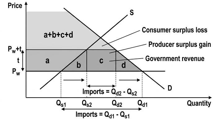
The diagram shows the domestic market for a good that is imported. The domestic demand curve is D and the domestic supply curve is S. The world price is Pw. Without a tariff, domestic production is Qs1, domestic consumption is Qd1, and imports are Qd1 – Qs1. The imposition of a specific tariff t raises the domestic price to Pw + t. Domestic production expands to Qs2, domestic consumption falls to Qd2, and imports decrease to Qd2 – Qs2. The tariff generates government revenue equal to area c (the tariff per unit multiplied by the new import quantity). Domestic producers gain producer surplus equal to area a. Consumers lose consumer surplus equal to areas a + b + c + d. The net welfare loss to the economy is the sum of the deadweight loss triangles b and d. Triangle b represents the production inefficiency caused by domestic firms producing at a cost above the world price, and triangle d represents the consumption inefficiency caused by consumers paying more and consuming less than the optimal amount.
Despite this welfare loss, the tariff may achieve other objectives. It can improve the current account by reducing the value of imports. The tariff revenue can be used to fund retraining programmes for displaced workers or to invest in industries where the country has a comparative advantage, easing the adjustment costs of globalisation. In the short run, tariffs can provide a breathing space for domestic firms to restructure and become more competitive.
The case against tariffs
However, tariffs impose significant costs. Consumers face higher prices, reducing their real purchasing power and limiting choice. The protection of inefficient domestic firms reduces the incentive to innovate and improve productivity, leading to long-run inefficiency and slower economic growth.
A major risk is retaliation. Trading partners may impose their own tariffs on exports from the high-income country, leading to a trade war that reduces export sales and harms industries that rely on global supply chains. This can offset any initial improvement in the trade balance and may even worsen it.
Tariffs also cause trade diversion. If the tariff is applied selectively, imports may shift from efficient low-cost producers to less efficient sources that are not subject to the tariff, reducing allocative efficiency. Moreover, tariffs do not address the underlying causes of globalisation’s negative effects, such as technological change that displaces labour or the natural pattern of comparative advantage. In the long run, by insulating domestic firms from competition, tariffs can reduce the dynamic gains from trade, including technology transfer and economies of scale.
Evaluation
The net effect of tariffs depends on several factors. The size of the tariff, the price elasticities of demand and supply, and the response of other countries all matter. If demand and supply are elastic, the deadweight losses are larger and the protective effect on employment is smaller. If retaliation occurs, the costs escalate.
In the short run, tariffs can cushion the impact of import competition on specific industries and workers, providing time for adjustment. However, as a permanent policy, tariffs are likely to reduce overall welfare and undermine the long-run competitiveness of the economy. The negative effects of globalisation are often concentrated in particular sectors; a more efficient approach would be to combine targeted support for affected workers (e.g., retraining, income support) with policies that enhance the economy’s flexibility and comparative advantage, rather than using broad tariffs that penalise consumers and invite retaliation.
Conclusion
While high tariffs can temporarily reduce some negative effects of globalisation, such as job losses in import-competing sectors and trade deficits, they impose substantial costs in terms of consumer welfare, productive efficiency, and the risk of trade wars. The long-run costs likely outweigh the short-run benefits, making tariffs an ineffective and potentially harmful policy for addressing the challenges of globalisation. A more sustainable strategy involves investing in human capital, innovation, and social safety nets to help workers adapt, while maintaining the benefits of open trade.
High tariffs may offer short-term protection but are generally ineffective and harmful in the long run due to inefficiency, retaliation, and loss of globalisation benefits; targeted adjustment policies are preferable.
Background Concept
Globalisation is the process of increasing economic integration between countries, driven by trade liberalisation, capital mobility, and technological advances. For high-income countries, globalisation has led to benefits such as lower consumer prices, access to a wider variety of goods, and opportunities for firms to export and invest abroad. However, it also creates negative effects: import competition can cause job losses in manufacturing sectors, downward pressure on wages for low-skilled workers, and trade deficits. These negative effects are often concentrated in specific regions and industries, leading to political pressure for protectionist measures.
Tariffs are taxes on imports that raise the domestic price of foreign goods. They are a form of protectionism intended to shield domestic industries from foreign competition. The standard microeconomic analysis of a tariff uses a supply and demand diagram for a single market. The tariff creates a wedge between the world price and the domestic price, leading to changes in production, consumption, and trade. The welfare effects include a loss of consumer surplus, a gain in producer surplus, government revenue, and deadweight losses representing the net cost to society.
The evaluation of tariffs requires considering both the intended benefits (protecting jobs, improving the trade balance) and the unintended costs (higher prices, inefficiency, retaliation). The net effect depends on the specific circumstances, including the elasticities of demand and supply, the size of the tariff, and the response of trading partners.
Understanding the Question
The question asks: "Some high-income countries have introduced a policy of high tariffs on some imports to reduce the negative effects of globalisation on their economies. With the help of a diagram, evaluate this policy."
This is a 20-mark essay from Paper 4, assessed using levels-based marking (AO1+AO2 out of 14, AO3 out of 6). The command word "evaluate" requires a two-sided analysis and a justified conclusion. The phrase "with the help of a diagram" means a diagram is mandatory; the mark scheme states that L2 is the maximum if no or incorrect diagram is provided.
The question is specific: it asks about high-income countries using high tariffs on some imports to reduce the negative effects of globalisation. Therefore, the answer must focus on the context of high-income countries and the specific negative effects of globalisation (e.g., job losses, trade deficits), not just a general discussion of tariffs.
The top band descriptors require: detailed knowledge and understanding, fully developed explanations, analysis that is developed and detailed, accurate and relevant use of analytical tools (diagram) fully explained, and a justified conclusion with developed evaluative comments.
Approach
The essay will be structured as follows:
- Introduction: Define globalisation and its negative effects on high-income countries. State the purpose of the essay.
- The case for tariffs: Explain how tariffs can reduce negative effects. Use the tariff diagram to illustrate the microeconomic effects. Discuss potential benefits: protecting jobs, improving the current account, generating revenue for adjustment assistance, providing time for restructuring.
- The case against tariffs: Discuss the costs: higher consumer prices, protection of inefficiency, risk of retaliation and trade wars, trade diversion, failure to address root causes, long-run loss of competitiveness.
- Evaluation: Weigh the arguments using criteria such as time period (short-run vs long-run), elasticities, likelihood of retaliation, and availability of alternative policies. Consider the net effect.
- Conclusion: Provide a justified judgement on whether high tariffs are an effective policy to reduce the negative effects of globalisation.
The diagram will be a standard tariff diagram, fully explained in the text.
Step-by-Step Reasoning
Introduction
Start by defining globalisation: the increasing integration of economies through trade, capital flows, and technology. For high-income countries, globalisation has led to benefits such as lower prices and export opportunities, but also negative effects: import competition can cause job losses in manufacturing, downward pressure on wages, and trade deficits. The question asks whether high tariffs on some imports can reduce these negative effects. The essay will evaluate both sides.
The case for tariffs
Tariffs raise the price of imported goods, making domestic goods relatively cheaper. This can protect domestic industries and jobs. Use the diagram to show the effects.
Explain the diagram step by step:
- Draw a domestic market for a good that is imported. Label axes Price and Quantity.
- Draw downward-sloping demand curve D and upward-sloping supply curve S.
- Show world price Pw as a horizontal line. At Pw, domestic production is Qs1, domestic consumption is Qd1, imports = Qd1 - Qs1.
- With a tariff t, domestic price rises to Pw+t. Domestic production increases to Qs2, consumption falls to Qd2, imports fall to Qd2 - Qs2.
- Consumer surplus falls by area a+b+c+d. Producer surplus rises by area a. Government gains revenue area c. Deadweight loss = b+d.
Explain the welfare loss: triangle b is the production inefficiency (domestic firms produce at cost above world price), triangle d is consumption inefficiency (consumers pay more and consume less than optimal). The net welfare loss is b+d.
Despite this loss, the tariff may achieve other objectives:
- It reduces imports, improving the current account balance.
- It protects jobs in import-competing industries, reducing unemployment.
- The tariff revenue can be used to fund retraining programmes or invest in infrastructure, helping the economy adjust.
- In the short run, it gives domestic firms time to restructure and become more competitive.
The case against tariffs
- Consumers pay higher prices, reducing real incomes and consumer surplus. This disproportionately affects lower-income households.
- Protected domestic firms have less incentive to innovate and cut costs, leading to X-inefficiency and long-run decline in competitiveness.
- Retaliation: trading partners may impose tariffs on the country's exports, reducing export sales and harming industries that rely on global supply chains. This can lead to a trade war, reducing overall trade and welfare.
- Trade diversion: if tariffs are selective, imports may shift from efficient low-cost producers to less efficient sources not subject to the tariff, reducing allocative efficiency.
- Tariffs do not address the root causes of globalisation's negative effects, such as technological change or comparative advantage. They may merely postpone adjustment.
- In the long run, by reducing competition, tariffs can lead to higher costs, lower productivity, and slower economic growth.
Evaluation
To evaluate, we need to weigh the benefits against the costs.
- Time period: In the short run, tariffs can cushion the impact of import competition, providing time for workers to retrain and firms to adjust. However, if tariffs become permanent, the costs accumulate and the economy becomes less dynamic.
- Elasticities: If demand and supply are elastic, the deadweight losses are larger and the protective effect on employment is smaller. The tariff is more costly when consumers and producers are responsive to price changes.
- Retaliation: The likelihood of retaliation depends on the importance of the trading relationship. If the high-income country is a major market, retaliation may be limited; but if it is a large economy, other countries may respond, leading to a trade war that harms both sides.
- Alternative policies: Instead of tariffs, the government could use targeted policies such as retraining programmes, income support, investment in education and infrastructure, and policies to enhance competitiveness. These can address the negative effects of globalisation without the costs of protectionism.
- Net effect: The deadweight loss from the tariff is a direct cost, while the benefits (job protection, revenue) are often temporary and may be achieved more efficiently through other means. The risk of retaliation and long-run inefficiency suggests that tariffs are not an effective long-term solution.
Conclusion
Based on the evaluation, high tariffs may provide short-term relief but are likely to be ineffective and harmful in the long run. The costs in terms of consumer welfare, inefficiency, and retaliation outweigh the temporary benefits. A more sustainable approach is to combine open trade with domestic policies that help workers and firms adapt to globalisation.
Key Takeaways
- Globalisation has both benefits and negative effects for high-income countries.
- Tariffs are a protectionist policy that can reduce imports and protect domestic industries, but they impose welfare losses.
- The standard tariff diagram shows the microeconomic effects: consumer loss, producer gain, government revenue, deadweight loss.
- Evaluation requires considering both sides: short-run benefits vs long-run costs, elasticities, retaliation, and alternative policies.
- A justified conclusion should weigh the net effect and may favour alternative policies over tariffs.
Common Mistakes
- One-sided answer: only discussing benefits or only costs. This loses all evaluation marks.
- No diagram or incorrect diagram: the mark scheme caps at L2 if no diagram.
- Diagram not explained: the top band requires diagrams to be fully explained; simply drawing it without discussing what it shows loses marks.
- Vague conclusion: "It depends" without stating what it depends on and which side is stronger.
- Not addressing the specific question: discussing tariffs in general without linking to globalisation and high-income countries.
- Ignoring retaliation: a key counter-argument that must be included.
- Treating tariffs as always bad: need to acknowledge potential short-run benefits.
Things to Be Careful About
- Label all axes, curves, and equilibrium points in the diagram.
- Explain the diagram in the prose: what shifts, what happens to price and quantity, and what the welfare areas represent.
- Use economic terminology correctly: consumer surplus, producer surplus, deadweight loss, allocative efficiency, trade diversion, retaliation.
- Ensure the conclusion is justified: state which side is stronger and why, based on the analysis.
- Avoid fence-sitting: the conclusion should take a clear position, even if conditional.
- Consider the context: high-income countries may have different elasticities and institutional capacity to implement alternative policies.