Economics 9708/42 — October/November 2024
Cambridge A-Level · A Level Data Response and Essays · worked solutions for every part, with the mark scheme
Topics Economic Growth and Sustainability · Demand for and Supply of Labour · Wage Determination and Labour Market Intervention · Balance of Payments and Policies to Correct Disequilibrium · Employment and Unemployment · Utility Theory · +4 more
Reduced Migration to the United States (US)
The factors of production land, labour, capital and enterprise form the basis for all economic output. Whilst land is geographically fixed, the other factors of production, for example labour, are mobile. Large numbers of migrants move from country to country every year. Many migrate to the US.
The average increase in the number of migrants working in the US was 0.6 million per year until 2018. However, the Covid-19 restrictions in place since 2019 prevented migration and by 2022 the total number of migrants working in the US was nearly 2 million lower than expected.
Half of migrants initially come as students, to be college educated, often in science-based subjects. Post-graduation, they often remain to work in the high-tech industries, before many return to their home countries with enhanced skills.
Well-educated immigrants are three times more likely to start businesses than inhabitants of the US. The reduction in the number of new migrants would reduce the number of new businesses and this, in turn, would reduce job creation by an estimated 200 000.
The remaining non-college educated migrants work mainly in lower-paid sectors such as retail and agriculture. They also play an important role in industries such as hospitality and food-related services. Many of the migrants send money to family members who remain in their home countries.
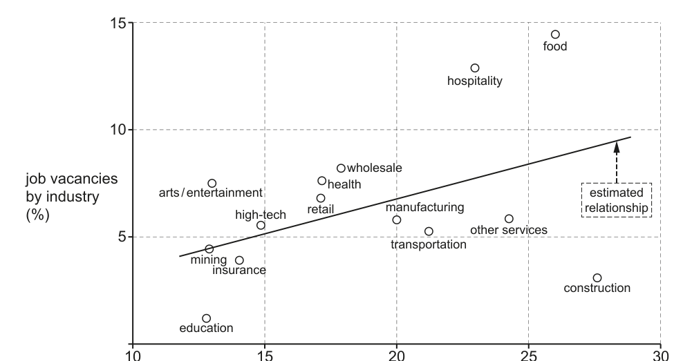
Fig. 1.1 shows the relationship between job vacancies in various industries and the share of migrant workers in the workforces of these industries in the US.
Source: US Bureau of Labor Statistics and Current Population Survey, US Census Bureau
Fig. 1.1: Unfilled job vacancies (%) and migrant workers in the workforce (%)
for selected US industries, 2019
The reduction in migrants took place at the same time as more older US workers retired.
Mexicans and Central Americans form the largest share of migrants, at over 35% of the total. Average incomes in their home countries are between 10% and 20% of the US average. There is also significant unemployment and under-employment in their home countries. In the US, migrants earn on average 12% less than the average wage for all workers. This varies by ethnic origin: Hispanic workers earn 16% less than the average while white workers earn 15% more than average.
Sources: G Peri and R Zaiour, University of California, Davis. The EconoFact Network, Statista.com N Ward and J Batalova, Migration Policy Institute, 14 March 2023
Identify the relationship between the variables shown in Fig. 1.1 and suggest one possible reason for the relationship.
Answer
There is a positive (direct) correlation between the two variables: as the share of migrant workers in an industry’s workforce increases, the percentage of unfilled job vacancies in that industry also increases.
A possible reason for this relationship is that industries with higher labour shortages (higher job vacancies) recruit more migrant workers to fill these roles, as domestic workers may be unwilling or unavailable to take these jobs.
Positive correlation; industries with higher vacancies recruit more migrant workers to fill labour shortages.
Background Concept
A scatter plot is a graphical tool used to show the relationship between two numerical variables. A positive (direct) correlation means that as one variable increases, the other also tends to increase, indicated by an upward-sloping line of best fit. In labour markets, the supply of labour to an industry depends on factors such as wage rates, skill requirements, and the availability of domestic workers. Migrant workers often supply labour to sectors where there are shortages of domestic workers, as they may be willing to take roles that domestic workers are unwilling to fill, or have skills that are in short supply domestically.
Understanding the Question
This 2-mark part asks you to first identify the relationship between the two variables shown in Fig. 1.1: the share of migrant workers in an industry’s workforce (x-axis) and the percentage of unfilled job vacancies in that industry (y-axis). You then need to suggest one plausible economic reason for this relationship. The command word "identify" requires you to state the trend clearly, and "suggest" means you need to provide a logical, economically sound reason, not a random guess.
Approach
First, observe the line of best fit in Fig. 1.1: it slopes upwards from left to right, which tells you the relationship is positive. Then, link this to labour market theory: industries with more vacancies have higher demand for labour, so they recruit more migrant workers to fill those gaps, as domestic labour supply may be insufficient. You do not need to overcomplicate the reason – a simple, logical link between vacancies and migrant recruitment is enough for 2 marks.
Step-by-Step Reasoning
- Identify the relationship: The line of best fit in Fig. 1.1 has a positive slope, meaning there is a direct (positive) correlation between the two variables: as the share of migrant workers in an industry’s workforce increases, the percentage of unfilled job vacancies in that industry also tends to increase.
- Suggest a reason: Industries with higher numbers of unfilled vacancies have excess demand for labour. To fill these gaps, firms in these industries recruit more migrant workers, who are often willing to take roles that domestic workers are unwilling or unable to fill, or who have the specific skills required for the role. This leads to a higher share of migrant workers in industries with higher vacancy rates.
Key Takeaways
- A positive correlation in a scatter plot means both variables move in the same direction.
- Migrant labour often fills gaps in sectors with domestic labour shortages, linking vacancy rates to migrant employment shares.
Common Mistakes
- Stating the relationship is negative or neutral: this would earn 0 marks for the first part.
- Giving a reason unrelated to the labour market (e.g. "migrants prefer those industries because of the weather") – this would not earn credit for the second mark.
- Confusing correlation with causation: the question only asks for a possible reason, so you do not need to prove causation, just provide a plausible link.
Things to Be Careful About
- Make sure you clearly state the relationship is positive, not just describe the graph.
- Ensure your reason is explicitly linked to the labour market, as the variables are about employment and vacancies.
With the help of a production possibility curve (PPC) diagram, explain both the likely effect of the prevention of migration to the US from 2019 and the retirement of older US workers on the US’s productive potential.
Answer
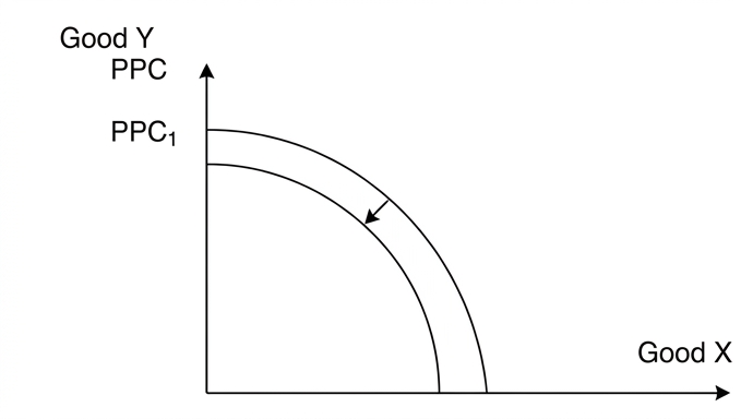
The production possibility curve (PPC) illustrates an economy’s productive potential: the maximum output of two goods it can produce when all resources, including labour, are fully and efficiently utilised.
The prevention of migration to the US from 2019 means the labour force does not grow as previously expected. This does not cause the PPC to shift inward; rather, it means the PPC does not shift outward as much as it would have done with normal migration levels, so productive potential is lower than it would have been.
The retirement of older US workers reduces the current size of the available labour force, a key factor of production. This shifts the PPC inward (to the left, from PPC to PPC1), as the economy now has fewer resources to produce goods and services, reducing its productive potential.
Prevented migration stops the PPC shifting outward as much as expected; retirement of older workers shifts the PPC inward, reducing productive potential.
Background Concept
The production possibility curve (PPC) is a macroeconomic diagram that shows the maximum possible output combinations of two goods or services an economy can produce when all its resources (land, labour, capital, enterprise) are fully and efficiently employed. The position of the PPC reflects the economy’s productive potential: an outward shift means the economy can produce more of both goods (higher productive potential), while an inward shift means it can produce less (lower productive potential). Changes in the quantity or quality of factors of production, such as the size of the labour force, will shift the PPC.
Understanding the Question
This 4-mark part asks you to use a PPC diagram to explain two separate effects on the US’s productive potential: (1) the prevention of migration to the US from 2019, and (2) the retirement of older US workers. The command word "explain" requires you to link each event to a change in the PPC, with clear reasoning. The question explicitly requires a PPC diagram, so you must include one and explain what it shows to earn full marks.
Approach
First, draw a correctly labelled PPC with two curves: the original PPC and an inward-shifted PPC1. Then, explain the two effects separately:
- Prevention of migration: this reduces the growth of the labour force, so the PPC does not shift outward as much as it would have with normal migration. It does not shift inward, because the existing labour force is still available.
- Retirement of older workers: this reduces the current size of the labour force, so the PPC shifts inward (to PPC1), as there are fewer workers available to produce goods and services.
Step-by-Step Reasoning
- Draw the PPC: Label the vertical axis "Good Y" and the horizontal axis "Good X". Draw the original PPC as a concave curve from the y-axis to the x-axis, showing the maximum output combinations when all resources are fully employed. Draw a second curve, PPC1, inside the original PPC, closer to the origin, to show an inward shift. Add an arrow pointing from the original PPC to PPC1 to show the direction of the shift.
- Effect of prevented migration: Normal migration would have increased the size of the US labour force over time, shifting the PPC outward as more workers are available to produce goods and services. The prevention of migration means this outward shift does not happen, so the US’s productive potential is lower than it would have been. However, this does not reduce the current labour force, so the PPC does not shift inward.
- Effect of retiring older workers: Older US workers leaving the workforce reduces the current quantity of labour available, a key factor of production. With fewer workers, the economy cannot produce as much output as before, so the PPC shifts inward to PPC1, reflecting a lower productive potential.
Key Takeaways
- The PPC shows an economy’s maximum possible output when all resources are fully and efficiently employed.
- A reduction in the size of the labour force shifts the PPC inward, reducing productive potential.
- A reduction in the growth of the labour force stops the PPC from shifting outward, but does not shift it inward.
Common Mistakes
- Drawing the PPC shifting outward for prevented migration: this is incorrect, as prevented migration reduces labour force growth, not the current labour force.
- Failing to distinguish between the two effects: the question asks for both, so you must explain each separately.
- Forgetting to label the axes and curves: unlabelled diagrams will lose marks.
Things to Be Careful About
- Make sure the inward shift is clearly shown on the diagram, with correct labels for PPC and PPC1.
- Explicitly state that prevented migration does not shift the PPC inward, only stops it from shifting out as much as it would have.
Using the information and labour market theory, analyse why the wages received by migrant workers in the high-tech industries are likely to be higher than the wages received by migrant workers in the hospitality industry.
Answer
Wages are determined by the interaction of the demand for and supply of labour in each industry, with the equilibrium wage equal to the marginal revenue product (MRP) of labour, adjusted by supply-side factors.
On the demand side, the MRP of migrant workers in high-tech industries is higher than in hospitality. High-tech industries produce high-value output (e.g. software, advanced technology), so the marginal product of labour (MPL) – the extra output from an additional worker – is high, and the marginal revenue (MR) from that output is also high, leading to a high MRP. Firms are willing to pay higher wages because each additional worker adds more to revenue than in low-productivity hospitality roles. In contrast, hospitality workers produce lower-value services, so their MPL and MR are lower, leading to a lower MRP and lower equilibrium wage.
On the supply side, high-tech migrant workers are typically college-educated with high skills, so their supply is relatively inelastic: there are fewer migrant workers with the required skills, so firms must pay higher wages to attract them. Hospitality migrant workers are often non-college educated, with a more elastic supply: there are more workers with the basic skills required for hospitality roles, so wages are lower. Additionally, the text notes that well-educated migrants are more likely to start businesses, capturing high profits, which further increases the returns to skilled migrant workers in high-tech.
High-tech migrant workers have higher MRP due to higher productivity and output value, and a more inelastic supply due to scarce skills, leading to higher equilibrium wages than hospitality migrant workers.
Background Concept
In a competitive labour market, the equilibrium wage rate is determined by the intersection of the demand for labour and the supply of labour. The demand for labour is a derived demand, based on the productivity of workers: firms will pay a wage equal to the marginal revenue product (MRP) of labour, which is the extra revenue a firm earns from hiring an additional worker. MRP is calculated as the marginal product of labour (MPL, extra output from an additional worker) multiplied by the marginal revenue (MR, extra revenue from selling that extra output). The supply of labour depends on factors such as the skill level of workers, the number of workers available with the required skills, and the wage rate offered. Wage differentials between industries arise because of differences in the MRP of labour and differences in the elasticity of supply of labour to different sectors.
Understanding the Question
This 6-mark part asks you to use labour market theory to explain why migrant workers in the US high-tech industry earn higher wages than migrant workers in the hospitality industry. The command word "analyse" requires you to build a full causal chain, using both demand-side (MRP) and supply-side factors, and link your reasoning to the information in the text (e.g. skill levels of migrants in different sectors).
Approach
Structure your answer around demand and supply side factors:
- Demand side: Use MRP theory to explain why high-tech workers have a higher MRP than hospitality workers, leading to higher demand and higher wages.
- Supply side: Explain how the skill level and elasticity of supply of migrant workers differ between the two sectors, leading to different equilibrium wages.
- Link to the text: Use the information that high-tech migrants are college-educated, while hospitality migrants are often non-college educated, to support your points.
Step-by-Step Reasoning
- Demand-side explanation: The demand for labour is equal to the MRP of workers. In the high-tech industry, migrant workers are often college-educated in science-based subjects, so their marginal product of labour (MPL) is high: they produce high-value output (e.g. software, advanced technology) that generates high marginal revenue for firms. This leads to a high MRP, so firms are willing to pay higher wages to attract these workers. In contrast, hospitality workers (e.g. in hotels, restaurants) produce lower-value services, so their MPL and MR are lower, leading to a lower MRP and lower equilibrium wage.
- Supply-side explanation: The supply of labour to an industry depends on the number of workers willing and able to work in that sector at different wage rates. High-tech migrant workers have rare, high-level skills, so the supply of these workers is relatively inelastic: there are few migrant workers with the required qualifications, so firms must offer higher wages to attract them. Hospitality migrant workers often have basic skills that are more widely available, so the supply of labour to hospitality is relatively elastic: there are many workers who can perform these roles, so firms do not need to offer high wages to fill vacancies. The text also notes that well-educated migrants are more likely to start businesses, capturing high profits, which further increases the returns to skilled migrant workers in high-tech.
- Additional factor: The text notes that Hispanic migrant workers (who are over-represented in low-skilled sectors like hospitality) earn 16% less than the average wage, while white migrant workers (who are more likely to work in high-skilled sectors) earn 15% more than average. This suggests that discrimination based on ethnic origin may also contribute to wage differentials between sectors.
Key Takeaways
- Wages are determined by the intersection of labour demand (based on MRP) and labour supply.
- Higher-skilled workers have a higher MRP and more inelastic supply, leading to higher wages.
- Wage differentials between sectors arise from differences in worker productivity and the availability of skilled labour.
Common Mistakes
- Only explaining one side (demand or supply): you need to cover both to earn full marks for 6 marks.
- Failing to link your reasoning to the text: you must use the information about migrant skill levels in different sectors to support your points.
- Confusing MRP with marginal profit: MRP is marginal revenue product, not marginal profit, so you must link it to revenue, not profit (though the text mentions entrepreneurs earning profits, which is a valid additional point).
Things to Be Careful About
- Make sure you clearly distinguish between high-tech and hospitality workers when explaining each point.
- If you use a labour market diagram, make sure to label the axes (wage rate, quantity of labour), the demand (D) and supply (S) curves, and the equilibrium wage for each sector, and explain what the diagram shows.
Evaluate the likely impact of a return to the migration levels prior to 2019 on the macroeconomic performance of the US economy.
Answer
Returning to pre-2019 migration levels would have mixed effects on US macroeconomic performance, with net benefits for growth and employment but a likely negative impact on the balance of payments.
On the positive side, increased migration would expand the labour force, shifting the long-run aggregate supply (LRAS) curve to the right, raising the economy’s productive potential and supporting higher actual economic growth. Migrants are likely to have a high marginal propensity to consume (MPC), so their spending would increase aggregate demand (AD), with a strong multiplier effect further boosting output and employment. The text notes that migrants are concentrated in sectors with high job vacancies (e.g. hospitality, food, high-tech), so increased migration would reduce unfilled vacancies, lowering unemployment. Additionally, well-educated migrants are three times more likely to start businesses, which would increase job creation by an estimated 200,000, further supporting employment and innovation-led growth.
On the negative side, migrants send remittances to family members in their home countries, which is a leakage from the US circular flow of income. This would reduce net exports (X - M), worsening the current account balance of payments. There is also a risk that migrant workers could crowd out domestic workers in low-skilled sectors, though the text notes that migrants often fill vacancies that domestic workers are unwilling or unable to take, so this effect is likely to be limited.
Overall, the positive effects on economic growth and employment are likely to outweigh the negative effect on the balance of payments, as the US has a strong track record of using migrant labour to support growth without significant domestic employment losses. The government would be better able to achieve its core macroeconomic objectives of growth and low unemployment, even if the current account deficit worsens slightly.
Returning to pre-2019 migration levels would improve US macroeconomic performance overall, as the benefits to economic growth and employment outweigh the small negative effect on the balance of payments.
Background Concept
Macroeconomic performance is measured against key government objectives: high and stable economic growth, low unemployment, low and stable inflation, and a balanced balance of payments. Changes in factors such as the size of the labour force, aggregate demand, and aggregate supply will affect these objectives, often creating trade-offs between them. Migration affects the economy through both supply-side (labour force size, productivity) and demand-side (migrant spending, remittances) channels.
Understanding the Question
This 8-mark evaluative part asks you to assess the likely impact of returning to pre-2019 migration levels on US macroeconomic performance. The command word "evaluate" requires you to analyse both the positive and negative effects of increased migration on macroeconomic objectives, weigh these against each other, and reach a justified conclusion. You must use the information in the text to support your points, and the mark scheme reserves 1 mark for a justified conclusion.
Approach
Structure your answer around the main channels through which migration affects macro performance, covering both positive and negative effects:
- Positive effects: impact on aggregate supply (productive potential, growth), aggregate demand (multiplier, output, employment), and job creation from migrant entrepreneurship.
- Negative effects: impact on the balance of payments from remittances, and the potential for crowding out of domestic workers.
- Evaluation: weigh the positive effects against the negative effects, considering the relative importance of each objective for the US, and the evidence in the text about migrant workers filling vacancies rather than taking domestic jobs.
- Conclusion: state a clear, justified judgement on the net impact of returning to pre-2019 migration levels.
Step-by-Step Reasoning
- Positive effect 1: Increased migration expands the labour force, which is a key factor of production. This shifts the long-run aggregate supply (LRAS) curve to the right, increasing the economy’s productive potential and supporting higher long-run economic growth. It also increases short-run aggregate supply (SRAS), as more workers are available to produce goods and services, which can help stabilise prices (reduce inflationary pressures) by increasing the economy’s capacity to meet demand.
- Positive effect 2: Migrants spend their income in the US economy, increasing consumption, a component of aggregate demand (AD). Migrants often have a high marginal propensity to consume (MPC), as they spend a large share of their income on housing, food, and other necessities. This leads to a strong multiplier effect, where the initial increase in spending leads to a larger total increase in AD, further boosting output and employment.
- Positive effect 3: The text notes that well-educated migrants are three times more likely to start businesses than US inhabitants. These new businesses will create additional jobs, estimated at 200,000, reducing unemployment and supporting innovation and long-run growth. Migrants are also concentrated in sectors with high job vacancies (e.g. hospitality, food, high-tech), so increased migration will reduce unfilled vacancies, lowering unemployment in these sectors.
- Negative effect 1: Migrants often send remittances to family members in their home countries. These are leakages from the US circular flow of income, as money leaves the US economy rather than being spent on domestic goods and services. This reduces net exports (X - M), worsening the current account balance of payments. The text notes that Mexican and Central American migrants (the largest migrant group) have very low average incomes in their home countries, so remittances may form a large share of their income, leading to a significant negative impact on the current account.
- Negative effect 2: Some argue that migrant workers take jobs from domestic workers, leading to higher domestic unemployment (crowding out). However, the text notes that migrants are concentrated in sectors with high job vacancies, suggesting they are filling roles that domestic workers are unwilling or unable to take, so this effect is likely to be limited. Additionally, the job creation from migrant entrepreneurship may offset any small negative effect on domestic employment.
- Evaluation: The positive effects on economic growth and employment are likely to be larger and more sustained than the negative effect on the balance of payments. The US has a large, flexible economy, and the balance of payments can adjust over time (e.g. through exchange rate depreciation or increased exports from higher productivity). The text provides strong evidence that migrants fill labour shortages and create jobs, so the net impact on macroeconomic performance is likely to be positive.
- Conclusion: Returning to pre-2019 migration levels would improve US macroeconomic performance overall, as the benefits to economic growth and employment outweigh the small negative effect on the balance of payments. The government would be better able to achieve its core objectives of growth and low unemployment, even if the current account deficit worsens slightly.
Key Takeaways
- Migration affects the macroeconomy through both supply-side (labour force, LRAS) and demand-side (spending, multiplier) channels.
- Evaluating macroeconomic policy requires weighing trade-offs between different objectives (e.g. growth vs BoP).
- Use of extract evidence is critical for data-response questions: link your analysis to the specific information provided about migrant skill levels, vacancy rates, and remittances.
Common Mistakes
- Writing a one-sided answer: only discussing positive or only negative effects, which would forfeit all evaluation marks.
- Failing to use extract evidence: making generic points about migration without linking to the text (e.g. not mentioning the 200,000 job creation estimate, or the concentration of migrants in high-vacancy sectors).
- Ending with a summary instead of a justified conclusion: restating both sides without stating which is stronger and why.
- Forgetting to mention the balance of payments: remittances are a key channel through which migration affects the BoP, and ignoring this would lose marks.
Things to Be Careful About
- Make sure your conclusion is justified: state which effects are stronger and why, rather than saying "it depends" without explaining what it depends on.
- Distinguish between short-run and long-run effects: increased migration boosts both short-run AD and long-run LRAS, so the growth effects are sustained.
- Use the correct terminology: refer to aggregate demand, aggregate supply, multiplier, balance of payments, etc., rather than vague terms like "the economy will grow".
Evaluate whether marginal utility theory can fully explain the link between the changing price of a good and quantity demanded of that good.
Introduction
Marginal utility theory, developed by economists such as Jevons, Menger, and Walras, seeks to explain consumer behaviour using the concept of utility. Marginal utility (MU) is the additional satisfaction gained from consuming one more unit of a good. The law of diminishing marginal utility states that as consumption of a good increases, the marginal utility derived from each additional unit falls. The equi-marginal principle states that a consumer maximises total utility when the marginal utility per dollar spent is equal across all goods. This essay evaluates whether this theory can fully explain the inverse relationship between the price of a good and the quantity demanded.
The explanation offered by marginal utility theory
According to marginal utility theory, a consumer allocates their income so that the marginal utility of the last unit of each good purchased is proportional to its price. For a single good, assuming the marginal utility of money is constant, the consumer purchases until MU = P. Because MU diminishes with consumption, a lower price induces the consumer to buy more, as the MU of the last unit must fall to match the lower price. This generates a downward-sloping individual demand curve.
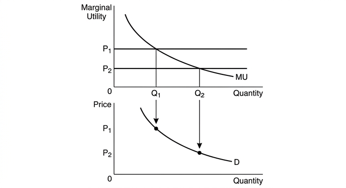
The diagram shows the MU curve sloping downward. At price P1, the consumer buys Q1 where MU = P1. When the price falls to P2, the consumer increases consumption to Q2 where MU = P2. The points (P1, Q1) and (P2, Q2) trace out the demand curve D. Thus, the theory provides a logical and intuitive explanation for the law of demand.
Limitations of marginal utility theory
Despite its elegance, marginal utility theory suffers from several weaknesses that prevent it from fully explaining the price–quantity link.
First, it assumes a rational consumer who can measure utility cardinally and make precise calculations. In reality, consumers have bounded rationality, are influenced by advertising and habits, and often make decisions based on imperfect information. Behavioural economics shows that choices are affected by framing, heuristics, and biases, which the theory ignores.
Second, the theory assumes the marginal utility of money is constant. This is unrealistic because the value of an additional dollar depends on a person's income and wealth. A dollar is worth more to a poor person than to a rich one, so the marginal utility of money changes with the level of spending.
Third, the theory relies on the ceteris paribus assumption that tastes, income, and the prices of other goods remain unchanged. In practice, these factors change frequently, and each change would require a recalculation of the demand schedule. The theory does not offer a dynamic framework to handle such changes.
Fourth, marginal utility theory does not distinguish between the income effect and the substitution effect of a price change. This omission means it cannot explain Giffen goods, where a rise in price leads to an increase in quantity demanded because the income effect outweighs the substitution effect. The theory would predict a downward-sloping demand curve for all goods, which is contradicted by the existence of Giffen goods.
Fifth, the theory is difficult to apply to one-off or durable goods, such as a house or a car, where consumption is not repeated in small units and marginal utility is not easily defined.
Evaluation
Marginal utility theory offers a clear and logical foundation for the law of demand. The concept of diminishing marginal utility is intuitively plausible and remains a cornerstone of microeconomics. However, the theory's assumptions are too restrictive to capture the full complexity of consumer behaviour. Modern indifference curve analysis, which uses ordinal utility and incorporates income and substitution effects, provides a more robust explanation of demand. It can account for Giffen goods and does not require the assumption of constant utility of money. Therefore, while marginal utility theory is a useful pedagogical tool, it cannot fully explain the link between price and quantity demanded.
Conclusion
Marginal utility theory cannot fully explain the link between a changing price and quantity demanded. Its assumptions of rational behaviour, constant utility of money, and ceteris paribus are unrealistic, and it fails to account for income and substitution effects, Giffen goods, and one-off purchases. Nonetheless, it remains a valuable starting point for understanding the inverse relationship and introduces key concepts that underpin more advanced theories of demand.
Marginal utility theory cannot fully explain the link between price and quantity demanded because its assumptions are too restrictive and it fails to account for income and substitution effects, Giffen goods, and one-off purchases; it offers only a partial explanation.
Background Concept
Marginal utility theory is a cardinal utility theory that attempts to explain consumer choice. Total utility (TU) is the total satisfaction from consuming a given quantity of a good. Marginal utility (MU) is the change in total utility from consuming one additional unit. The law of diminishing marginal utility states that as consumption increases, the marginal utility from each additional unit eventually falls. The equi-marginal principle states that a consumer maximises total utility when the marginal utility per dollar spent is equal across all goods: MUx/Px = MUy/Py = ... = MU of money (lambda). For a single good, if we assume the marginal utility of money is constant, then the consumer will consume until MU = P * lambda. If we normalise lambda = 1, then MU = P. Thus, the demand curve is essentially the marginal utility curve measured in money terms. As price falls, the consumer buys more until the diminishing MU falls to the new price. This generates a downward-sloping demand curve.
Understanding the Question
The question asks: "Evaluate whether marginal utility theory can fully explain the link between the changing price of a good and quantity demanded of that good." This requires you to first explain how marginal utility theory accounts for the inverse relationship between price and quantity demanded (the law of demand). Then, you must critically assess the theory's limitations and decide whether it provides a complete explanation. The command word "Evaluate" means you must present both sides (strengths and weaknesses) and reach a justified conclusion. The top band requires detailed knowledge, developed analysis, a diagram fully explained, and a reasoned evaluative conclusion.
Approach
- Begin by defining key terms: marginal utility, total utility, diminishing marginal utility, equi-marginal principle.
- Explain how the theory derives the demand curve: using the equi-marginal principle and the assumption of constant marginal utility of money, the consumer equates MU to price, leading to a downward-sloping demand curve. Include a diagram to illustrate this derivation.
- Present the limitations of the theory: unrealistic assumptions (rationality, constant MU of money, ceteris paribus), inability to distinguish income and substitution effects (hence cannot explain Giffen goods), and difficulty with one-off goods.
- Evaluate the overall explanatory power: weigh the strengths (logical foundation, intuitive appeal) against the weaknesses (restrictive assumptions, incompleteness).
- Conclude with a clear judgement: the theory cannot fully explain the link, but it offers a useful partial explanation.
Step-by-Step Reasoning
Step 1: Explanation of the theory
Define marginal utility and the law of diminishing marginal utility. Explain that a rational consumer aims to maximise total utility given their budget. The equi-marginal principle states that utility is maximised when the marginal utility per dollar is equal across all goods. For a single good, if we assume the marginal utility of money is constant, the condition simplifies to MU = P (if we set the MU of money = 1). This means the consumer will purchase units of the good until the marginal utility of the last unit equals its price. Because MU diminishes, a lower price means the consumer will purchase more units before MU falls to the new price. Thus, there is an inverse relationship between price and quantity demanded, which is the law of demand.
Step 2: Diagram
Draw a diagram with two panels. The upper panel has 'Marginal Utility' on the vertical axis and 'Quantity' on the horizontal axis. Draw a downward-sloping MU curve. At price P1, draw a horizontal line from the price axis to intersect MU at Q1. At a lower price P2, draw another horizontal line intersecting MU at a higher Q2. The lower panel has 'Price' on the vertical axis and 'Quantity' on the horizontal axis. Plot points (P1, Q1) and (P2, Q2) and draw a downward-sloping demand curve D through them. Arrows show the mapping. Explain that the demand curve is essentially the MU curve (with price on the vertical axis) because the consumer equates MU to price.
Step 3: Limitations
- Rational consumer assumption: The theory assumes consumers are perfectly rational and can measure utility cardinally. In reality, consumers have bounded rationality, are influenced by advertising, social norms, and cognitive biases. Behavioural economics shows that choices are often inconsistent with utility maximisation.
- Constant marginal utility of money: The theory assumes that the marginal utility of money is constant, meaning that the value of an additional dollar does not change as income changes. This is unrealistic; the marginal utility of money likely diminishes as income rises. This assumption is necessary for the simple MU = P condition, but it limits the theory's applicability.
- Ceteris paribus assumption: The theory assumes that tastes, income, and prices of other goods remain constant. In reality, these factors change, and the theory does not provide a way to analyse the effects of such changes without recalculating the entire demand schedule.
- Income and substitution effects: A price change has both a substitution effect (change in relative prices) and an income effect (change in real income). Marginal utility theory does not separate these effects. This means it cannot explain Giffen goods, where a rise in price leads to an increase in quantity demanded because the income effect (negative for a normal good) is so strong that it outweighs the substitution effect. The theory would predict a downward-sloping demand curve for all goods, which is contradicted by the existence of Giffen goods.
- One-off goods: The theory is designed for goods that are consumed in small, repeated units. For durable or one-off purchases (e.g., a house, a car), the concept of marginal utility over successive units is not straightforward, and the theory struggles to explain such purchases.
Step 4: Evaluation
Weigh the strengths against the weaknesses. The theory provides a clear, logical explanation for the law of demand and introduces the important concept of diminishing marginal utility. It is a useful pedagogical tool. However, its assumptions are too restrictive to capture real-world complexity. Modern demand theory, using indifference curves and budget lines, overcomes many of these limitations by using ordinal utility (no need for cardinal measurement) and by explicitly separating income and substitution effects. This theory can explain Giffen goods and does not require constant marginal utility of money. Therefore, while marginal utility theory offers a partial explanation, it cannot fully explain the link between price and quantity demanded.
Step 5: Conclusion
State clearly that marginal utility theory cannot fully explain the link. Justify this by summarising the key limitations and noting that more comprehensive theories exist. However, acknowledge that it remains a valuable starting point.
Key Takeaways
- Marginal utility theory explains the law of demand through diminishing marginal utility and the equi-marginal principle.
- The theory assumes rational behaviour, constant marginal utility of money, and ceteris paribus.
- These assumptions limit its explanatory power; it cannot account for income and substitution effects, Giffen goods, or one-off purchases.
- Modern indifference curve analysis provides a more complete explanation of demand.
- The question tests your ability to both explain a theory and critically evaluate its limitations.
Common Mistakes
- One-sided answer: Only explaining the theory without evaluating its limitations. This would score zero for evaluation (AO3).
- Omitting the diagram: The top band requires a diagram fully explained. Missing it caps the mark at Level 2.
- No conclusion: The top band requires a justified conclusion. A summary without a judgement is insufficient.
- Confusing marginal and total utility: Ensure you use the terms correctly.
- Overstating the theory's power: Claiming the theory fully explains demand without acknowledging limitations is incorrect.
- Understating the theory's contribution: Dismissing it as completely useless ignores its historical and pedagogical value.
Things to Be Careful About
- Diagram: Ensure the diagram is clearly labelled and explained in the text. Use correct axis labels and curve labels.
- Use of terminology: Use terms like 'diminishing marginal utility', 'equi-marginal principle', 'cardinal utility', 'ordinal utility' accurately.
- Address the question directly: The question asks about the link between changing price and quantity demanded. Keep the focus on that link.
- Evaluation: Make sure to evaluate, not just list limitations. Weigh the strengths and weaknesses.
- Conclusion: State a clear judgement and justify it. Avoid fence-sitting without a reasoned decision.
- Ceteris paribus: Explain why this assumption is problematic in the context of the theory.
- Giffen goods: Explain why they pose a problem for marginal utility theory.
Privatisation is often required by the International Monetary Fund (IMF) and the World Bank before they are prepared to offer support to countries requiring loans, grants, debt relief and debt cancellation programs.
Evaluate the view that privatisation will always improve the allocation of resources in a country.
Introduction
Privatisation is the transfer of ownership and control of state-owned enterprises (SOEs) to the private sector. Resource allocation refers to how an economy distributes its scarce resources among competing uses, judged by productive efficiency (producing at minimum average cost) and allocative efficiency (producing the mix of goods that consumers value most, where price equals marginal cost). This essay evaluates whether privatisation always improves resource allocation.
The case that privatisation improves allocation
Privatisation can improve resource allocation through several channels. First, private firms are driven by profit, which gives them a strong incentive to minimise costs and eliminate X-inefficiency – the slack that often exists in SOEs with no profit motive. This raises productive efficiency. Second, if privatisation is accompanied by deregulation and the breaking up of monopolies, competition increases. In a competitive market, firms must produce at the lowest possible cost and set price close to marginal cost, achieving allocative efficiency. Third, privatisation removes the burden of loss-making SOEs from the government budget, freeing funds for public goods like education and health, which can improve overall welfare. Fourth, private firms have better access to capital markets and can invest more efficiently than SOEs constrained by government borrowing limits. These arguments suggest that privatisation can move an economy closer to the efficient frontier.
The case against privatisation always improving allocation
However, privatisation does not guarantee improved allocation. A key counter-argument is the problem of natural monopoly. In industries such as water, electricity grids, and railways, the long-run average cost curve declines over the entire range of market demand, meaning a single firm can produce at lower cost than multiple firms. Breaking up such a natural monopoly to create competition would raise average costs and reduce productive efficiency. If the state monopoly is simply replaced by a private monopoly, the profit-maximising firm will restrict output and charge a price above marginal cost, creating a deadweight welfare loss and allocative inefficiency. Regulation can mitigate this, but regulators face information asymmetries and may be captured by the industry, leading to government failure. Moreover, private firms only consider private costs and benefits; they ignore negative externalities such as pollution. An SOE might be required to internalise external costs, whereas a private firm will not, worsening social welfare. Finally, privatisation can worsen equity: profitable SOEs sold cheaply transfer wealth to the wealthy, and job losses in restructured firms increase unemployment, imposing costs on the state through benefits. These factors can reduce overall welfare even if static efficiency improves.
Evaluation
The impact of privatisation on resource allocation depends critically on market structure and the regulatory framework. In competitive industries with low barriers to entry, privatisation is likely to improve both productive and allocative efficiency. In natural monopolies, privatisation without effective regulation can reduce welfare; with strong regulation (e.g., price caps, quality standards), it may still yield efficiency gains. The presence of externalities also matters: if the industry generates significant negative externalities, privatisation may worsen social allocation unless accompanied by corrective taxes or permits. Time period is relevant: short-run gains from cost-cutting may come at the expense of long-run investment if the private firm underinvests. The evidence from countries that have privatised is mixed: some saw improved efficiency (e.g., UK telecoms), while others experienced higher prices and reduced access (e.g., water in some developing countries).
Conclusion
Privatisation does not always improve resource allocation. Its success depends on the industry's market structure, the effectiveness of regulation, and the handling of externalities and equity. In competitive markets with proper regulation, privatisation can enhance efficiency; in natural monopolies or where externalities are significant, it may worsen allocation. Therefore, the view that privatisation will always improve allocation is not supported; a case-by-case assessment is required.
Privatisation does not always improve resource allocation; its effect depends on market structure, the presence of externalities, and the effectiveness of regulation.
Background Concept
Privatisation is the sale of state-owned enterprises (SOEs) to private investors. Resource allocation refers to how an economy uses its scarce resources to produce goods and services. Two key efficiency concepts are used to judge allocation:
- Productive efficiency: producing at the lowest possible average cost (on the LRAC curve).
- Allocative efficiency: producing the mix of goods that consumers value most, achieved when price equals marginal cost (P = MC).
In a perfectly competitive market, both efficiencies are achieved in the long run. However, real markets often fail due to monopoly, externalities, or public goods. Privatisation is often advocated as a way to improve efficiency by introducing profit incentives and competition. But the claim that it always improves allocation is an absolute statement that must be tested against economic theory and evidence.
Understanding the Question
The question asks you to evaluate the statement: "Privatisation will always improve the allocation of resources in a country." The command word "Evaluate" requires you to present both sides of the argument and reach a justified conclusion. The word "always" makes the statement absolute, so the counter-case is essential: you must show conditions under which privatisation might worsen allocation. The question is from the A-Level Paper 4 (20 marks, levels-based). The top band requires detailed knowledge, developed analysis, accurate use of diagrams, and a justified conclusion.
Approach
- Define key terms: privatisation, resource allocation (productive and allocative efficiency).
- Present the case for privatisation: profit motive reduces X-inefficiency, competition improves efficiency, fiscal benefits, access to capital.
- Present the case against: natural monopoly leads to private monopoly inefficiency, externalities ignored, equity concerns, job losses.
- Evaluate: weigh the arguments on criteria such as market structure, regulation, externalities, and time period.
- Conclude: state that privatisation does not always improve allocation; it depends on conditions.
- Include a diagram: a natural monopoly diagram to illustrate the inefficiency of private monopoly and the role of regulation.
Step-by-Step Reasoning
Step 1: Define privatisation and efficiency.
Start by explaining that privatisation transfers ownership from the state to private hands. Resource allocation is assessed by productive and allocative efficiency. This sets the framework.
Step 2: Build the case that privatisation improves allocation.
- Profit motive: Private firms aim to maximise profit, so they cut waste (X-inefficiency). SOEs often have soft budget constraints and no incentive to minimise costs.
- Competition: If privatisation breaks up a monopoly and lowers barriers to entry, firms compete. In a competitive market, firms must produce at minimum AC (productive efficiency) and set P = MC (allocative efficiency).
- Fiscal benefits: Selling SOEs raises revenue for the government, which can reduce debt or fund public services. Loss-making SOEs no longer drain the budget.
- Access to capital: Private firms can raise funds from capital markets, allowing efficient investment without government borrowing constraints.
Step 3: Build the case against privatisation always improving allocation.
- Natural monopoly: In industries with declining LRAC (e.g., water, railways), a single firm is most efficient. Breaking it up raises costs. If the privatised firm remains a monopoly, it will produce where MR = MC, charging a price above MC, causing a deadweight loss. This is allocatively inefficient.
- Regulation challenges: Even with a regulator, information asymmetry and regulatory capture can lead to poor outcomes. The need for regulation itself suggests privatisation does not automatically improve allocation.
- Externalities: Private firms ignore external costs (e.g., pollution). An SOE might be required to consider social costs, but a private firm will not unless forced by taxes or permits. This can worsen social welfare.
- Equity: Profitable SOEs sold cheaply transfer wealth to the rich. Job losses increase unemployment benefits, raising government spending. These distributional effects can reduce overall welfare even if static efficiency improves.
Step 4: Evaluate the arguments.
- Market structure: In competitive industries, privatisation likely improves efficiency. In natural monopolies, it may worsen it unless regulation is strong.
- Regulation: Effective regulation (price caps, quality standards) can mimic competitive outcomes, but it is costly and imperfect. The success of privatisation often hinges on the quality of regulation.
- Externalities: If the industry has significant negative externalities, privatisation without corrective policies can reduce social welfare. If externalities are small, the efficiency gains may dominate.
- Time period: Short-run cost-cutting may boost profits but reduce long-run investment (e.g., underinvestment in infrastructure). Dynamic efficiency may suffer.
- Evidence: The UK's privatisation of telecoms (BT) improved efficiency and lowered prices, but water privatisation led to price rises and underinvestment. Developing countries often saw mixed results.
Step 5: Diagram explanation.
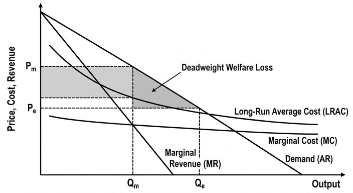
The diagram shows a natural monopoly. The LRAC curve slopes downward over the relevant range, indicating economies of scale. The demand curve (AR) is downward sloping. The profit-maximising private monopolist produces where MR = MC, at output Qm and price Pm. This is allocatively inefficient because Pm > MC. The allocatively efficient output is where P = MC, at Qe and price Pe. However, at Qe, the firm makes a loss because P < LRAC. Therefore, a natural monopoly cannot be forced to produce at P = MC without a subsidy. Regulation often sets price at P = LRAC (average cost pricing) to allow a normal profit, achieving a second-best outcome. The diagram illustrates that privatisation of a natural monopoly without regulation leads to allocative inefficiency, and even with regulation, the outcome is not first-best.
Step 6: Conclusion.
The conclusion must be justified. State that privatisation does not always improve allocation; it depends on market structure, regulation, and externalities. In competitive markets with good regulation, it can improve efficiency; in natural monopolies or where externalities are significant, it may worsen allocation. Therefore, the absolute claim is false.
Key Takeaways
- Privatisation can improve efficiency through profit incentives and competition, but it is not a panacea.
- The outcome depends on market structure: competitive markets benefit, natural monopolies require careful regulation.
- Externalities and equity considerations can offset efficiency gains.
- A diagram of natural monopoly is a powerful tool to illustrate the counter-case.
- Always address absolute claims by showing conditions where they fail.
Common Mistakes
- One-sided answer: Only arguing that privatisation is good or bad. The question requires both sides; a one-sided response scores zero for evaluation.
- No conclusion or vague conclusion: The top band requires a justified conclusion that addresses the specific question. Simply summarising both sides is not enough.
- Missing diagram: The indicative content and level descriptors expect a diagram. Omitting it caps the mark at Level 2.
- Unexplained diagram: Drawing a diagram without explaining it in the text loses marks. The diagram must be integrated into the analysis.
- Confusing privatisation with deregulation: Privatisation is about ownership; deregulation is about removing rules. They often go together but are distinct.
- Ignoring the word 'always': The absolute nature of the statement is the key to the evaluation. The counter-case must directly challenge the 'always'.
Things to Be Careful About
- Label all axes and curves on the diagram clearly (price, quantity, MC, MR, AR, LRAC).
- Use economic terminology precisely: X-inefficiency, deadweight loss, natural monopoly, allocative efficiency.
- Develop chains of reasoning: explain why each effect occurs, not just state it.
- In the evaluation, use criteria like market structure, time period, and externalities to weigh the arguments.
- Ensure the conclusion is a judgement, not a restatement. Say under what conditions privatisation improves allocation and when it does not.
The table below contains some key economic data for Mexico in 2020.
| Gross National Income (GNI) | 18.5 billion pesos |
|---|---|
| nominal wages | +2.8% |
| disposable income | +1.2% |
| unemployment rate | 4.2% |
| population growth rate | 1.1% |
| inflation rate | 3.4% |
Source: knoema.com
Evaluate the use of these statistics in assessing the standard of living in Mexico in 2020.
Introduction
Standard of living (SoL) encompasses both material wellbeing (income, consumption) and non-material aspects (health, education, environment). The table provides five statistics for Mexico in 2020. This essay evaluates their usefulness in assessing SoL, considering what they reveal and what they omit.
Analysis of the statistics
Gross National Income (GNI) of 18.5 billion pesos is a nominal, aggregate measure. It does not account for population size or inflation. Without population data, we cannot calculate GNI per capita, which is a better indicator of average material living standards. The nominal value also ignores price changes; real GNI would be more meaningful.
Nominal wages +2.8% and inflation 3.4%: The real wage growth is approximately 2.8% - 3.4% = -0.6%, i.e. a fall in real wages. This suggests that the purchasing power of workers declined, negatively affecting material SoL. However, this is an average; distribution matters.
Disposable income +1.2%: This is also nominal. Real disposable income fell by about 3.4% - 1.2%? Actually real change = nominal change - inflation = 1.2% - 3.4% = -2.2%. This indicates households had less real income to spend, reducing material wellbeing. But again, averages obscure inequality.
Unemployment rate 4.2%: A relatively low unemployment rate suggests that most people willing to work are employed, which supports material SoL. However, it does not capture underemployment, labour force participation, or job quality (e.g. informal sector).
Population growth 1.1%: This is relevant because if GNI is growing slower than population, GNI per capita falls. The table does not provide GNI growth, so we cannot assess this. Population growth alone tells little about SoL; it may strain public services.
Evaluation
The statistics are limited in several ways. First, they are nominal and aggregate, so real per capita values are unknown. Second, they only capture material aspects; non-material dimensions like health, education, and environmental quality are absent. Third, the data are for a single year (2020), so trends cannot be identified. Fourth, the statistics do not show distribution – inequality may be high even if averages are moderate. Fifth, the unemployment rate may understate the problem if discouraged workers exist. Sixth, the data do not account for purchasing power parity (PPP); Mexico's price level may differ from other countries, so comparisons are difficult.
To improve assessment, we would need real GNI per capita, the Gini coefficient, the Human Development Index (HDI) which includes life expectancy and education, and measures of deprivation like the Multidimensional Poverty Index (MPI). The table provides a starting point but is insufficient for a comprehensive evaluation.
Conclusion
While the statistics offer some insight into material aspects of standard of living in Mexico in 2020, they are severely limited by being nominal, aggregate, and lacking non-material data. The fall in real wages and real disposable income indicate a decline in material wellbeing, but a full assessment requires per capita real measures and composite indicators like HDI. Therefore, the statistics are useful only as a partial and preliminary guide; they are insufficient for a robust evaluation of standard of living.
The statistics provide a partial picture of material living standards, but their limitations (nominal values, lack of per capita data, no non-material indicators) mean they are insufficient for a comprehensive assessment; a composite indicator like HDI would be more useful.
Background Concept
Standard of living (SoL) is a broad concept encompassing the material wellbeing (income, consumption, wealth) and non-material quality of life (health, education, political freedom, environment). Economists often use monetary indicators like GDP per capita (or GNI per capita) as proxies, but these have well-known limitations: they ignore distribution, non-market activities, externalities, and leisure. Non-monetary indicators such as life expectancy, literacy rates, and composite indices like the Human Development Index (HDI) attempt to capture a fuller picture. The HDI combines income, education, and health. Other measures include the Measure of Economic Welfare (MEW) and the Multidimensional Poverty Index (MPI).
Understanding the Question
The question presents a table of five economic statistics for Mexico in 2020: nominal GNI, percentage changes in nominal wages and disposable income, unemployment rate, population growth rate, and inflation rate. It asks you to evaluate the use of these statistics in assessing the standard of living in Mexico. This is a 20-mark essay, levels-based, with AO1+AO2 out of 14 and AO3 out of 6. The top band requires detailed knowledge of the concepts, a fully developed analysis of each statistic's relevance, and then a justified evaluative conclusion that addresses the specific question. The command word 'Evaluate' means you must discuss both strengths and weaknesses and reach a judgement.
Approach
Start by defining standard of living and distinguishing material from non-material aspects. Then systematically analyse each statistic: what it tells us about SoL, what it does not tell us, and how it interacts with other data. For example, compare nominal wage growth with inflation to deduce real wage change. Discuss the limitations of aggregate, nominal data without per capita or real adjustment. Then evaluate the overall usefulness: the data provide some information on material conditions but are incomplete. Finally, suggest what additional data would improve the assessment (e.g., real GNI per capita, HDI, Gini coefficient). The conclusion should state that the statistics are only partially useful, and a comprehensive assessment requires more.
Step-by-Step Reasoning
-
Define SoL: Material SoL refers to the ability to consume goods and services; non-material includes health, education, environment. The table gives only monetary and labour market data.
-
GNI 18.5 billion pesos: This is a nominal, aggregate figure. To assess average material wellbeing, we need GNI per capita (divide by population). But population is not given in absolute terms, only growth rate. Without base year population, we cannot compute per capita. Also, nominal means not adjusted for inflation; real GNI would require a price deflator. The table does not provide the base year, so we cannot determine if GNI is high or low in real terms.
-
Nominal wages +2.8% and inflation 3.4%: A simple calculation: real wage change ≈ nominal wage change - inflation rate = 2.8% - 3.4% = -0.6%. So real wages fell, implying workers' purchasing power decreased. This is a negative impact on material SoL. However, this is an average; some workers may have experienced different changes. Also, the wage data might be for formal sector only, ignoring informal workers.
-
Disposable income +1.2%: Similarly, real disposable income change ≈ 1.2% - 3.4% = -2.2%. This is a larger fall, indicating households had less real income after taxes and transfers. This reduces material wellbeing. But again, distribution matters.
-
Unemployment rate 4.2%: A low unemployment rate is generally positive for SoL because most people who want jobs have them. However, it does not capture underemployment (people working part-time who want full-time), or the quality of jobs (low wages, insecure work). Also, the labour force participation rate is not given; if participation is low, a low unemployment rate may hide discouraged workers. In Mexico, the informal sector is large, so the official unemployment rate may understate the problem.
-
Population growth 1.1%: This is a rate. To assess its impact on SoL, we need to compare it with GNI growth. If GNI grows slower than population, GNI per capita falls, reducing material SoL. The table does not give GNI growth, so we cannot evaluate that. Population growth also affects non-material SoL through pressure on infrastructure, education, and health services.
-
Evaluation - Strengths: The data are relatively easy to obtain and provide a snapshot of some key economic variables. The combination of wage and inflation data allows a simple calculation of real income change, which is a useful indicator. The unemployment rate gives a quick read of labour market conditions.
-
Evaluation - Weaknesses: The data are nominal, aggregate, and for a single year. They do not allow calculation of real per capita measures. They ignore distribution (inequality), non-material aspects, and environmental sustainability. The unemployment rate is a narrow measure. The table does not include data on health, education, or housing. Also, the data are for 2020, a year affected by the COVID-19 pandemic, which may distort normal patterns, but the question does not mention that explicitly.
-
Conclusion: The statistics are only partially useful. They give some indication of material trends (falling real incomes) but are insufficient for a comprehensive assessment. To properly evaluate SoL, we need real GNI per capita, the Gini coefficient, the HDI, and possibly the MPI. Therefore, while these statistics are a starting point, they are not adequate for a robust evaluation.
Key Takeaways
- Standard of living is multidimensional; monetary indicators are only part of the picture.
- Nominal data must be adjusted for inflation and population to be meaningful.
- Aggregate data hide distributional issues.
- Composite indicators like HDI provide a more holistic assessment.
- When evaluating the usefulness of statistics, consider what they measure, what they omit, and how they can be improved.
Common Mistakes
- Failing to adjust nominal values for inflation or population. Many students simply list the statistics without performing the real wage calculation.
- Treating the unemployment rate as a comprehensive measure of labour market health without acknowledging underemployment or informal sector.
- Ignoring the need for growth rates in GNI to compare with population growth.
- Providing a one-sided evaluation (only strengths or only weaknesses) without a balanced judgement. The command word 'Evaluate' requires both sides and a conclusion.
- Ending without a justified conclusion, or with a vague conclusion like 'it depends'.
- Not using economic terminology such as 'real', 'nominal', 'per capita', 'purchasing power', 'composite indicator'.
Things to Be Careful About
- The question says 'these statistics' – do not add statistics that are not in the table, but you can suggest additional ones for evaluation.
- Be precise with calculations: real change = nominal change - inflation rate. Show the working.
- Distinguish between material and non-material SoL explicitly.
- The conclusion must directly answer the question: evaluate the use of these statistics. State whether they are useful or not, and to what extent.
- Use the extract's data: you must mention the specific figures (e.g., 18.5 billion pesos, 2.8%, 3.4%, etc.) to ground your analysis.
Between 2010 and 2020, very low interest rates encouraged low-income countries to borrow money from foreign investors and governments to finance long-term economic growth.
Evaluate this approach to promoting long-term economic growth.
Introduction
Long-term economic growth refers to an increase in an economy’s productive capacity, measured by the growth of potential GDP over time. Low-income countries often face a domestic savings gap, which limits their ability to finance investment in physical capital, infrastructure, and technology. Foreign borrowing from governments, international agencies, and private investors can provide the necessary funds to close this gap and stimulate growth.
The case for foreign borrowing
Foreign capital inflows allow low-income countries to invest in projects that raise both aggregate demand and aggregate supply. In the short run, spending on construction and equipment increases aggregate demand (AD), boosting output and employment. In the long run, the accumulation of capital, together with possible technology transfer from multinational corporations, shifts the long-run aggregate supply (LRAS) curve to the right, expanding potential output.
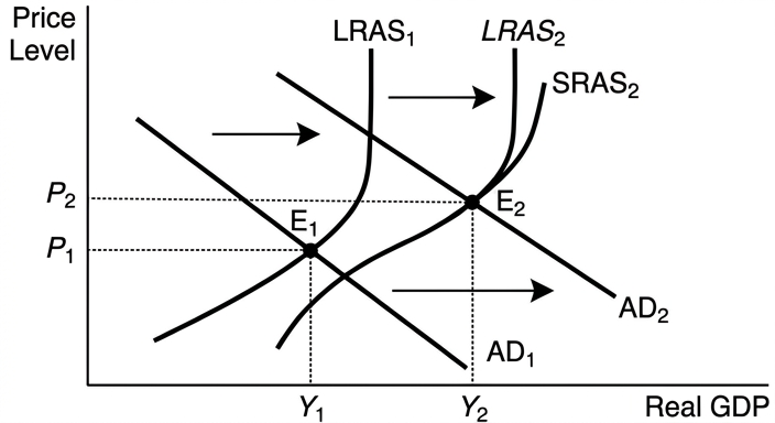
The diagram shows an outward shift of both AD and LRAS, leading to higher real GDP in the long run. For example, China’s Belt and Road Initiative financed infrastructure in numerous low-income countries, which helped raise their productive capacity. Similarly, loans from the World Bank have supported education and health projects that improve human capital. With interest rates at historic lows between 2010 and 2020, the cost of borrowing was relatively cheap, making such investment more attractive. If the marginal efficiency of capital (MEC) exceeds the interest rate, the investment is profitable and should yield a positive return.
The case against foreign borrowing
Despite the potential benefits, foreign borrowing carries significant risks. First, the borrowed funds must be repaid with interest. If global interest rates rise, as they did after 2020, the cost of servicing debt increases, diverting government revenue from other spending and worsening the current account of the balance of payments. Many low-income countries borrow in foreign currency, so a depreciation of their exchange rate raises the local currency cost of debt. This can trigger a debt crisis, as seen in Zambia and Sri Lanka. Second, the quality of investment projects is critical. Borrowing may finance “vanity projects” (e.g., prestige roads or buildings) that have little economic return, failing to generate the output needed to repay loans. Third, if the borrowed funds are used to import capital goods from the lending country, the multiplier effect is reduced, and there may be a negative impact on the domestic trade balance. Fourth, reliance on foreign borrowing can create macroeconomic vulnerability; countries become exposed to shifts in global investor sentiment, commodity price fluctuations, and policy changes in creditor nations.
Evaluation
The effectiveness of foreign borrowing as a growth strategy depends on several factors. The most important is the productivity of the investments: if projects have high social and private returns, the resulting growth will generate the resources to service debt. The terms of borrowing matter: concessional loans with low interest and long maturities are more sustainable than commercial borrowing. The institutional capacity of the borrowing country to select, implement, and monitor projects is crucial; countries with strong governance and low corruption fare better. Additionally, the macroeconomic environment — including a stable exchange rate, diversified exports, and prudent fiscal policy — reduces vulnerability. In the case of countries like Botswana, foreign borrowing combined with sound management led to sustained growth, whereas in others it exacerbated indebtedness and instability.
Conclusion
Foreign borrowing can be an effective tool to promote long-term economic growth in low-income countries, particularly when used to finance high-return investment in infrastructure and human capital. However, the approach is not without risks — rising global interest rates, debt sustainability problems, and poor project selection can undermine its benefits. A justified conclusion is that borrowing is most likely to succeed when accompanied by strong institutions, careful project appraisal, and a diversified economic base that reduces external vulnerability. On balance, while the approach can work, it requires careful management and is not a guaranteed path to growth.
Foreign borrowing can promote long-term growth if used for productive investment and managed prudently, but success depends on institutional quality and global economic conditions; it is not a guaranteed strategy.
Background Concept
Long-term economic growth means an increase in the economy's potential output, shown by an outward shift of the production possibility curve or the long-run aggregate supply curve. Growth requires investment in physical capital (machinery, infrastructure), human capital (education, health), and technology. Low-income countries typically have low per capita incomes, which limit domestic saving. Without adequate saving, investment is constrained. Foreign borrowing — from governments, international organisations like the World Bank, or private lenders — can fill this “savings gap”. The borrowed funds are used to finance investment projects. The marginal efficiency of capital (MEC) is the expected rate of return on investment; if it exceeds the interest rate, the investment is worthwhile. The AD/AS model shows both short-run demand effects and long-run supply effects.
Understanding the Question
The question asks you to evaluate the approach of low-interest-rate borrowing by low-income countries to finance long-term growth. The command word “Evaluate” requires a two-sided analysis: you must present arguments for and against, then weigh them, and reach a justified conclusion. The specific context is the period 2010–2020 when interest rates were very low globally, encouraging borrowing. The question expects you to consider both the potential benefits (cheap loans funding infrastructure, technology transfer, etc.) and the risks (debt sustainability, rising interest rates later, project misuse, balance of payments problems). The top band demands a detailed chain of reasoning, use of analytical tools such as the AD/AS diagram, fully developed explanations, and a justified conclusion that directly addresses the question.
Approach
The essay will follow a structured four-part approach: (1) Explain the rationale for foreign borrowing and how it can lead to long-term growth, using the AD/AS diagram. (2) Present the counter-arguments, highlighting the risks and potential downsides. (3) Evaluate the two sides by identifying the conditions under which borrowing is more or less effective. (4) Conclude with a justified judgement that answers the question directly. The AD/AS diagram will illustrate the dual short-run and long-run effects. The evaluation will focus on the quality of projects, terms of borrowing, institutional strength, and external economic conditions.
Step-by-Step Reasoning
Step 1: Define long-term growth – It is sustained increase in potential GDP, driven by increases in factors of production and productivity. Low-income countries need capital formation.
Step 2: Explain the savings gap – With low incomes, saving is low, so domestic funds for investment are scarce. Foreign borrowing provides external funds.
Step 3: Build the positive chain – Borrowed money is spent on investment goods (e.g., building roads, ports, factories). This increases aggregate demand in the short run (AD shifts right), raising real GDP and employment. Over time, the new capital increases the productive capacity of the economy: LRAS shifts right. If productivity also improves through technology transfer (e.g., from MNCs), growth can be even stronger. The diagram labels: initial equilibrium at E1 (P1, Y1); AD shifts to AD2; LRAS shifts to LRAS2; new long-run equilibrium at E2 (P2, Y2) with higher Y. The low interest rates from 2010–2020 made borrowing cheap: the MEC could exceed the low interest rate, making many investments profitable.
Step 4: Present the risks – First, interest rate risk: if global rates rise, debt servicing becomes more expensive. Since many low-income countries borrow in US dollars, any depreciation of their currency increases the domestic cost of debt. Second, the risk of unproductive investment: governments may waste borrowed money on prestige projects with low returns, leaving the country with debt but no growth. Third, the import leakage: if borrowed funds are used to buy capital goods from abroad, the domestic multiplier is lower, and the current account deteriorates. Fourth, macroeconomic vulnerability: heavy reliance on foreign capital makes the economy sensitive to changes in investor confidence, commodity prices, and creditor policies. Examples of debt crises (Zambia, Sri Lanka) illustrate these points.
Step 5: Evaluate – The central criterion is the productivity of investment. If projects yield high social and private returns, growth will help repay debt. The terms of borrowing matter: concessional loans (low interest, long grace periods) are safer than commercial debt. Strong institutions (rule of law, low corruption, effective project management) improve outcomes. A diversified economy and stable macro policies reduce vulnerability. When these conditions are met, foreign borrowing can be successful. When they are absent, borrowing leads to crisis.
Step 6: Conclude – The approach can be effective but is not universally so. It works best when borrowing is directed at high-return projects, the terms are favourable, and the country has good governance. Therefore, the answer should state that it is a conditional yes: potentially beneficial but with significant risks that require careful management.
Key Takeaways
- Long-term growth requires investment; foreign borrowing can finance that investment when domestic savings are insufficient.
- The AD/AS model helps analyse both short-run demand effects and long-run supply effects.
- Evaluation of policies must consider multiple factors: productivity, terms, institutions, external environment.
- A justified conclusion weighs conditions and gives a nuanced verdict.
- This question tests the ability to connect micro-finance concepts (savings, investment, interest rates) with macro models (AD/AS) and development economics (debt sustainability).
Common Mistakes
- Writing a one-sided answer that only lists benefits or only drawbacks – loses all AO3 marks.
- Not using a diagram or using it without explaining it (e.g., just drawing shifts without labels or without discussing in text) – prevents top band for AO1/AO2.
- Failing to provide a clear conclusion or giving a vague “it depends” without specifying conditions – loses marks for evaluation.
- Describing rather than analysing: for example, just saying “borrowing is bad because of debt” without explaining the chain of causation from rising interest rates to debt crisis.
- Ignoring the specific context of low interest rates between 2010 and 2020 – the question expects you to consider that low rates were an incentive and that rates later rose.
- Providing too many shallow points instead of developing a few in depth.
- Not using real-world examples or evidence from the extract (though no extract here, but general examples help).
Things to Be Careful About
- Label the AD/AS diagram clearly: axes (price level, real GDP), curves (AD1, AD2, LRAS1, LRAS2, SRAS), equilibrium points.
- Explain the diagram in the text: state which curve shifts and why, and what happens to output and price level.
- Use correct terminology: “long-run aggregate supply”, “potential output”, “savings gap”, “marginal efficiency of capital”, “debt servicing”, “current account deficit”.
- Ensure the conclusion is justified, not a summary. The conclusion should directly answer the question: is this approach effective? Under what conditions?
- Avoid overgeneralising: not all borrowing is bad; not all low-income countries are the same. Distinguish between concessional and commercial borrowing, and between productive and unproductive projects.
- Watch for sign errors: rising interest rates increase the cost of borrowing, not decrease.
- Consider the time frame: short-run AD effects vs. long-run supply effects; the low interest rate period was temporary.
- Keep the essay organised: use clear paragraphs and logical progression from one argument to the next.