Economics 9708/41 — October/November 2024
Cambridge A-Level · A Level Data Response and Essays · worked solutions for every part, with the mark scheme
Topics Economic Growth and Sustainability · The Multiplier and National Income Determination · Exchange Rate Systems · Economic Development and Living Standards · Externalities, Social Costs and Benefits · Efficiency and Market Failure · +6 more
The economic impact of extracting natural resources
Many low-income countries have high unemployment and large deposits of unused natural resources. In 2007, Ghana discovered a new offshore oil field and extraction started in 2010. The discovery and extraction of such natural resources can create new jobs, that increase incomes and consequently gross national income (GNI). The additional income will lead to an increase in spending on both domestic and imported goods and services, creating further employment in other sectors through the multiplier effect.
However, the extraction of oil may 'crowd out' other sectors of the economy. Workers might move, for example from agriculture and manufacturing to the mining sector due to higher wages. Also, the prices of houses, land and locally produced goods may increase. This could increase the cost of living and discourage businesses from operating in the affected region.
The export of oil from Ghana causes an inflow of United States dollars (US$), increasing the exchange rate of Ghana's currency, the cedi. This appreciation reduces the competitiveness of Ghana's agricultural and manufactured goods, leading to an increased demand for imports. This loss of competitiveness is referred to as the 'Dutch disease', reflecting the experience of the Netherlands following the exploitation of their natural gas reserves.
Oil provides the Ghanaian government with revenue from the tax on each barrel of oil produced. This revenue can be used to provide transfer payments and goods and services such as roads, health facilities, and public water supply. These can benefit both households and businesses. Alternatively, the presence of such revenues can create corruption and conflict as political groups compete for them.
Between 2011 and 2018 agricultural products and food as a share of Ghana's exports have decreased, as shown in Fig. 1.1.
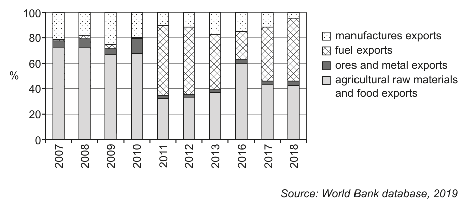
Fig. 1.1: Structure of exports of goods from Ghana 2007 to 2018
Source: World Bank database, 2019
The extraction of natural resources has also affected Ghana's economic performance, as shown in Table 1.1.
Table 1.1: Selected economic data for Ghana, 2007 and 2019
| 2007 | 2019 | |
|---|---|---|
| Human Development Index (HDI) | 0.55 | 0.61 |
| GNI per capita (US$) ppp | 2478 | 5484 |
| exchange rate (cedi per US$) | 1.06 | 0.17 |
With the aid of a diagram, explain the effect of natural resource development on the potential growth of Ghana.
Answer
Natural resource development increases the potential output of Ghana by expanding the economy's productive capacity. (1)
A production possibility curve (PPC) illustrates the maximum possible output of two goods an economy can produce with its current resources and technology. (1)
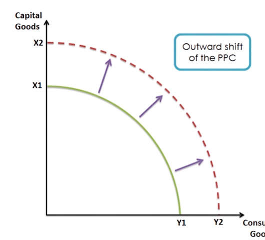
The diagram has 'Capital Goods' on the vertical axis and 'Consumer Goods' on the horizontal axis. The initial concave PPC runs between points X1 and Y1. The outward shift to the dashed outer PPC between X2 and Y2 represents the increase in potential output from the discovery and extraction of oil, which adds to Ghana's available factors of production. (1)
This outward shift means Ghana can now produce more of both capital and consumer goods than before, reflecting higher potential economic growth. (1)
Natural resource development increases Ghana's potential economic growth, illustrated by an outward shift of the production possibility curve (PPC).
Background Concept
Potential economic growth refers to an expansion in an economy's maximum sustainable output, determined by the quantity and quality of its factors of production (land, labour, capital, enterprise) and the state of its technology. Unlike actual growth, which is the change in real output over time, potential growth represents an outward shift in the economy's productive capacity. The production possibility curve (PPC) is a key model used to illustrate potential growth: it shows the maximum combinations of two goods an economy can produce when all resources are fully and efficiently employed. An outward shift of the PPC indicates an increase in potential output, caused by an increase in the quantity or quality of factors of production, or technological progress.
Understanding the Question
This question asks you to explain, with the aid of a diagram, how the development of natural resources (oil extraction in Ghana) affects the country's potential economic growth. The extract provides context: Ghana discovered oil in 2007 and began extraction in 2010, adding a new valuable factor of production (oil reserves) to its economy. The command word "explain" requires you to build a clear causal chain linking natural resource development to higher potential output, and to include a correctly labelled diagram to illustrate this relationship. The 4-mark tariff means you need to cover four distinct creditable points: a statement that potential growth increases, the relevant diagram shift, correct axis and curve labels, and an explanation of what the shift represents.
Approach
To answer this question, first define potential growth and state that natural resource development will increase it. Then draw a PPC (the most appropriate diagram for potential growth, as noted in the mark scheme) with correct labels: capital goods on the vertical axis, consumer goods on the horizontal axis. Show an outward shift of the PPC, and explain that this shift represents the increase in Ghana's productive capacity from the addition of oil reserves to its factor base. Ensure every part of the diagram is labelled, as unlabelled axes or curves lose marks.
Step-by-Step Reasoning
- First, state the core link: the discovery and extraction of oil adds a new valuable natural resource to Ghana's factor of production base. This increases the economy's maximum possible output, so potential economic growth increases. (1 mark)
- The PPC is the standard model for illustrating potential output. Draw the PPC with the vertical axis labelled "Capital Goods" and the horizontal axis labelled "Consumer Goods". The initial PPC is a concave curve showing the maximum output combinations before oil extraction. (1 mark for axes and initial curve)
- Draw a second, outer dashed PPC to represent the higher potential output after oil extraction. Add arrows pointing from the initial PPC to the outer PPC to show the direction of the shift. Label the outer PPC or add a text box stating "Outward shift of the PPC". (1 mark for the shift and labels)
- Explain the shift: the outward shift of the PPC shows that Ghana can now produce more of both capital and consumer goods than before, as the oil reserves add to the total available resources. This is an increase in potential growth, as the economy's productive capacity has expanded. (1 mark for explanation of the shift)
Key Takeaways
- Potential growth is an increase in an economy's maximum sustainable output, shown by an outward shift of the PPC or LRAS curve.
- An increase in the quantity or quality of factors of production (such as the discovery of oil reserves) causes the PPC to shift outward.
- Diagrams for potential growth must have correctly labelled axes and curves, and the direction of the shift must be clearly marked.
Common Mistakes
- Drawing a shift along the PPC instead of an outward shift: a movement along the PPC represents a reallocation of resources, not an increase in potential output.
- Forgetting to label the axes or curves: unlabelled diagrams lose marks, even if the shift is correct.
- Confusing potential growth with actual growth: potential growth is about the economy's capacity, not the actual change in output over time.
- Using an AD/AS diagram incorrectly: while LRAS can also show potential growth, the PPC is more appropriate for illustrating the effect of new factor resources, and the mark scheme explicitly accepts PPC.
Things to Be Careful About
- Ensure the PPC is drawn as a concave curve (bowed out from the origin), as this reflects increasing opportunity cost, which is a standard feature of the model.
- Clearly mark the direction of the shift with arrows, so the examiner can see the change at a glance.
- Explain the diagram in the prose, linking the shift to the specific context of Ghana's oil discovery, rather than just drawing the diagram without commentary.
Explain how the extraction of natural resources in Ghana will 'create further employment in other sectors through the multiplier effect'.
Answer
The multiplier is the total increase in national income (or output) that results from an initial injection of spending into the circular flow of income. (1)
The extraction of oil in Ghana creates new jobs in the mining sector, generating new incomes for workers. (1) These workers spend a proportion of their additional income on goods and services, creating further rounds of spending, income and employment in other sectors of the economy (such as retail, transport and services). (1) This successive process of spending and income generation is the multiplier effect, leading to higher total employment than just the jobs created directly in the oil sector. (1)
The multiplier effect means the initial injection of spending from oil extraction creates successive rounds of spending and income, generating additional employment in other sectors beyond the direct jobs in the oil industry.
Background Concept
The multiplier effect is a core concept in national income determination. It describes the process by which an initial injection of spending into the circular flow of income leads to a total increase in national income that is larger than the initial injection. This happens because when someone receives additional income, they spend a proportion of it (the marginal propensity to consume, MPC), creating income for someone else, who in turn spends a proportion of their new income, and so on. The size of the multiplier depends on the marginal propensities to consume, save, tax and import: the more leakages (savings, taxes, imports) from the circular flow, the smaller the multiplier. The multiplier process explains why an initial increase in investment, government spending or exports can have a larger overall impact on national income and employment than the initial spending alone.
Understanding the Question
This question asks you to explain how oil extraction in Ghana creates further employment in other sectors via the multiplier effect. The extract states that oil extraction creates new jobs and increases incomes, which then lead to more spending and employment in other sectors. The 4-mark tariff splits into 2 marks for knowledge and understanding of the multiplier, and 2 marks for applying this concept to the Ghana case study. You need to first define the multiplier clearly, then build a causal chain linking the initial injection from oil extraction to successive rounds of spending and employment creation in other sectors.
Approach
Start by defining the multiplier: the total increase in national income/output from an initial injection into the circular flow of income. Then apply this to Ghana's context: the initial injection is the spending and income generated by the oil extraction sector (new jobs, wages, investment in oil infrastructure). Explain that the workers and firms in the oil sector will spend their additional income on goods and services from other sectors (retail, transport, hospitality, etc.), creating new income for people in those sectors, who then spend their income, creating further rounds of spending and employment. Emphasise that this process leads to employment beyond just the direct jobs in the oil sector.
Step-by-Step Reasoning
- First, demonstrate knowledge of the multiplier: define it as the total increase in national income (or output) that results from an initial injection of spending into the circular flow of income. (1 mark for definition)
- Note that the initial injection in this case is the economic activity generated by oil extraction: new jobs in the mining sector, wages paid to oil workers, and investment in oil-related infrastructure. (1 mark for identifying the initial injection in the Ghana context)
- Explain the first round of the multiplier: oil workers and firms will spend a proportion of their additional income on goods and services from other sectors of the economy, such as food, housing, transport and retail. This spending creates new income for workers and firms in these sectors. (1 mark for first round of spending)
- Explain the subsequent rounds: the people who receive this new income will in turn spend a proportion of it on other goods and services, creating further rounds of income and spending. Each round creates additional employment in the sectors receiving the spending, so total employment across the economy is higher than just the direct jobs created in the oil sector. (1 mark for explaining the full multiplier process and employment effect)
Key Takeaways
- The multiplier effect describes how an initial injection of spending leads to a total increase in national income larger than the initial injection, via successive rounds of spending and income generation.
- The size of the multiplier depends on leakages from the circular flow: higher MPC leads to a larger multiplier, while higher MPS, MPT or MPM lead to a smaller multiplier.
- The multiplier applies to any injection, including investment, government spending, exports, and in this case, spending from a new natural resource sector.
Common Mistakes
- Defining the multiplier as just the initial increase in income, rather than the total increase: the key feature of the multiplier is that the total effect is larger than the initial injection.
- Forgetting to link the multiplier to employment: the question specifically asks about employment creation in other sectors, so you need to explain how each round of spending creates jobs, not just higher income.
- Listing the definition without applying it to the case: 2 marks are reserved for application to Ghana, so you must mention the oil sector, new jobs and spending in other sectors explicitly.
- Confusing the multiplier with the accelerator: the accelerator is the relationship between changes in consumption and changes in investment, which is not relevant here.
Things to Be Careful About
- Make sure your definition of the multiplier is precise: it is the total increase in national income, not just the initial increase.
- Explicitly connect each step of the multiplier process to employment: each round of spending increases demand for goods and services, so firms in other sectors hire more workers to meet this demand.
- Use the context of the extract: mention oil extraction, new jobs and incomes in the oil sector, and spending in other sectors, rather than giving a generic multiplier explanation with no reference to Ghana.
Explain what the information means by the 'Dutch disease' and using Fig. 1.1, consider to what extent Ghana suffered from this problem.
Answer
Dutch disease refers to the negative impact of a resource export boom on other sectors of the economy. It occurs when an inflow of foreign currency from resource exports causes the country's exchange rate to appreciate. (1) This makes the country's other exports (such as manufactured goods) more expensive for foreign buyers, and imports cheaper for domestic consumers, reducing the competitiveness of domestic non-resource export sectors. (1) This leads to a fall in output, employment and exports in these sectors, such as manufacturing and agriculture. (1)
Fig. 1.1 shows that between 2011 (when oil extraction began) and 2018, the share of manufactures exports in Ghana's total exports fell from approximately 25% to less than 10%, while the share of agricultural raw materials and food exports also fell significantly as fuel exports rose to become a major share of total exports. (1) This pattern is consistent with the Dutch disease effect, as the appreciation of the cedi reduced the competitiveness of Ghana's non-fuel exports, leading to their declining share of total exports.
Ghana suffered from Dutch disease to a significant extent, as the sharp decline in the share of manufactures and agricultural exports after 2011 matches the predicted effect of exchange rate appreciation from oil export earnings.
Background Concept
Dutch disease is a macroeconomic phenomenon that occurs when a country experiences a boom in natural resource exports (such as oil, gas or minerals). The large inflow of foreign currency from these exports causes the country's real exchange rate to appreciate (rise in value). This appreciation makes the country's other export sectors (such as manufacturing and agriculture) more expensive for foreign buyers, and makes imported goods cheaper for domestic consumers. As a result, non-resource export sectors become less competitive, leading to a decline in their output, employment and export shares. The term "Dutch disease" originated from the Netherlands' experience after the discovery of large natural gas reserves in the 1960s, which led to a decline in the country's manufacturing sector. The effect can be illustrated using a diagram of the foreign exchange market, where the inflow of foreign currency from resource exports shifts the demand for the domestic currency to the right, causing the exchange rate to appreciate.
Understanding the Question
This question has two parts: first, explain what is meant by Dutch disease; second, use Fig. 1.1 to consider the extent to which Ghana suffered from this problem after starting oil extraction in 2010. The 4-mark tariff allocates 2 marks for the explanation of Dutch disease, and 2 marks for applying the concept to the data in Fig. 1.1. The command words "explain" and "consider to what extent" require you to first define the mechanism of Dutch disease, then use evidence from the chart to assess how closely Ghana's experience matches the theory. You need to note that the chart shows export shares, not absolute values, so you can only assess the relative decline of non-fuel exports, not their absolute output.
Approach
First, explain the Dutch disease mechanism in three steps: 1) resource export boom leads to an inflow of foreign currency, 2) this causes the domestic exchange rate to appreciate, 3) appreciation makes non-resource exports more expensive and imports cheaper, reducing the competitiveness of other export sectors and leading to a decline in their output and export shares. Then, interpret Fig. 1.1: note that fuel exports were negligible before 2011, then rose to 30-50% of total exports by 2018, while the share of agricultural raw materials and food exports fell from ~75% in 2007 to ~35-45% in 2018, and manufactures exports fell from ~25% to <10% over the same period. Link this pattern to the Dutch disease mechanism: the rise in fuel exports after 2010 would have caused cedi appreciation, which matches the decline in non-fuel export shares. Address the "extent" part by noting that the chart strongly supports the Dutch disease claim, as the timing of the decline in non-fuel exports matches the start of oil extraction, and the magnitude of the decline in manufactures exports is particularly large.
Step-by-Step Reasoning
- Explain the first stage of Dutch disease: when a country begins large-scale export of natural resources, it receives a large inflow of foreign currency (e.g. US dollars from oil exports). (1 mark)
- Explain the second stage: this inflow of foreign currency increases demand for the domestic currency (the cedi), causing its exchange rate to appreciate (rise in value relative to other currencies). (1 mark)
- Explain the third stage: the appreciation makes the country's other exports (such as manufactured goods and agricultural products) more expensive for foreign buyers, and makes imports cheaper for domestic consumers. This reduces the price competitiveness of non-resource export sectors, leading to a fall in their output, employment and share of total exports. (1 mark)
- Apply this to Ghana using Fig. 1.1: before 2011, fuel exports were a negligible share of Ghana's total exports, while agricultural raw materials and food made up ~70-80% of exports, and manufactures made up ~25%. After oil extraction began in 2010, fuel exports rose rapidly to become 30-50% of total exports by 2018. Over the same period, the share of manufactures exports fell sharply from ~25% to less than 10%, and the share of agricultural raw materials and food exports also fell significantly to ~35-45%. (1 mark)
- Assess the extent: this pattern is consistent with the Dutch disease effect, as the timing of the decline in non-fuel export shares matches the start of oil extraction, and the large fall in manufactures exports is exactly the outcome predicted by Dutch disease. The chart therefore provides strong support for the claim that Ghana suffered from Dutch disease.
Key Takeaways
- Dutch disease is a form of structural economic change caused by a resource export boom, leading to exchange rate appreciation and decline in other export sectors.
- The key causal chain is: resource export inflow -> exchange rate appreciation -> reduced competitiveness of non-resource exports -> decline in those sectors' output and export share.
- Export share data (like Fig. 1.1) can be used to identify Dutch disease, but it cannot show absolute output or employment changes, only relative changes in the composition of exports.
Common Mistakes
- Forgetting to explain the full causal chain of Dutch disease: just stating that the exchange rate rises is not enough; you need to link this to the decline in other export sectors.
- Misinterpreting the chart: stating that agricultural and manufacturing output fell, when the chart only shows their share of total exports falling (total exports may have risen, so absolute output could have risen or fallen).
- Ignoring the "to what extent" part of the question: you need to not only explain Dutch disease but also assess how well Ghana's experience matches the theory, using the chart evidence.
- Confusing Dutch disease with general deindustrialisation: Dutch disease is specifically caused by a resource export-led exchange rate appreciation, not other factors like global competition or poor productivity.
Things to Be Careful About
- Be precise about what the chart shows: it shows the percentage share of each export category in total exports, not the absolute value or volume of exports. So you can only say that non-fuel exports became a smaller share of total exports, not that their absolute value fell.
- Note the timing: oil extraction began in 2010, and the decline in non-fuel export shares starts from 2011, which matches the expected timing of Dutch disease effects.
- Remember that Dutch disease is a relative decline: non-resource exports may still grow in absolute terms, but they grow more slowly than fuel exports, so their share falls. The chart only shows the relative decline, not absolute decline.
Use the information to assess the impact of the extraction of oil on the standard of living in Ghana.
Answer
Standard of living (SoL) refers to the material and non-material well-being of a country's population. (1)
There is evidence that oil extraction has improved living standards in Ghana. The oil sector has created new jobs, raising household incomes for workers in the industry and related sectors. (1) GNI per capita (PPP) more than doubled between 2007 and 2019, from US$2478 to US$5484, showing a significant rise in average material living standards. (1) The Human Development Index (HDI), which captures health, education and income outcomes, improved from 0.55 to 0.61 over the same period, indicating gains in non-material well-being. (1)
However, there are important drawbacks and data limitations. The extract provides no information on the distribution of income, so it is unclear whether the benefits of oil extraction have been shared equitably across the population or concentrated among a small elite. (1) There is also no data on non-monetary factors such as pollution levels or leisure time; oil extraction often causes significant environmental damage that reduces well-being, and rising house prices in oil-producing regions may increase the cost of living for local residents. (1) Fig. 1.1 shows the share of different export categories, but it does not provide data on absolute employment levels in each sector, so it is impossible to confirm whether job gains in the oil sector have offset job losses in agriculture and manufacturing. (1)
Overall, while the available data suggests that the standard of living in Ghana has improved since oil extraction began, the evidence is incomplete. Without information on income distribution, environmental quality and absolute sectoral employment, it is not possible to conclude that the gains have been widespread or sustainable. (1)
The standard of living in Ghana likely improved on average after oil extraction began, but the gains are unlikely to be widespread or sustainable due to significant gaps in the available data on income distribution, environmental quality and net sectoral employment.
Background Concept
Standard of living (SoL) is a measure of the well-being of a population, divided into material (monetary) and non-material (non-monetary) components. Material living standards are typically measured by monetary indicators such as real per capita GDP, GNI per capita, and household consumption expenditure. Non-material living standards include factors such as health, education, life expectancy, leisure time, environmental quality, income distribution, and personal safety. Composite indicators like the Human Development Index (HDI) combine multiple monetary and non-monetary indicators to give a broader measure of well-being than GDP or GNI alone. A key limitation of all standard of living measures is that they do not capture all aspects of well-being: for example, GDP counts pollution-causing production as positive, and does not account for income inequality or unpaid work. When assessing the impact of a policy or event on living standards, it is essential to use a range of indicators and consider their limitations, as no single measure gives a complete picture.
Understanding the Question
This 8-mark evaluative question asks you to assess the impact of oil extraction on the standard of living in Ghana, using the information provided in the extract and data. The extract provides both positive and negative evidence: positive impacts include new jobs, higher GNI per capita, improved HDI, and public investment from oil tax revenue; negative impacts include potential crowding out of other sectors, rising living costs, corruption, and lack of data on distribution, pollution and absolute employment. The command word "assess" requires a two-sided evaluation, weighing the positive and negative evidence, and ending with a justified conclusion. The mark scheme explicitly states that a one-sided answer will receive a maximum of 4 marks, so you must cover both benefits and drawbacks, and avoid simply listing points without evaluation. The 8-mark tariff means you need to cover the definition of SoL, at least 3-4 positive points, 3-4 negative points (including data limitations), and a justified conclusion.
Approach
Start by defining standard of living, distinguishing between material and non-material components. Then structure the answer into two clear sections: positive impacts of oil extraction on SoL, and negative impacts / limitations of the evidence. For the positive side, use the extract's data: the rise in GNI per capita, improvement in HDI, new jobs in the oil sector, and public investment from oil revenue. For the negative side, highlight the limitations of the data: no information on income distribution, no data on pollution or leisure time, the export share chart does not show absolute employment levels, and the extract mentions potential crowding out and rising living costs. Finally, weigh the two sides: the monetary and composite indicators show improvement, but the lack of data on distribution and non-monetary factors means the improvement may not be widespread or sustainable. End with a justified conclusion that answers the question directly.
Step-by-Step Reasoning
- Definition of SoL: Start by defining standard of living as the material and non-material well-being of a population. Material components include income, consumption and access to goods and services; non-material components include health, education, environmental quality, leisure and income equality. (1 mark)
- Positive impacts:
a. The oil sector has created new jobs, raising incomes for workers in the industry and related sectors, improving material living standards for these groups. (1 mark)
b. GNI per capita (PPP) rose from US$2478 in 2007 to US$5484 in 2019, more than doubling over the period, indicating a significant rise in average material living standards. (1 mark)
c. The HDI, which combines measures of life expectancy, education and income, improved from 0.55 to 0.61, showing gains in non-material well-being such as better health and education outcomes. (1 mark) - Negative impacts and data limitations:
a. The extract provides no data on the distribution of income, so it is impossible to know if the gains from oil extraction have been shared across the population or concentrated among a small group of oil workers and elites. Rising inequality could mean that average living standards have improved while most people see no gain. (1 mark)
b. There is no data on important non-monetary factors such as pollution levels, leisure time, or cost of living. Oil extraction often causes significant environmental damage (oil spills, air pollution) that reduces well-being, and rising house and land prices in oil-producing regions may increase the cost of living for local residents, offsetting income gains. (1 mark)
c. Fig. 1.1 only shows the share of different export categories in total exports, not absolute employment levels in each sector. It is therefore impossible to confirm whether job gains in the oil sector have offset job losses in agriculture and manufacturing, so the net employment impact (and thus impact on living standards for workers in declining sectors) is unknown. (1 mark) - Conclusion: Weigh the evidence: the monetary and composite indicators (GNI, HDI) show a clear improvement in average living standards, but the lack of data on income distribution, environmental quality and net employment means it is not possible to conclude that the gains have been widespread, equitable or sustainable. The standard of living has likely improved for some groups, but the overall impact is ambiguous due to data limitations. (1 mark)
Key Takeaways
- Standard of living has both material (monetary) and non-material (non-monetary) components, so a full assessment requires multiple indicators, not just GDP or GNI per capita.
- Composite indicators like HDI are useful because they combine multiple dimensions of well-being, but they still have limitations (e.g. they do not capture income inequality or environmental quality).
- When assessing the impact of a policy or event, always consider the limitations of the available data: missing data on distribution, non-monetary factors or absolute values can make it impossible to draw firm conclusions.
- Evaluative answers require two developed sides: you must consider both the benefits and the drawbacks of the issue, not just list positive or negative points.
Common Mistakes
- Giving a one-sided answer: the mark scheme caps one-sided answers at 4 marks, so you must cover both positive and negative impacts to gain full marks.
- Listing points without development: the mark scheme states that a list of points without explanation can only receive a maximum of 4 marks. Each point should be briefly explained and linked to the Ghana context.
- Ignoring data limitations: a strong answer does not just list the positive and negative impacts mentioned in the extract, but also critically evaluates the limitations of the available data (e.g. no distribution data, export shares not absolute employment).
- Ending with a summary instead of a justified conclusion: a conclusion that just restates the positive and negative points without stating a clear judgement will score low. You need to state which side is stronger and why, based on the evidence.
- Confusing standard of living with standard of cost of living: standard of living is about well-being, while cost of living is the price of goods and services. Rising house prices increase cost of living, which can reduce standard of living if incomes do not rise by the same amount.
Things to Be Careful About
- Use the extract's data explicitly: cite the specific figures for GNI per capita and HDI, and refer to Fig. 1.1 when discussing export structure and employment.
- Distinguish between average and distributional effects: a rise in average GNI per capita does not mean everyone's income has risen, so always mention the lack of distribution data as a limitation.
- Address the "assess" command fully: your conclusion should not just say "it improved" or "it did not improve", but should state the extent of the improvement, acknowledging the uncertainty due to data gaps.
- Do not make up data: only use the information provided in the extract and tables. For example, do not claim that pollution has increased unless the extract mentions it, but you can note that the extract does not mention pollution, which is a limitation.
Governments in many countries are promoting policies that reduce the impact of the negative externalities.
Evaluate, using appropriate diagram(s), the extent to which two policies used to reduce negative externalities can also improve allocative efficiency.
Introduction
Negative externalities occur when the production or consumption of a good imposes costs on third parties that are not reflected in market prices. This leads to a divergence between private and social costs, resulting in overproduction and allocative inefficiency. Allocative efficiency is achieved when resources are allocated such that the marginal social benefit equals the marginal social cost (MSB = MSC). Governments employ various policies to internalise externalities and improve allocative efficiency. This essay evaluates the extent to which two policies—indirect taxation and pollution permits—can achieve this goal.
Indirect Taxation
A specific (Pigouvian) tax is imposed per unit of output equal to the marginal external cost (MEC). This increases the private cost of production, shifting the marginal private cost (MPC) curve upward by the amount of the tax. If the tax is set correctly, the new private cost curve (MPC + tax) coincides with the marginal social cost (MSC) curve. As a result, the profit-maximising output falls from the free-market level Q1 to the socially optimal level Q*, where MSB = MSC. The deadweight welfare loss is eliminated, and allocative efficiency is restored.
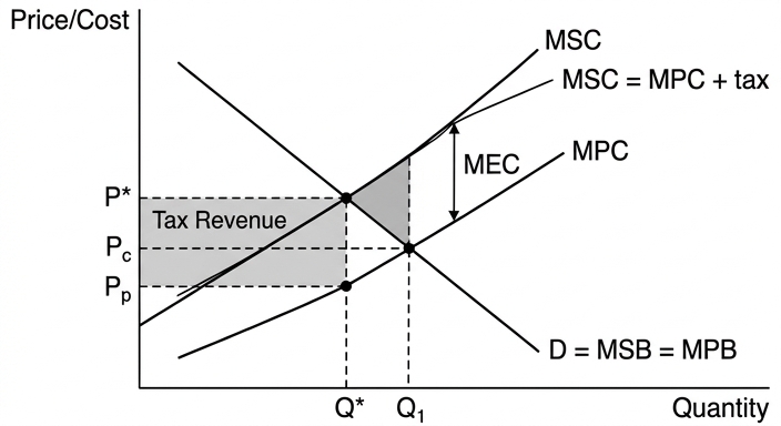
The diagram illustrates the market for a good with negative externalities. The free-market equilibrium at Q1, where MPC = MSB, results in overproduction relative to the social optimum Q*. The tax shifts the supply curve to MPC+tax, aligning with MSC, and the new equilibrium at Q* achieves allocative efficiency.
However, the effectiveness of this policy depends on accurate measurement of the external cost. If the tax is too low, under-correction occurs; if too high, it leads to underproduction and a different deadweight loss. Additionally, indirect taxes can be regressive, disproportionately affecting lower-income consumers. They may also reduce international competitiveness if not coordinated across countries, and they can be evaded through illegal activity.
Pollution Permits (Cap-and-Trade)
A pollution permit system sets a cap on total emissions equal to the socially optimal level of pollution. Permits are allocated (by auction or grandfathering) and can be traded among firms. This creates a market price for pollution, internalising the externality. Firms with low abatement costs will sell permits, while those with high abatement costs will buy them, ensuring that the pollution reduction is achieved at the lowest possible cost. The total quantity of pollution is limited to the cap, so the marginal social cost of pollution is equalised across firms, and the outcome is allocatively efficient.
The success of this policy hinges on setting the cap correctly. If the cap is too high, no improvement in allocative efficiency occurs; if too low, excessive costs are imposed. Effective monitoring and enforcement are required to prevent cheating. The initial allocation of permits raises equity concerns: grandfathering may reward past polluters, while auctioning generates revenue that can be used to offset regressive effects. Moreover, the permit market may be subject to market power or price volatility, reducing efficiency.
Evaluation
Both policies can, in principle, improve allocative efficiency by aligning private costs with social costs. However, their real-world effectiveness is limited by several factors. First, accurate information about the marginal external cost is difficult to obtain, making it hard to set the optimal tax or cap. Second, government failure—such as regulatory capture, political interference, or administrative inefficiency—can lead to suboptimal policy design. Third, distributional effects may create political opposition, undermining implementation. Fourth, both policies may have unintended consequences, such as tax evasion or permit hoarding.
Comparing the two, indirect taxation is simpler to administer but less flexible: it does not guarantee a specific quantity of pollution reduction. Pollution permits provide certainty about the total pollution level but require a well-functioning market and robust enforcement. The choice between them depends on the specific context, including the nature of the externality, the administrative capacity of the government, and the degree of certainty required.
Conclusion
To a significant extent, both indirect taxation and pollution permits can improve allocative efficiency by correcting the market failure caused by negative externalities. However, the extent of improvement is constrained by information asymmetries, government failure, and practical implementation challenges. Therefore, while these policies are theoretically effective, their actual impact on allocative efficiency is partial and context-dependent. A combination of policies, along with complementary measures such as improved information and regulation, may be necessary to achieve a substantial improvement in allocative efficiency.
Indirect taxation and pollution permits can significantly improve allocative efficiency by internalising external costs, but their effectiveness is limited by information problems, government failure, and implementation challenges, so the extent of improvement is partial and context-dependent.
Background Concept
Negative externalities occur when the production or consumption of a good imposes costs on third parties that are not reflected in the market price. For example, a factory emitting pollution imposes health and environmental costs on society. In a free market, firms only consider their private costs (MPC), not the external costs (MEC). The marginal social cost (MSC) is the sum of MPC and MEC. Allocative efficiency is achieved when the marginal social benefit (MSB) equals the marginal social cost (MSC). In the presence of a negative externality, the free-market equilibrium occurs where MPC = MSB, which is at a higher quantity than the socially optimal level where MSC = MSB. This overproduction results in a deadweight welfare loss, indicating allocative inefficiency.
Governments can intervene to internalise the externality, i.e., make private decision-makers face the full social costs. Two common policies are:
- Indirect taxation (Pigouvian tax): A tax per unit equal to the MEC, shifting the MPC curve upward to align with MSC.
- Pollution permits (cap-and-trade): A system where the government sets a cap on total pollution equal to the socially optimal level and issues tradable permits, creating a market price for pollution.
Both policies aim to reduce output to the socially optimal level and eliminate the deadweight loss, thereby improving allocative efficiency.
Understanding the Question
The question asks: "Evaluate, using appropriate diagram(s), the extent to which two policies used to reduce negative externalities can also improve allocative efficiency." This is a 20-mark essay requiring a balanced evaluation. The command word "Evaluate" means you must present both the strengths and weaknesses of the policies and reach a justified conclusion. The phrase "the extent to which" indicates that you should judge how much the policies actually improve allocative efficiency, considering practical limitations. The requirement to use diagram(s) means you must include at least one diagram and explain it fully; failure to do so caps the mark at Level 2.
You need to select two specific policies. This answer chooses indirect taxation and pollution permits, as they are distinct and commonly discussed. The essay should define key terms, explain how each policy works, analyse its impact on allocative efficiency, evaluate its limitations, and then compare them to reach a conclusion.
Approach
- Introduction: Define negative externalities and allocative efficiency. State the two policies to be evaluated.
- First policy: Indirect taxation: Explain the mechanism, draw a diagram showing the externality and the effect of the tax. Analyse how it improves allocative efficiency. Then evaluate its limitations (information, regressive effects, evasion, competitiveness).
- Second policy: Pollution permits: Explain the cap-and-trade mechanism, analyse its impact on allocative efficiency. Evaluate its limitations (setting the cap, enforcement, equity, market power).
- Overall evaluation: Compare the two policies, discuss common limitations (information asymmetry, government failure, distributional effects).
- Conclusion: Provide a justified judgement on the extent to which these policies improve allocative efficiency.
Step-by-Step Reasoning
Step 1: Definitions
- Negative externality: cost imposed on a third party not involved in the transaction.
- Allocative efficiency: occurs when MSB = MSC; resources are allocated to maximise social welfare.
- Deadweight loss: the loss of social surplus due to overproduction.
Step 2: Diagram for negative externality
Draw a standard diagram:
- Axes: Price/Cost (vertical), Quantity (horizontal).
- Downward-sloping demand curve = MSB = MPB (assuming no external benefits).
- Upward-sloping MPC curve (private marginal cost).
- Upward-sloping MSC curve above MPC (MSC = MPC + MEC).
- Free-market equilibrium: where MPC = MSB, at quantity Q1, price P1.
- Social optimum: where MSC = MSB, at quantity Q*, price P*.
- Shade the deadweight loss triangle between Q1 and Q*, bounded by MSC and MSB.
Step 3: Indirect taxation
- A specific tax of amount t = MEC at Q* shifts the MPC curve upward by t to MPC+t.
- If t is set correctly, MPC+t coincides with MSC.
- New equilibrium: where MPC+t = MSB, at Q* and price Pc (consumer price). Producers receive Pp = Pc - t.
- The deadweight loss is eliminated, so allocative efficiency is achieved.
- However, the government must know the exact MEC, which is difficult. If the tax is too low, some deadweight loss remains; if too high, underproduction creates a new deadweight loss.
- Other limitations: regressive (poor spend higher proportion of income on taxed goods), may lead to tax evasion, may harm international competitiveness if other countries do not impose similar taxes.
Step 4: Pollution permits
- The government sets a cap on total emissions equal to Q* (the socially optimal quantity of pollution).
- Permits are issued (e.g., one permit per unit of pollution) and can be traded.
- Firms with low abatement costs will reduce pollution and sell permits; firms with high abatement costs will buy permits. The market price of permits reflects the marginal abatement cost.
- The total pollution is capped at Q*, so the marginal social cost of pollution is equalised across firms, achieving allocative efficiency at minimum cost.
- Limitations: The cap must be set correctly; if too high, no improvement; if too low, excessive costs. Monitoring and enforcement are costly. Initial allocation raises equity issues (grandfathering benefits incumbents, auctioning raises revenue but may face opposition). The permit market may be thin or subject to manipulation.
Step 5: Overall evaluation
- Both policies can theoretically achieve allocative efficiency by internalising the externality.
- However, they face common challenges:
- Information problem: The government rarely knows the exact MEC or the optimal quantity. This leads to either under- or over-correction.
- Government failure: Political pressures, regulatory capture, and administrative inefficiency can result in poorly designed policies.
- Distributional effects: Both policies can disproportionately affect low-income households or certain industries, leading to political opposition and possible reversal.
- Behavioural responses: Firms may evade taxes or find loopholes; permit markets may suffer from speculation or hoarding.
- Comparing the two:
- Tax: Provides price certainty (firms know the cost of pollution), but quantity of pollution is uncertain (firms may choose to pay tax and continue polluting).
- Permits: Provides quantity certainty (total pollution is capped), but price of permits is uncertain (fluctuates with demand).
- The choice depends on context: if the marginal damage of pollution is steep (i.e., small increases cause large harm), quantity certainty is more important; if marginal abatement costs are steep, price certainty is more important.
Step 6: Conclusion
- To a significant extent, both policies can improve allocative efficiency by reducing overproduction and eliminating deadweight loss.
- However, the extent is limited by practical difficulties: imperfect information, government failure, and distributional concerns mean that the theoretical optimum is rarely achieved.
- Therefore, while these policies are valuable tools, their actual impact on allocative efficiency is partial and context-dependent. A combination of policies, along with complementary measures (e.g., improved information, regulation, subsidies for clean alternatives), may be necessary to achieve a substantial improvement.
Key Takeaways
- Negative externalities cause allocative inefficiency due to overproduction.
- Pigouvian taxes and pollution permits are two key policy instruments to internalise externalities.
- Both can theoretically restore allocative efficiency by aligning private and social costs.
- Practical limitations (information, government failure, equity) reduce their effectiveness.
- Evaluation requires a balanced consideration of both theoretical benefits and real-world constraints.
- Diagrams are essential to illustrate the analysis and must be fully explained.
Common Mistakes
- No diagram: The mark scheme explicitly states "Maximum L2 if no diagram". Always include at least one diagram and explain it.
- One-sided evaluation: Only discussing the benefits without limitations loses marks for evaluation. The question asks "evaluate the extent", so both sides are required.
- No conclusion or vague conclusion: The top band requires a justified conclusion that addresses the specific question. A summary without judgement is insufficient.
- Confusing allocative efficiency with productive efficiency: Allocative efficiency is about MSB = MSC; productive efficiency is about producing at minimum average cost. The question specifically asks about allocative efficiency.
- Using incorrect terminology: e.g., saying "social cost" when meaning "external cost", or confusing "tax" with "subsidy".
- Not using the extract: This question has no extract, but if data were provided, it must be used.
Things to Be Careful About
- Label axes and curves clearly on the diagram: Price/Cost on vertical axis, Quantity on horizontal. Label MPC, MSC, MSB, equilibrium points, deadweight loss.
- Explain the diagram in the text: Do not just draw it; describe what it shows and how it supports your analysis.
- Use the correct command word: "Evaluate" requires a judgement, not just description.
- Structure the essay logically: Introduction, analysis of each policy, evaluation, conclusion.
- Be specific about the policies: Choose two distinct policies and explain their mechanisms clearly.
- Consider both sides: For each policy, discuss both how it improves allocative efficiency and its limitations.
- Reach a justified conclusion: State the extent to which the policies improve allocative efficiency, and justify why.
- Avoid overgeneralisation: Use examples where appropriate (e.g., carbon tax, EU Emissions Trading System).
Evaluate the consequences for the price and output of a firm if it changes its objective from profit maximisation to sales maximisation as a response to the principal-agent problem.
Introduction
The principal-agent problem arises when the objectives of a firm's owners (shareholders) differ from those of its managers. Shareholders typically aim to maximise profit, while managers may pursue alternative goals such as sales maximisation to enhance their own status, remuneration, or job security. This essay evaluates the consequences for price and output if a firm changes its objective from profit maximisation to sales maximisation in response to this problem.
Profit Maximisation
Under profit maximisation, the firm produces the level of output where marginal revenue equals marginal cost (MR = MC). The price is then determined from the average revenue (demand) curve. At this output, if average revenue exceeds average cost, the firm earns supernormal profit. This objective results in a relatively higher price and lower quantity compared to other objectives.
Sales Maximisation
Sales maximisation, as an alternative objective, seeks to maximise total revenue (sales) subject to the constraint that the firm earns at least normal profit. This is achieved where average revenue equals average cost (AR = AC), i.e., the firm produces the maximum output that allows it to break even. At this output, the price is again read from the AR curve, but it is lower and the quantity higher than under profit maximisation.
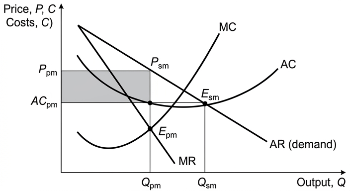
The diagram illustrates a firm with downward-sloping AR and MR curves and U-shaped AC and MC curves. The profit-maximising equilibrium is at output Qpm where MR = MC, with price Ppm on the AR curve. The sales-maximising equilibrium is at output Qsm where AR = AC, with price Psm. Qsm is greater than Qpm, and Psm is lower than Ppm. Under profit maximisation, the firm earns supernormal profit equal to the area between AR and AC at Qpm. Under sales maximisation, the firm earns only normal profit (AR = AC).
Comparison of Price and Output
Changing from profit maximisation to sales maximisation therefore leads to a lower price and a higher output. Consumers benefit from the lower price and greater availability of the good. Producer surplus (supernormal profit) is transferred to consumers as consumer surplus, which may also improve equity if the good is a necessity.
Evaluation
However, the consequences are not unambiguously positive. First, the lower price and higher output may worsen allocative efficiency. Under profit maximisation, price is above marginal cost (P > MC), which is typical of imperfect competition. Under sales maximisation, price is even further from marginal cost (since output is higher and MC may be rising), so the misallocation of resources may increase. Second, the firm forgoes supernormal profit that could have been used for investment in research, development, or expansion, potentially harming long-run dynamic efficiency and growth. Third, the principal-agent problem itself may not be fully resolved: managers may pursue sales maximisation to enhance their own status rather than to benefit shareholders, and the firm may become a target for takeover if its profits are too low. Fourth, the outcome depends on market structure. In a perfectly competitive market, profit maximisation and sales maximisation coincide at the same output (since AR = MR = price, and the firm earns normal profit in the long run), so the change has no effect. The analysis is most relevant to firms with market power, such as monopolies or oligopolies. In such markets, the switch to sales maximisation may also affect the firm's pricing strategies, potentially leading to price wars or collusive behaviour.
Conclusion
In conclusion, changing from profit maximisation to sales maximisation as a response to the principal-agent problem generally results in a lower price and higher output, benefiting consumers in the short run. However, this comes at the cost of reduced allocative efficiency and potentially lower investment, which may harm long-run welfare. The net effect depends on the market structure, the extent of the principal-agent problem, and the time horizon considered. On balance, while sales maximisation may address managerial incentives, it is unlikely to be superior to profit maximisation from a societal perspective unless the firm operates in a highly competitive market where the two objectives converge.
The switch to sales maximisation lowers price and raises output, benefiting consumers but potentially reducing allocative efficiency and long-run investment; the overall welfare effect depends on market structure and the time horizon.
Background Concept
Profit maximisation is the traditional objective of firms, where they choose output such that marginal revenue equals marginal cost (MR = MC). This yields the highest possible profit. In imperfect competition, the firm faces a downward-sloping demand curve, so AR and MR are downward-sloping, and the price is set above marginal cost.
Sales maximisation is an alternative objective where the firm aims to maximise total revenue (sales) subject to earning at least normal profit. This is achieved where average revenue equals average cost (AR = AC). At this output, the firm breaks even, earning only normal profit. The price is lower and output higher than under profit maximisation.
The principal-agent problem arises from the separation of ownership and control in modern corporations. Shareholders (principals) want profit maximisation to maximise their returns, but managers (agents) may have different objectives, such as sales maximisation, to increase their own power, prestige, or remuneration. This conflict can lead managers to pursue sales maximisation even if it reduces profits.
Understanding the Question
The question asks to evaluate the consequences for price and output if a firm changes its objective from profit maximisation to sales maximisation as a response to the principal-agent problem. This means we need to compare the two objectives, explain why the change might occur, and then evaluate the effects on price and output, as well as broader welfare implications. The command word "Evaluate" requires a two-sided analysis: we must consider both the benefits (e.g., lower price, higher output, consumer surplus) and the costs (e.g., allocative inefficiency, reduced investment, potential conflict with shareholders). A justified conclusion is required.
Approach
We will first define the key concepts: profit maximisation, sales maximisation, and the principal-agent problem. Then we will analyse each objective using a cost and revenue diagram, showing the equilibrium price and output under each. We will compare the outcomes and then evaluate the consequences from multiple perspectives: consumers, allocative efficiency, dynamic efficiency, market structure, and the principal-agent problem itself. Finally, we will reach a justified conclusion that addresses the specific question.
Step-by-Step Reasoning
-
Principal-agent problem: In many firms, owners (shareholders) are not involved in day-to-day management. Managers may pursue their own interests, such as higher salaries, job security, or prestige, which may be linked to sales revenue rather than profits. This can lead managers to adopt sales maximisation as an objective.
-
Profit maximisation: The firm produces where MR = MC. In imperfect competition, the demand curve is downward-sloping, so MR lies below AR. The price is set on the AR curve at the profit-maximising output. The firm earns supernormal profit if AR > AC at that output.
-
Sales maximisation: The firm aims to maximise sales revenue subject to a break-even constraint (at least normal profit). This occurs where AR = AC. At this output, the firm earns normal profit. The price is lower and output higher than under profit maximisation.
-
Diagram: Draw a diagram with AR (demand), MR, AC, and MC curves. Mark the profit-maximising output Qpm at MR=MC, with price Ppm on AR. Mark the sales-maximising output Qsm at AR=AC, with price Psm on AR. Qsm > Qpm, Psm < Ppm. Shade the supernormal profit area under profit maximisation (rectangle between AR and AC at Qpm). Under sales maximisation, AR=AC so no supernormal profit.
-
Consequences for price and output: The switch lowers price from Ppm to Psm and raises output from Qpm to Qsm. Consumers benefit from lower price and greater quantity. Consumer surplus increases. If the good is a necessity, this may also improve equity.
-
Evaluation:
- Allocative efficiency: Under profit maximisation, P > MC, indicating underproduction and allocative inefficiency. Under sales maximisation, output is higher, but P is even further from MC (since MC is rising), so the deadweight loss may increase. However, some economists argue that sales maximisation brings output closer to the competitive level, reducing inefficiency. This is debatable.
- Dynamic efficiency: Supernormal profit under profit maximisation can be reinvested in R&D, innovation, and expansion, promoting long-run growth. Sales maximisation sacrifices this profit, potentially reducing dynamic efficiency and the firm's competitiveness over time.
- Principal-agent problem: Sales maximisation may align managers' objectives with their own interests but not necessarily with shareholders'. Shareholders may use performance-related pay or monitoring to align objectives. The change to sales maximisation might be a response to weak corporate governance, but it does not resolve the underlying conflict.
- Market structure: In perfect competition, AR=MR=P, and in long-run equilibrium, firms earn normal profit, so profit maximisation and sales maximisation yield the same output and price. The analysis is most relevant to firms with market power. In oligopoly, sales maximisation might lead to price wars or collusion, affecting industry outcomes.
- Time horizon: In the short run, consumers gain from lower prices. In the long run, reduced investment may harm the firm's survival and the industry's health.
-
Conclusion: The switch to sales maximisation lowers price and raises output, benefiting consumers in the short run. However, it may reduce allocative efficiency and long-run investment. The net welfare effect depends on market structure, the extent of the principal-agent problem, and the time horizon. On balance, sales maximisation is unlikely to be superior to profit maximisation from a societal perspective unless the firm operates in a highly competitive market where the two objectives converge.
Key Takeaways
- Profit maximisation: MR=MC, higher price, lower output, supernormal profit.
- Sales maximisation: AR=AC, lower price, higher output, normal profit.
- Principal-agent problem can lead managers to pursue sales maximisation.
- Consequences: consumer benefit vs allocative inefficiency and reduced investment.
- The effect depends on market structure; in perfect competition, no difference.
- A justified conclusion must weigh both sides.
Common Mistakes
- Confusing sales maximisation with revenue maximisation (MR=0). Sales maximisation is subject to a break-even constraint, so it is AR=AC, not MR=0.
- Forgetting to include the break-even constraint; sales maximisation does not mean producing at any cost; the firm must at least break even.
- Not using a diagram or not explaining it fully. The diagram is crucial for showing the two equilibria.
- One-sided evaluation: only discussing benefits or only costs. The command word "Evaluate" requires both sides.
- No conclusion or a vague conclusion. The top band requires a justified conclusion.
- Ignoring the principal-agent problem context; the question specifically asks for consequences as a response to this problem.
Things to Be Careful About
- Label all axes and curves on the diagram: price/cost on vertical axis, quantity on horizontal axis; AR, MR, AC, MC curves clearly labelled; equilibrium points marked.
- Explain the diagram in the text: what each curve represents, where the equilibria are, and what the shaded area shows.
- Distinguish between short-run and long-run consequences.
- Consider different market structures; the analysis may not apply to perfect competition.
- Ensure the conclusion is justified and directly answers the question: what are the consequences for price and output?
- Use economic terminology accurately: supernormal profit, normal profit, allocative efficiency, dynamic efficiency, consumer surplus, etc.
In periods of rising and persistent inflation, consumers and workers change their expectations of the future rate of inflation.
Evaluate, with the help of a diagram(s), the consequences of these changes of expectations for fiscal policy.
Introduction
Inflation is a sustained increase in the general price level. When inflation becomes persistent, consumers and workers revise their expectations of future inflation, typically based on past experience (adaptive expectations). This fundamentally alters the short-run trade-off between inflation and unemployment and has important consequences for the effectiveness of fiscal policy. The question requires an evaluation of how such changes in expectations affect the ability of fiscal policy to achieve its objectives, particularly reducing unemployment.
Analysis: The expectations-augmented Phillips curve
The traditional Phillips curve suggested a stable inverse relationship between inflation and unemployment. However, the expectations-augmented Phillips curve incorporates the role of expected inflation. In the short run, there is a trade-off: an expansionary fiscal policy (e.g., increased government spending or lower taxes) shifts aggregate demand to the right, raising output and reducing unemployment below the natural rate, but at the cost of higher inflation. This is shown as a movement along the short-run Phillips curve (SRPC).
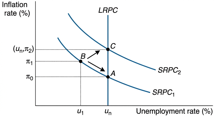
However, as workers and consumers experience higher inflation, they revise their expectations upward. Workers demand higher nominal wages to maintain real wages, and firms pass on the increased costs, shifting the short-run Phillips curve upward (from SRPC1 to SRPC2). The economy returns to the natural rate of unemployment but at a higher rate of inflation. To keep unemployment below the natural rate, inflation must accelerate – the accelerationist hypothesis. Thus, expansionary fiscal policy can only temporarily reduce unemployment; its long-run effect is solely on inflation.
If expectations are rational, agents anticipate the inflationary consequences of fiscal policy and adjust wages and prices immediately. In this case, even the short-run trade-off disappears, and fiscal policy has no real effects from the outset.
Evaluation
The consequences of changing expectations for fiscal policy are significant but contingent on several factors:
- Speed of expectation adjustment: If expectations are sticky (e.g., due to backward-looking behaviour), fiscal policy may have a longer-lasting impact on real output. However, if expectations adjust rapidly, the window for real effects is very short.
- The shape of the aggregate supply curve: In a deep recession with a horizontal SRAS (Keynesian range), expansionary fiscal policy can increase output without much inflation, even if expectations are present. This reduces the cost of using fiscal policy.
- Credibility of policy: If the government and central bank have a credible commitment to low inflation, expectations may not rise as much, preserving some effectiveness of fiscal policy. The opposite holds if credibility is low.
- Supply-side policies: Combining fiscal policy with supply-side reforms can lower the natural rate of unemployment, allowing fiscal expansion to reduce unemployment without generating accelerating inflation. This is a more sustainable approach.
- Historical evidence: The 1970s stagflation demonstrated that expansionary fiscal policy combined with supply shocks led to high inflation and high unemployment, supporting the expectations-augmented Phillips curve. In contrast, the 1990s and 2000s saw low inflation and low unemployment, partly due to credible monetary policy and globalisation, which moderated expectations.
- Other objectives: Fiscal policy may still be used for redistribution, infrastructure, or stabilisation of automatic stabilisers, even if its demand management role is limited.
Conclusion
Changing expectations significantly reduce the ability of fiscal policy to permanently lower unemployment. In the long run, expansionary fiscal policy only results in higher inflation unless the economy is in a recession or accompanied by supply-side improvements. The effectiveness of fiscal policy is therefore highly dependent on the state of expectations, policy credibility, and the economic context. For sustained low unemployment and low inflation, supply-side policies are more appropriate than reliance on demand management.
Changing expectations limit the effectiveness of fiscal policy for demand management; it can only affect inflation in the long run, not real output, unless the economy is in a recession or supply-side reforms are implemented.
Background Concept
This question is about the interaction between inflation expectations and the effectiveness of fiscal policy. The key theoretical framework is the expectations-augmented Phillips curve, which builds on the original Phillips curve (1958) showing an inverse relationship between wage inflation and unemployment. The expectations-augmented version, developed by Friedman and Phelps, incorporates the idea that workers and firms care about real wages, not nominal wages. When inflation rises, workers demand higher nominal wages to maintain their real purchasing power. If they expect inflation to be higher, they will demand even higher wages, shifting the short-run Phillips curve upward. The long-run Phillips curve is vertical at the natural rate of unemployment – there is no trade-off between inflation and unemployment in the long run.
Understanding this helps explain why expansionary fiscal policy (e.g., increased government spending or tax cuts) may only have temporary effects on unemployment and can lead to permanently higher inflation if expectations adapt.
Understanding the Question
The question states: "In periods of rising and persistent inflation, consumers and workers change their expectations of the future rate of inflation." This is a description of adaptive expectations – people extrapolate past inflation into the future. The question asks to evaluate the consequences of these changes of expectations for fiscal policy. The command word is "Evaluate," which requires a two-sided analysis and a justified conclusion. The hint "with the help of a diagram(s)" means a diagram is essential; the mark scheme explicitly caps at Level 2 without one.
The question is a 20-mark undivided essay (modern Paper 4 format). It tests AO1/AO2 (knowledge and analysis – 14 marks) and AO3 (evaluation – 6 marks). The top band for AO3 requires a justified conclusion with developed evaluative comments.
Approach
To answer this question, you should:
- Define key terms – inflation, expectations (adaptive vs rational), natural rate of unemployment, Phillips curve.
- Set up the theoretical framework – explain the expectations-augmented Phillips curve and how expectations change the short-run trade-off.
- Use a diagram – draw the expectations-augmented Phillips curve showing the short-run curves shifting upward as expectations adjust, and the long-run vertical Phillips curve.
- Analyse the consequences for fiscal policy – show that expansionary fiscal policy can only temporarily reduce unemployment; in the long run it leads to higher inflation (the accelerationist hypothesis).
- Evaluate – consider factors that modify this conclusion: the speed of expectation adjustment, the shape of the AS curve (Keynesian vs classical), policy credibility, supply-side policies, historical evidence, and other objectives of fiscal policy.
- Conclusion – state a justified judgement about the overall consequences for fiscal policy, acknowledging conditions under which fiscal policy might still be effective.
Step-by-Step Reasoning
-
Define inflation and expectations: Inflation is a persistent rise in the general price level. Expectations are the beliefs about future inflation. In adaptive expectations, people form expectations based on past inflation: if inflation has been high and rising, they expect it to continue.
-
The expectations-augmented Phillips curve: The short-run Phillips curve (SRPC) shows a negative relationship between inflation and unemployment, given expected inflation. The equation is: π = π^e - β(u - u_n) + supply shocks. The long-run Phillips curve (LRPC) is vertical at the natural rate u_n, where π = π^e.
-
Diagram explanation: Draw a graph with inflation rate on the vertical axis and unemployment rate on the horizontal axis. Draw a vertical LRPC at u_n. Draw a downward-sloping SRPC1 crossing LRPC at point A (low inflation, natural rate). Now suppose the government uses expansionary fiscal policy (e.g., increase spending). This raises aggregate demand, reducing unemployment to u1 < u_n and increasing inflation to π1 (point B on SRPC1). However, because inflation is now higher than expected, workers revise their expectations upward. The SRPC shifts upward to SRPC2, which goes through point C: at the natural rate, inflation is now π2. The economy moves from B to C as nominal wages adjust, returning unemployment to the natural rate but at a higher inflation rate. The path is A → B → C. If the government persists, inflation accelerates.
-
Consequences for fiscal policy: The main consequence is that fiscal policy cannot permanently reduce unemployment below the natural rate. It only creates a temporary boom followed by higher inflation. This is a significant limitation: fiscal policy becomes ineffective as a tool for demand management in the long run. Moreover, if expectations are rational and agents anticipate the policy, even the short-run effect may be negligible.
-
Evaluation:
- Speed of adjustment: If expectations adjust slowly (e.g., because of inertia or backward-looking behaviour), fiscal policy can have a longer-lasting real effect. This is more likely in economies with low financial literacy or rigid labour markets.
- Slack in the economy: If the economy is far below full employment (e.g., in a deep recession with a horizontal AS curve), expansionary fiscal policy can increase output without generating much inflation, because there is spare capacity. Expectations may not rise as strongly because the initial inflation increase is small.
- Policy credibility: If the government is committed to low inflation (e.g., through an independent central bank or a fiscal rule), expectations may not rise as much, preserving the short-run trade-off. Credibility reduces the shift in SRPC.
- Supply-side policies: If fiscal expansion is combined with supply-side reforms that lower the natural rate (e.g., improved education, deregulation), then the LRPC shifts right. This can allow lower unemployment without accelerating inflation, making fiscal policy more effective.
- Historical evidence: The 1970s saw high inflation and high unemployment (stagflation) because expansionary policies combined with oil price shocks and rising expectations led to the upward shift of SRPC. In contrast, the 1990s and 2000s saw low inflation and low unemployment due to credible monetary policy and globalisation, which kept expectations anchored despite economic growth.
- Other objectives: Fiscal policy may still be used for redistribution, infrastructure, or automatic stabilisation. Even if its demand management role is limited, it can improve long-run productivity.
-
Conclusion: The overall consequence is that changing expectations undermine the ability of fiscal policy to reduce unemployment in the long run. However, in the short run or during recessions, fiscal policy can still be effective. The most sustainable approach is to use fiscal policy alongside supply-side reforms to lower the natural rate, rather than relying solely on demand expansion.
Key Takeaways
- Inflation expectations are crucial for the effectiveness of demand management policies.
- The expectations-augmented Phillips curve shows that the long-run trade-off between inflation and unemployment disappears.
- Expansionary fiscal policy can only temporarily reduce unemployment; in the long run it leads to higher inflation.
- The speed of adjustment of expectations and the state of the economy (slack) determine the short-run effectiveness.
- Policy credibility and supply-side policies can mitigate the negative consequences.
- A diagram is essential for full marks; it must be fully explained in the text.
Common Mistakes
- Omitting the diagram: The mark scheme explicitly caps at Level 2 without a diagram. Many students lose marks by not including one.
- One-sided evaluation: Failing to discuss factors that could preserve the effectiveness of fiscal policy (e.g., recessions, credibility) leads to a low evaluation score.
- Confusing the short-run and long-run Phillips curve: Not distinguishing between the temporary and permanent effects is a common error.
- Lack of development: Simply stating that fiscal policy causes inflation without explaining the mechanism of expectations adjustment is insufficient.
- Ignoring the question: The question asks specifically about the consequences of changing expectations for fiscal policy, not just a general discussion of inflation.
- No conclusion: A justified conclusion is required for the top evaluation band. A summary of both sides without a judgement is not enough.
Things to Be Careful About
- Label axes and curves clearly on the diagram: inflation rate on vertical axis, unemployment on horizontal axis, LRPC vertical, SRPC downward sloping, and show the shift.
- Explain the diagram in the text: The diagram alone is not enough; the prose must walk through the shift and the movement along the curves.
- Use the correct terminology: adaptive expectations, natural rate, accelerationist hypothesis, cost-push inflation, demand-pull inflation.
- Distinguish between short-run and long-run: The short-run trade-off exists, but the long-run effect is only on inflation.
- Acknowledge the role of supply-side policies: This strengthens the evaluation and shows depth.
- Be explicit about the conclusion: state clearly whether fiscal policy is effective or not, and under what conditions.
In recent years many countries have joined or established a free trade area (FTA).
Evaluate, with the help of a diagram(s), whether membership of an FTA is always beneficial to a country.
Introduction
A free trade area (FTA) is a bloc of countries that agree to eliminate tariffs and quotas on trade among themselves while each member retains its own trade policies towards non-members. Examples include NAFTA (now USMCA) and ASEAN. This essay evaluates whether membership of an FTA is always beneficial, using a diagram to illustrate the welfare effects and considering both microeconomic and macroeconomic arguments.
Benefits of FTA Membership
The primary benefit of joining an FTA is trade creation. When a country removes tariffs on imports from partner countries, domestic consumers can buy imported goods at a lower price. This increases consumer surplus and allocative efficiency, as resources are redirected towards industries where the country has a comparative advantage. The diagram below shows the domestic market for a good.
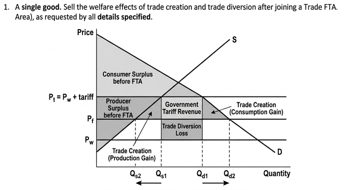
Initially, the country imposes a tariff on all imports, raising the domestic price to Pt (world price Pw plus tariff). Domestic output is Qs1 and consumption is Qd1; the government collects tariff revenue equal to area c. After joining the FTA, tariffs are removed on imports from partner countries, so the domestic price falls to Pf (the partner's price, assumed lower than Pt). Consumption rises to Qd2, domestic output falls to Qs2, and imports increase. Consumer surplus expands by areas a + b + c + d. Producer surplus falls by area a, and government loses tariff revenue c. The net welfare gain is b + d, representing the gains from trade creation (b is the production gain from shifting resources away from inefficient domestic production, and d is the consumption gain from increased consumer surplus).
Additionally, access to a larger market allows firms to exploit economies of scale, lowering average costs and improving productive efficiency. This can lead to lower prices and greater variety for consumers. The removal of barriers also encourages foreign direct investment and technology transfer, boosting long-run growth.
Drawbacks and Limitations
However, membership of an FTA is not always beneficial. A key risk is trade diversion. If the partner country is not the lowest-cost producer, the country may switch from importing from a more efficient non-member (at world price Pw) to a less efficient partner (at Pf > Pw). In the diagram, if Pf is above Pw, the net welfare effect could be negative: the gain from trade creation (b + d) may be outweighed by the loss from trade diversion (the difference between Pf and Pw multiplied by the volume of diverted trade). This is more likely when the FTA's rules of origin are complex or when external tariffs are high.
Other drawbacks include structural unemployment, as domestic industries that cannot compete with partner imports may contract, leading to job losses and adjustment costs. The removal of barriers may also enable countries to 'export' pollution by relocating dirty industries to members with lax environmental standards. Macroeconomic effects depend on the marginal propensity to import; if imports rise faster than exports, the trade balance may worsen, reducing aggregate demand. Furthermore, FTAs can create complex rules of origin that increase administrative costs and may be used as protectionist tools.
Evaluation
Whether an FTA is beneficial depends on several factors. The net welfare effect hinges on the balance between trade creation and trade diversion. An FTA is more likely to be beneficial when member countries are geographically close, have similar levels of development, and when external tariffs are low (reducing the incentive for trade diversion). The price elasticity of demand and supply also matters: the more elastic the curves, the larger the welfare gains from tariff removal. Adjustment costs can be mitigated by complementary policies such as retraining programmes and social safety nets. In the long run, dynamic gains from competition and innovation may outweigh short-run losses. However, for a country with a high-cost manufacturing sector and a comparative advantage in agriculture, joining an FTA with a low-cost manufacturing partner could lead to deindustrialisation and persistent trade deficits.
Conclusion
Membership of an FTA is not always beneficial. It yields net gains when trade creation dominates trade diversion and when the economy can adjust flexibly. However, if trade diversion is significant or if adjustment costs are high, the net effect may be negative. Therefore, the outcome depends on the specific characteristics of the country and its trading partners, and a blanket assertion that FTAs are always beneficial is incorrect.
Membership of an FTA is not always beneficial; it yields net gains when trade creation outweighs trade diversion and when adjustment costs are manageable, but can be harmful if trade diversion dominates or if structural unemployment and environmental dumping are severe.
Background Concept
A free trade area (FTA) is a form of economic integration where member countries eliminate tariffs and quotas on trade among themselves, but each member maintains its own trade policies (tariffs) towards non-members. This is distinct from a customs union, which also has a common external tariff. The key economic concepts are trade creation and trade diversion. Trade creation occurs when a country shifts from high-cost domestic production to lower-cost imports from a partner, increasing allocative efficiency and consumer surplus. Trade diversion occurs when a country shifts from low-cost imports from a non-member to higher-cost imports from a partner, reducing efficiency. The net welfare effect of joining an FTA depends on which effect dominates. Other benefits include economies of scale, increased competition, and technology transfer. Drawbacks include structural unemployment, environmental dumping, and loss of policy autonomy.
Understanding the Question
The question asks to evaluate whether membership of an FTA is always beneficial to a country. The word "always" signals an absolute claim that must be challenged. The command word "Evaluate" requires a two-sided analysis and a justified conclusion. The question also specifies "with the help of a diagram(s)", so a diagram is mandatory and must be fully explained. The essay is worth 20 marks, with AO1+AO2 out of 14 and AO3 out of 6. The top band requires detailed knowledge, developed analysis, accurate use of diagrams, and a justified conclusion. The answer must address both microeconomic and macroeconomic effects, and consider conditions under which the net benefit may be positive or negative.
Approach
The essay will first define an FTA and outline the theoretical benefits using a diagram to illustrate trade creation and consumer surplus gains. It will then present the counter-arguments: trade diversion, structural unemployment, environmental concerns, and macroeconomic risks. The evaluation will weigh these factors, discussing the role of elasticities, the balance between trade creation and diversion, adjustment policies, and dynamic effects. The conclusion will state that membership is not always beneficial; it depends on specific circumstances.
Step-by-Step Reasoning
- Definition and context: Start by defining an FTA and giving examples. This establishes knowledge.
- Diagram and trade creation: Draw the diagram. Explain the initial situation with a tariff: domestic price Pt, output Qs1, consumption Qd1, imports, government revenue. Then show the effect of joining the FTA: tariff removed on partner imports, price falls to Pf (lower than Pt). New output Qs2, consumption Qd2, imports increase. Identify the changes in consumer surplus (increase), producer surplus (decrease), government revenue (loss). The net gain is the sum of the production and consumption triangles (b+d). This is trade creation.
- Other benefits: Discuss economies of scale: access to a larger market reduces average costs. Increased competition leads to lower prices and innovation. Foreign direct investment may increase. These are dynamic gains.
- Trade diversion: Explain that if the partner is not the lowest-cost producer, the country may switch from importing from the world at Pw to importing from the partner at Pf > Pw. This creates a welfare loss (the rectangle of diverted trade). The net effect could be negative if trade diversion outweighs trade creation.
- Structural unemployment: Import-competing industries contract, causing job losses. Labour may not be mobile, leading to hysteresis and long-term unemployment. Adjustment costs can be significant.
- Environmental dumping: Countries with lax environmental standards may attract polluting industries, worsening global pollution. This is a negative externality.
- Macroeconomic effects: If imports rise faster than exports, the trade balance deteriorates, reducing aggregate demand. However, if the FTA boosts export competitiveness, net exports may rise. The multiplier effect can amplify positive or negative changes.
- Evaluation: The net benefit depends on the balance of trade creation vs diversion. Factors: geographic proximity, similarity of economies, level of external tariffs, elasticities of demand and supply. Adjustment policies (retraining, safety nets) can mitigate costs. Dynamic gains may outweigh short-run losses. For a developing country, joining an FTA with a more advanced partner could lead to deindustrialisation if it lacks comparative advantage in manufacturing.
- Conclusion: Membership is not always beneficial. It is beneficial when trade creation dominates and adjustment is smooth; harmful when trade diversion dominates or adjustment costs are high. Therefore, the statement is false; the outcome is conditional.
Key Takeaways
- FTAs eliminate internal tariffs but allow independent external tariffs.
- Trade creation improves welfare; trade diversion reduces it.
- The net welfare effect depends on the balance between these two.
- Other factors: economies of scale, competition, FDI, structural unemployment, environmental effects.
- A diagram is essential to illustrate the welfare changes.
- Evaluation must consider both micro and macro effects and reach a justified conclusion.
Common Mistakes
- One-sided answer: only discussing benefits or only drawbacks, which loses all evaluation marks.
- No diagram or diagram not explained: capped at Level 2.
- Confusing FTA with customs union or common market.
- Ignoring trade diversion: a key counter-argument.
- Vague conclusion: "it depends" without specifying on what.
- Not addressing the "always" in the question: failing to challenge the absolute.
- Using irrelevant diagrams (e.g., PPF, AD/AS) without linking to FTA.
Things to Be Careful About
- Label all axes, curves, and prices on the diagram.
- Explain the diagram fully in prose; do not just draw it.
- Use correct terminology: trade creation, trade diversion, consumer surplus, producer surplus, allocative efficiency.
- Distinguish between short-run adjustment costs and long-run dynamic gains.
- Consider both micro (welfare) and macro (AD, employment) effects.
- Ensure the conclusion directly answers the question: is it always beneficial? No.
- Support evaluation with economic reasoning, not just opinion.