Economics 9708/33 — October/November 2024
Cambridge A-Level · A Level Multiple Choice · answer key with instant marking and worked solutions
Topics Market Structures · Effectiveness of Macroeconomic Policies · Characteristics of Countries at Different Levels of Development · Efficiency and Market Failure · Wage Determination and Labour Market Intervention · Employment and Unemployment · +17 more
Tap an option under each question to check it — your score builds as you go.
A rational consumer chooses what quantities of two products Y and Z to purchase with a given income.
MUY and MUZ are the additions to total utility that would result if the consumer were to purchase an additional unit of each product.
PY and PZ are the current prices of the two products.
Which outcome would represent consumer equilibrium?
Options
A when MUY = MUZ
B when MUY × PY = MUZ × PZ
C when MUY × PZ = MUZ × PY
D it is not possible to tell from the information available
Reasoning
Consumer equilibrium occurs when the marginal utility per unit of money spent is equal across all goods. For goods Y and Z, this condition is:
MUY / PY = MUZ / PZ
Cross-multiplying gives:
MUY × PZ = MUZ × PY
This is option C.
Answer
C
C
Background Concept
The equi-marginal principle states that a rational consumer maximises total utility from a given income by allocating spending so that the marginal utility per unit of currency (the 'marginal utility per dollar') is equal across all goods. If MUY / PY > MUZ / PZ, the consumer gains more utility per dollar from Y than from Z, so they should buy more Y and less Z until equality is restored. The reverse holds if MUY / PY < MUZ / PZ.
Understanding the Question
The question asks which algebraic expression represents consumer equilibrium for a rational consumer choosing between two goods Y and Z, given their marginal utilities (MUY, MUZ) and prices (PY, PZ). The correct condition is the equi-marginal principle: the marginal utility per unit of money spent is equal across goods.
Approach
Start from the standard equilibrium condition: MUY / PY = MUZ / PZ. Rearrange algebraically to match one of the given options. Cross-multiply to eliminate the denominators, then compare with A, B, C, and D.
Step-by-Step Reasoning
-
The equi-marginal condition for two goods Y and Z is:
MUY / PY = MUZ / PZ -
Multiply both sides by PY × PZ:
MUY × PZ = MUZ × PY -
This matches option C exactly.
-
Option A (MUY = MUZ) is incorrect because it ignores prices — equal marginal utilities do not guarantee equal utility per dollar unless prices are equal.
-
Option B (MUY × PY = MUZ × PZ) is incorrect — it would imply MUY / PZ = MUZ / PY, which is not the equilibrium condition.
-
Option D is incorrect because the information is sufficient to determine the condition.
Key Takeaways
- Consumer equilibrium for a rational consumer requires equal marginal utility per unit of money spent across all goods.
- The algebraic form is MUY / PY = MUZ / PZ, which can be rearranged to MUY × PZ = MUZ × PY.
- Always check the units: the condition equates 'utils per dollar', not 'utils' alone.
Common Mistakes
- Choosing A (MUY = MUZ) — this ignores the role of prices and is only correct if PY = PZ.
- Choosing B (MUY × PY = MUZ × PZ) — this is a common algebraic error from misapplying cross-multiplication.
- Thinking the information is insufficient (D) — the equi-marginal principle is a standard result, so the condition is fully determined.
Things to Be Careful About
- Remember that the equilibrium condition is about marginal utility per unit of money, not total utility or marginal utility alone.
- When rearranging, ensure you multiply both sides by the product of the prices correctly: MUY / PY = MUZ / PZ → MUY × PZ = MUZ × PY.
Which statement about indifference curves is not correct?
Options
A Indifference curves are usually convex to the origin of the diagram.
B Indifference curves can intersect each other.
C The consumer always prefers a higher indifference curve to a lower one.
D The slope of the indifference curve represents the marginal rate of substitution.
Reasoning
Indifference curves are convex to the origin (A), cannot intersect (B is false), higher curves are preferred (C), and the slope is the marginal rate of substitution (D). Therefore, the incorrect statement is B.
Answer
B
B
Background Concept
Indifference curves represent combinations of two goods that give the consumer the same level of utility. They are a key tool in microeconomics to analyse consumer preferences. The properties include: downward sloping (if both goods are desirable), convex to the origin (diminishing marginal rate of substitution), cannot intersect (transitivity), higher curves represent higher utility, and the slope is the marginal rate of substitution (MRS).
Understanding the Question
The question asks which statement is NOT correct. We need to evaluate each option against the standard properties of indifference curves.
Approach
Recall the four properties and test each option. Option B claims indifference curves can intersect, which violates the transitivity assumption of consumer preferences.
Step-by-Step Reasoning
- Option A: Indifference curves are usually convex to the origin because of the diminishing marginal rate of substitution. This is correct.
- Option B: If two indifference curves intersect, at the intersection point the consumer would have the same utility from both curves, implying they are the same indifference curve. This violates transitivity and the definition of indifference curves. Therefore, this statement is incorrect.
- Option C: A higher indifference curve represents a combination with more of at least one good, so it yields higher utility. This is correct.
- Option D: The slope of the indifference curve is the marginal rate of substitution (MRS), which shows the rate at which the consumer is willing to trade one good for another. This is correct.
Key Takeaways
Indifference curves are a fundamental tool in consumer theory. Their properties—downward slope, convexity, non-intersection, and higher curves representing higher utility—are essential for understanding consumer choice and deriving demand curves.
Common Mistakes
A common mistake is thinking that indifference curves can intersect. They cannot, because that would imply inconsistent preferences. Another mistake is confusing convexity with concavity; indifference curves are convex to the origin due to diminishing MRS.
Things to Be Careful About
Remember that indifference curves are typically convex, but there are exceptions (e.g., perfect substitutes are straight lines, perfect complements are L-shaped). However, the question says "usually convex", which is correct. Also, ensure you understand that the slope is the MRS, not the ratio of prices (that is the slope of the budget line).
A firm increases its production.
When will this result in allocative efficiency?
Options
A when the cost of producing the last extra unit equals the value the consumers place on it
B when the cost of producing the last extra unit is at a minimum
C when the total cost of production equals the value that consumers place on the total product
D when the total revenue reaches a maximum
Answer
Allocative efficiency occurs when the price consumers are willing to pay for the last unit (marginal benefit) equals the marginal cost of producing it. This is option A: when the cost of producing the last extra unit equals the value the consumers place on it.
A
Background Concept
Allocative efficiency is a key concept in microeconomics. It describes a situation where resources are distributed in a way that maximises the total welfare (consumer surplus plus producer surplus) in a market. The condition for allocative efficiency is that the price consumers are willing to pay for the last unit produced (which reflects the marginal benefit they receive) is exactly equal to the marginal cost of producing that unit. In a perfectly competitive market, this condition is automatically met at the equilibrium price and quantity because the market price equals both marginal cost and marginal benefit.
Understanding the Question
The question asks: when will an increase in production by a firm result in allocative efficiency? The key is to identify the correct condition among the four options. The question tests the precise definition of allocative efficiency, distinguishing it from other concepts like productive efficiency (minimum average cost) or revenue maximisation.
Approach
Recall the definition of allocative efficiency: it is achieved when the marginal cost (MC) of producing the last unit equals the marginal benefit (MB) that consumers derive from it. In a market, the price consumers pay is a measure of their marginal benefit. Therefore, the condition is P = MC. Now evaluate each option against this definition.
Step-by-Step Reasoning
-
Option A: "when the cost of producing the last extra unit equals the value the consumers place on it". This is exactly the definition of allocative efficiency. The "cost of the last extra unit" is marginal cost (MC). The "value consumers place on it" is the marginal benefit (MB), which is reflected in the price they are willing to pay. So this is correct.
-
Option B: "when the cost of producing the last extra unit is at a minimum". This describes productive efficiency, not allocative efficiency. Productive efficiency occurs when a firm produces at the lowest point on its average cost curve (minimum AC). It is a different concept.
-
Option C: "when the total cost of production equals the value that consumers place on the total product". This compares total cost with total benefit. Allocative efficiency is about the marginal unit, not the total. Even if total cost equals total benefit, the marginal condition might not hold, so this is not the correct definition.
-
Option D: "when the total revenue reaches a maximum". Total revenue is maximised where marginal revenue is zero. This is a firm's revenue objective, not a condition for allocative efficiency. Allocative efficiency is about social welfare, not a firm's revenue.
Key Takeaways
- Allocative efficiency is defined by the equality of marginal cost and marginal benefit (P = MC in a competitive market).
- It is distinct from productive efficiency (minimum AC) and from revenue or profit maximisation.
- The question tests the ability to recall the precise definition and to distinguish it from related but different concepts.
Common Mistakes
- Confusing allocative efficiency with productive efficiency (option B). Productive efficiency is about producing at minimum average cost, not about matching marginal cost to consumer value.
- Thinking in terms of totals (option C) rather than margins. Allocative efficiency is a marginal condition.
- Associating efficiency with revenue maximisation (option D). Revenue maximisation is a firm objective, not a welfare criterion.
Things to Be Careful About
- Always focus on the word "marginal" or "last extra unit" when thinking about allocative efficiency.
- Remember that in a perfectly competitive market, the equilibrium automatically satisfies allocative efficiency because P = MC. In other market structures, firms may produce where P > MC, indicating underallocation of resources to that good.
The table shows a firm’s revenue and costs at different levels of output.
| output | marginal revenue | average revenue | marginal cost | average total cost |
|---|---|---|---|---|
| 1 | 125 | 125 | 90 | 140 |
| 2 | 85 | 105 | 40 | 90 |
| 3 | 45 | 85 | 45 | 75 |
| 4 | 25 | 70 | 95 | 80 |
| 5 | 20 | 60 | 130 | 90 |
What is the firm’s total supernormal profit at the profit-maximising level of output?
Options
A -15
B 10
C 30
D 120
Working
Profit is maximised where MR = MC. From the table, MR = MC = 45 at output = 3.
At output = 3:
- AR = 85, so TR = AR × Q = 85 × 3 = 255
- ATC = 75, so TC = ATC × Q = 75 × 3 = 225
Supernormal profit = TR – TC = 255 – 225 = 30
Answer
C
C
Background Concept
Supernormal profit (also called economic profit or abnormal profit) is the profit earned above the minimum required to keep a firm in business (normal profit). It is calculated as total revenue (TR) minus total cost (TC), where total cost includes both explicit costs and the opportunity cost of the owner's resources (normal profit). A firm maximises profit by producing the output level at which marginal revenue (MR) equals marginal cost (MC). This rule applies to all firms, regardless of market structure.
Understanding the Question
The question provides a table of a firm's revenue and cost data at five output levels. The columns are: output (Q), marginal revenue (MR), average revenue (AR), marginal cost (MC), and average total cost (ATC). The task is to find the firm's total supernormal profit at the profit-maximising level of output. The answer is one of four multiple-choice options.
Approach
- Identify the profit-maximising output by finding where MR = MC.
- At that output, calculate total revenue (TR = AR × Q).
- Calculate total cost (TC = ATC × Q).
- Subtract TC from TR to get supernormal profit.
- Match the result to the correct option.
Step-by-Step Reasoning
Step 1: Find the profit-maximising output.
The profit-maximising condition is MR = MC. Scan the MR and MC columns:
- Q=1: MR=125, MC=90 (MR > MC, increase output)
- Q=2: MR=85, MC=40 (MR > MC, increase output)
- Q=3: MR=45, MC=45 (MR = MC, profit-maximising)
- Q=4: MR=25, MC=95 (MR < MC, profit falls if output increases)
- Q=5: MR=20, MC=130 (MR < MC, profit falls further)
Thus, the profit-maximising output is Q = 3.
Step 2: Calculate total revenue at Q = 3.
AR at Q=3 is 85. TR = AR × Q = 85 × 3 = 255.
Step 3: Calculate total cost at Q = 3.
ATC at Q=3 is 75. TC = ATC × Q = 75 × 3 = 225.
Step 4: Calculate supernormal profit.
Supernormal profit = TR – TC = 255 – 225 = 30.
Step 5: Select the correct option.
Option C is 30.
Key Takeaways
- The profit-maximising rule MR = MC applies universally.
- Supernormal profit is TR – TC, where TC includes normal profit.
- When given average values (AR, ATC), multiply by quantity to get totals.
- Always check that the MR = MC point is indeed the highest profit (not a loss-minimising point).
Common Mistakes
- Using the wrong output: Some students might mistakenly use the output where TR is highest or where AR is highest, rather than where MR = MC.
- Confusing average and total: Forgetting to multiply AR or ATC by Q to get TR or TC.
- Misreading the table: The table uses 'marginal revenue' and 'average revenue' – ensure you use the correct column for each calculation.
- Incorrect profit calculation: Subtracting MC from MR at the chosen output gives marginal profit, not total profit.
Things to Be Careful About
- The MR = MC condition identifies the profit-maximising output, but you must verify that profit is positive (or at least not lower at adjacent outputs). Here, at Q=3, TR > TC, so supernormal profit is positive.
- The table provides ATC, not just TC. Always multiply ATC by Q to get TC.
- The answer is a number, not a letter – match it to the options carefully.
- Units: all figures are in the same currency unit (presumably dollars or pounds), so the profit is 30 of that unit.
Which diagram shows a monopolistically competitive firm in long-run equilibrium?
Options
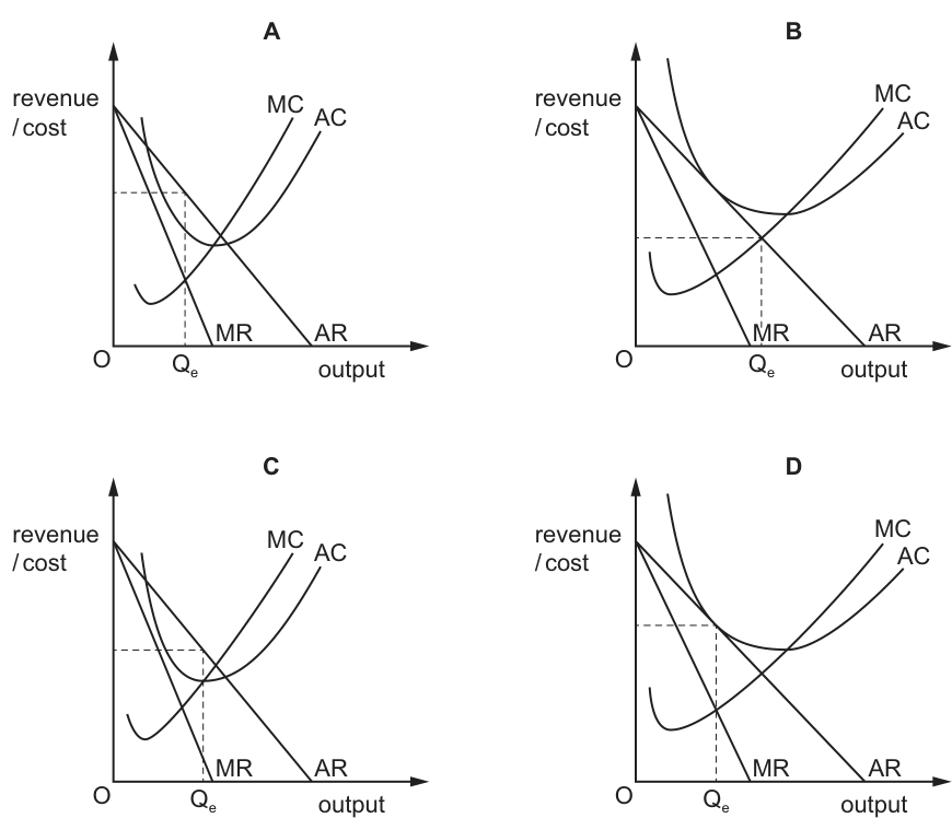
Reasoning
In monopolistic competition, long-run equilibrium is reached when firms make only normal profit (zero economic profit). This occurs where average revenue (AR) equals average cost (AC), meaning the AC curve is tangent to the AR curve. Unlike perfect competition, this tangency does not occur at the minimum point of the AC curve, reflecting excess capacity. The profit-maximising output is determined where marginal revenue equals marginal cost (MR = MC). Diagram D shows the AC curve tangent to the downward-sloping AR curve, indicating normal profit, while output is set where MR = MC. The other diagrams are incorrect: Diagram A shows a loss (AC above AR), Diagram B shows the tangency at the minimum of AC (characteristic of perfect competition, not monopolistic competition), and Diagram C shows supernormal profit (AC below AR).
Answer
D
D
Background Concept
Monopolistic competition is a market structure characterised by many firms selling differentiated products, with free entry and exit in the long run. Key features include downward-sloping demand (AR) and marginal revenue (MR) curves because each firm has some price-setting power due to product differentiation, yet faces competition from close substitutes.
In the short run, a firm can make supernormal profit, normal profit, or a loss depending on the relationship between AR and AC at the profit-maximising output (where MR = MC). However, the defining feature of the long-run equilibrium is the elimination of supernormal profit through free entry and exit. When existing firms make supernormal profit, new firms enter the market, capturing some demand and shifting individual firms' demand curves leftward until AR is just tangent to AC. At this point, firms make only normal profit (zero economic profit), and there is no incentive for further entry or exit.
A crucial distinction from perfect competition is that in monopolistic competition, the tangency between AR and AC occurs not at the minimum point of the AC curve, but to the left of it. This means the firm operates with excess capacity—it could produce more at a lower average cost, but chooses not to because the MR from additional output would be less than the MC.
Understanding the Question
The question asks you to identify which of four diagrams represents a monopolistically competitive firm in long-run equilibrium. This requires you to recognise two simultaneous conditions: (1) the firm is making normal profit (AR = AC), and (2) output is determined by the profit-maximising rule MR = MC. The diagram must also reflect the monopolistically competitive market structure, meaning the AR curve is downward sloping and the AC curve is U-shaped, with the tangency between AR and AC occurring at a point where AC is still falling (or at least not at its minimum).
Approach
To solve this, evaluate each diagram against the long-run equilibrium conditions:
- Check whether the firm makes normal profit (AR = AC), supernormal profit (AR > AC), or a loss (AR < AC) at the output Qe where MR = MC.
- Check whether the AC curve is tangent to AR at Qe.
- Check whether the tangency occurs at the minimum of AC (which would indicate perfect competition, not monopolistic competition).
Diagram A shows AC above AR at Qe, indicating a loss. Diagram C shows AC below AR at Qe, indicating supernormal profit. Both are short-run positions, not long-run equilibrium. Diagram B shows AC tangent to AR at Qe, but if this tangency occurs at the minimum of the AC curve, it represents perfect competition long-run equilibrium. Diagram D shows AC tangent to AR (normal profit) with the tangency occurring at a point indicating excess capacity, consistent with monopolistic competition.
Step-by-Step Reasoning
-
Profit-maximising output: In all market structures, a firm maximises profit (or minimises loss) where MR = MC. In the diagrams, this determines the output level Qe.
-
Normal profit condition: In the long run, monopolistic competition drives economic profit to zero. This means total revenue equals total cost, or equivalently, average revenue equals average cost (AR = AC) at the profit-maximising output. Graphically, the AC curve must be tangent to the AR curve at Qe.
-
Excess capacity: Unlike perfect competition, where long-run equilibrium occurs at the minimum of the AC curve (productive efficiency), monopolistic competition results in the firm producing on the downward-sloping portion of the AC curve. The AC curve is tangent to the AR curve to the left of the minimum AC, indicating the firm could lower its average cost by increasing output, but it does not do so because the MR from extra output would be below MC.
-
Evaluating the options:
- Diagram A: At Qe, the AC curve lies above the AR curve. The firm is making an economic loss. This is not long-run equilibrium.
- Diagram B: The AC curve is tangent to the AR curve at Qe, but this appears to occur at the minimum point of the AC curve. This is the long-run equilibrium condition for perfect competition, not monopolistic competition.
- Diagram C: At Qe, the AC curve lies below the AR curve. The firm is making supernormal profit. This is a short-run equilibrium position.
- Diagram D: The AC curve is tangent to the AR curve, indicating normal profit. The tangency occurs at a point where AC is still falling (or not at its minimum), reflecting the excess capacity characteristic of monopolistic competition. This represents the correct long-run equilibrium.
Key Takeaways
- In monopolistic competition long-run equilibrium, firms make normal profit (AR = AC) and produce where MR = MC.
- The AC curve is tangent to the AR curve, but not at the minimum of AC (excess capacity).
- This contrasts with perfect competition, where long-run equilibrium occurs at the minimum of the AC curve.
- Short-run equilibria can involve supernormal profit (C) or losses (A), but these are eliminated by entry or exit.
Common Mistakes
- Confusing monopolistic competition with perfect competition: Students often select the diagram where AC is tangent to AR at the minimum of AC (Diagram B). This is perfect competition, not monopolistic competition.
- Ignoring the tangency condition: Selecting a diagram where AR = AC but they intersect rather than are tangent (not applicable here, but a common error in other questions).
- Selecting short-run positions: Choosing diagrams showing supernormal profit (C) or losses (A), which are short-run outcomes, not long-run equilibrium.
- Misidentifying the profit-maximising output: Forgetting that Qe is always determined by MR = MC, not by the AR = AC condition.
Things to Be Careful About
- Ensure you identify the tangency between AR and AC, not just intersection. Tangency is required for normal profit in long-run equilibrium because any intersection would imply that at nearby outputs, profit could be higher or lower, contradicting equilibrium.
- Check the position of the tangency relative to the minimum of the AC curve. If the tangency is at the minimum of AC, the diagram shows perfect competition, not monopolistic competition.
- Remember that in monopolistic competition, the AR curve is downward sloping, so the firm has some price-setting power, but free entry ensures only normal profit in the long run.
In a perfectly contestable market, entries and exits are cost-free.
In reality, why is this not the case with some firms in contestable markets?
Options
A Firms cannot recover all fixed costs if they cease operations.
B Firms in the industry all operate at the equilibrium level of output.
C Large firms do not have to increase capital to grow.
D Multinational companies always benefit from economies of scale.
Reasoning
A perfectly contestable market requires that there are no barriers to entry or exit, meaning all costs are recoverable upon exit (no sunk costs). In reality, many firms incur fixed costs that are sunk—they cannot be recovered if the firm ceases operations. Therefore, entries and exits are not cost-free, making the market not perfectly contestable.
Answer
A
A
Background Concept
Contestable markets are markets where entry and exit are completely free, with no sunk costs. Firms can enter when supernormal profits exist and exit without loss if profits fall. Potential competition forces existing firms to behave efficiently, producing at minimum average cost and earning only normal profit. The key condition is cost-free exit, which requires that all fixed costs are recoverable. In reality, many fixed costs are sunk—they cannot be recovered upon exit (e.g., advertising, specialised machinery, training costs). These sunk costs act as a barrier to exit, reducing contestability and allowing incumbent firms to earn supernormal profits in the short run.
Understanding the Question
The question asks: why, in reality, is it not the case that entries and exits are cost-free even in contestable markets? It tests your understanding that the concept of perfect contestability is an ideal, not a description of real markets. The correct answer is A: "Firms cannot recover all fixed costs if they cease operations." This directly identifies sunk costs as the obstacle. Option B refers to equilibrium output, which is irrelevant to entry and exit costs. Option C is false because large firms often do need to increase capital to grow, but this does not relate to exit costs. Option D is a statement about economies of scale that is not universally true and is unrelated to entry/exit costs.
Approach
First, recall the definition of a perfectly contestable market: no barriers to entry or exit, and no sunk costs. This implies that all costs are recoverable upon exit. Then examine each option: A correctly matches the idea that some fixed costs are not recoverable (sunk costs). B is about output, not costs. C is about growth, not exit. D is about economies of scale, not entry/exit costs. Therefore, A is the only option that explains why entries and exits are not cost-free.
Step-by-Step Reasoning
-
A perfectly contestable market requires cost-free entry and exit. This means that if a firm leaves the market, it must be able to recover all its costs. If there are sunk costs, then exit is not cost-free because the firm cannot recover those costs.
-
In practice, many fixed costs are sunk: advertising expenditure, research and development, firm-specific training, and machinery that cannot be resold. These costs are incurred and cannot be recouped if the firm exits.
-
Option A states: "Firms cannot recover all fixed costs if they cease operations." This is the definition of sunk costs and directly explains why exit is not cost-free.
-
Option B: "Firms in the industry all operate at the equilibrium level of output." This is a possible outcome of contestability but does not explain why entry/exit is not cost-free. It is not relevant to the question.
-
Option C: "Large firms do not have to increase capital to grow." This is generally false; firms often need to increase capital to expand. Moreover, it does not address exit costs.
-
Option D: "Multinational companies always benefit from economies of scale." This is not always true and is unrelated to entry/exit costs in contestable markets.
Therefore, the correct answer is A.
Key Takeaways
- Perfect contestability requires no sunk costs, meaning all costs must be recoverable upon exit.
- Real-world markets almost always have some sunk costs, making them at best imperfectly contestable.
- Sunk costs act as a barrier to exit, which allows incumbent firms to earn supernormal profits in the short run.
- The concept of contestability is useful for understanding how potential competition can influence firm behaviour even in concentrated markets.
Common Mistakes
- Confusing contestable markets with perfect competition. Contestable markets do not require many firms; potential competition is sufficient.
- Thinking that contestability requires cost-free entry only, ignoring cost-free exit. Both are required, and exit is often the more important condition.
- Failing to distinguish between fixed costs (recoverable) and sunk costs (non-recoverable). All sunk costs are fixed, but not all fixed costs are sunk.
- Selecting option B or D because they sound relevant but do not directly address the cost of exit.
Things to Be Careful About
- Remember that contestable market theory emphasises the importance of potential competition rather than actual market structure.
- Sunk costs are a barrier to exit, which in turn can deter entry because firms know they cannot exit without loss.
- In multiple-choice questions, read each option carefully to see which one directly answers the specific question posed.
- Avoid general statements that are not directly tied to the condition of cost-free entry/exit.
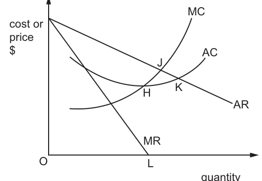
Which points show where each maximisation objective occurs?
Options
| revenue maximisation | sales maximisation | |
|---|---|---|
| A | J | L |
| B | L | K |
| C | J | K |
| D | L | H |
Reasoning
Revenue maximisation occurs where marginal revenue (MR) is equal to zero, as total revenue is maximised when the additional revenue from selling an extra unit of output is zero. On the diagram, MR intersects the horizontal (quantity) axis at point L, so revenue maximisation occurs at quantity L.
Sales maximisation occurs where total revenue equals total cost, which is where average revenue (AR) equals average cost (AC) (the break-even point, the maximum quantity the firm can sell without making a loss). On the diagram, AR and AC intersect at point K, so sales maximisation occurs at point K.
This matches option B.
Answer
B
B
Background Concept
Firms may pursue objectives other than profit maximisation. Two common alternative objectives are revenue maximisation and sales maximisation:
- Revenue maximisation: The firm aims to maximise its total revenue (TR = price × quantity). Total revenue is maximised at the quantity where marginal revenue (MR, the additional revenue from selling one more unit of output) is equal to zero. For quantities below this point, MR is positive, so selling more units increases total revenue; for quantities above this point, MR is negative, so selling more units reduces total revenue.
- Sales maximisation: The firm aims to sell as much output as possible without making a loss. This occurs at the quantity where total revenue equals total cost, which is equivalent to the point where average revenue (AR, the price per unit received by the firm) equals average cost (AC, the cost per unit of producing output). At this point, the firm makes normal profit (zero economic profit), so it is the maximum quantity it can sell while remaining financially viable.
Understanding the Question
The question presents a standard cost and revenue diagram for a firm with market power (evidenced by the downward-sloping AR and MR curves, indicating the firm is not a price-taking perfect competitor). The diagram includes a U-shaped AC curve and an upward-sloping MC curve, with four labelled points: H (minimum AC), J (intersection of MC and AR), K (intersection of AR and AC), and L (the quantity where MR = 0). The question asks you to match the two objectives (revenue maximisation first, then sales maximisation) to the correct points from the options provided.
Approach
To answer this, first recall the exact diagrammatic conditions for each of the two objectives, then locate these conditions on the given diagram:
- For revenue maximisation: The defining condition is MR = 0.
- For sales maximisation: The defining condition is AR = AC (the break-even point).
Once you have identified the correct points for each objective, match them to the option that lists revenue maximisation first, then sales maximisation.
Step-by-Step Reasoning
- First, identify the revenue maximisation point: Revenue is maximised where MR = 0. On the diagram, the MR curve slopes downward and crosses the horizontal (quantity) axis at point L. At this quantity, the additional revenue from selling one more unit is zero, so total revenue is at its maximum. This eliminates options A and C, which incorrectly list J as the revenue maximisation point (J is where MC = AR, the profit-maximising point for a firm seeking to maximise profit, not revenue).
- Next, identify the sales maximisation point: Sales are maximised at the highest quantity the firm can sell without making a loss, which is where AR = AC (total revenue = total cost, so the firm earns normal profit). On the diagram, the AR curve intersects the U-shaped AC curve at point K. This eliminates option D, which incorrectly lists H as the sales maximisation point (H is the minimum point of the AC curve, where MC intersects AC, which is the productively efficient point, not the sales maximisation point).
- The only remaining option is B, which correctly lists L for revenue maximisation and K for sales maximisation.
Key Takeaways
- The key condition for revenue maximisation is MR = 0, which corresponds to the point where the MR curve meets the quantity axis on a cost and revenue diagram.
- The key condition for sales maximisation is AR = AC, the break-even point where the firm makes normal profit, allowing it to sell the maximum possible quantity without loss.
- Always match objectives to their exact defining conditions, rather than confusing them with other points on the diagram (e.g., profit maximisation occurs where MR = MC, which is a different point entirely).
Common Mistakes
- Confusing revenue maximisation with profit maximisation: Profit maximisation occurs where MR = MC (point J on this diagram), not where MR = 0. Selecting J as the revenue maximisation point would lead to the wrong option.
- Confusing sales maximisation with productive efficiency: The minimum point of the AC curve (point H) is the productively efficient output, not the sales maximisation point. Sales maximisation is defined by the break-even condition (AR = AC), not minimum average cost.
- Mismatching the order of objectives: The question asks for revenue maximisation first, then sales maximisation. Even if you identify the correct points, selecting the option that lists them in the wrong order will be incorrect.
Things to Be Careful About
- Verify the labels on the diagram carefully: MR is the steeper downward-sloping curve, AR is the flatter downward-sloping curve, AC is the U-shaped curve, and MC is the upward-sloping curve.
- Remember that revenue maximisation is not the same as profit maximisation: the revenue-maximising quantity is always higher than the profit-maximising quantity, because the firm will keep selling more units even when MR is below MC, as long as MR is positive, to increase total revenue.
- Sales maximisation is always at a quantity higher than the profit-maximising quantity, because the firm will sacrifice some profit to sell more units, as long as it does not make a loss.
What is an external economy of scale?
Options
A cheaper costs from purchasing large quantities of inputs
B decreased interest rates on borrowed funds
C increased labour productivity
D relevant training facilities at a local college
Answer
External economies of scale are cost reductions that benefit all firms in an industry as the industry expands, arising from factors outside any individual firm. The provision of relevant training facilities at a local college (Option D) is a classic example because a growing industry attracts such shared resources, lowering costs for every firm in the industry without requiring individual investment. Therefore, D is correct.
Answer
D
D
Background Concept
Economies of scale refer to reductions in long-run average cost as a firm or industry increases its scale of operation. They are categorised into two types:
- Internal economies of scale: cost advantages that a firm enjoys as it grows larger, arising from factors under its own control, such as bulk buying discounts, specialisation of labour, and access to cheaper finance.
- External economies of scale: cost advantages that benefit all firms within an industry when the industry itself grows, due to factors like the development of a skilled labour pool, better infrastructure, or the presence of specialist suppliers and training facilities.
For an A-Level economics student, understanding this distinction is fundamental to analysing firm behaviour and industrial organisation.
Understanding the Question
This multiple-choice question asks: 'What is an external economy of scale?' The answer must be a recognised example of an external economy. The options present various potential benefits to firms: bulk purchasing discounts (A), lower interest rates (B), increased labour productivity (C), and industry-wide training facilities (D). The task is to identify which one is external (industry-wide) rather than internal (firm-specific).
Approach
Recall the definition of external economies. External economies arise from the expansion of the entire industry, not from the actions of an individual firm. Therefore, any benefit that is available only to a single firm because of its own size is internal. Evaluate each option:
- A: bulk purchasing – depends on the firm's own scale, so internal.
- B: lower interest rates – while sometimes external, usually a large firm can negotiate lower rates due to its own size; also not a typical textbook example of external economies.
- C: increased labour productivity – can result from internal factors like better management or technology; not inherent to industry growth.
- D: training facilities at a local college – this emerges because the industry is large and can support such facilities; all firms benefit without paying individually.
The correct answer is D.
Step-by-Step Reasoning
- Define external economy: A cost reduction that occurs for all firms in an industry when the industry expands, due to improved external conditions.
- Examine each option:
- Option A: 'cheaper costs from purchasing large quantities of inputs' – This is an internal economy (bulk buying). It requires the firm to be large enough to buy in bulk; smaller firms cannot access this. Not industry-wide.
- Option B: 'decreased interest rates on borrowed funds' – This could be internal (a large firm has better credit history and bargaining power) or possibly external if the whole industry becomes less risky. However, it is not the classic textbook example and is ambiguous. CIE typically expects a clear external economy.
- Option C: 'increased labour productivity' – Usually internal (specialisation, training within the firm, better equipment). The industry itself does not automatically raise productivity for all firms.
- Option D: 'relevant training facilities at a local college' – As an industry grows, the demand for skilled labour becomes sufficient to justify educational institutions offering tailored courses. All firms benefit from a larger pool of trained workers, and no single firm pays for the training. This is a standard example of an external economy.
- Conclusion: D is correct.
Key Takeaways
- External economies of scale stem from industry-wide factors; internal economies stem from firm-specific size.
- Common examples of external economies: improved transport infrastructure, a pool of skilled labour, specialist suppliers, training and research institutions.
- In multiple-choice questions, carefully evaluate whether the benefit is available to all firms (external) or only to a large firm (internal).
Common Mistakes
- Confusing external economies with internal economies: students often select 'bulk buying' (A) because it is a well-known benefit of large firms, but it is internal.
- Thinking that any cost reduction that occurs outside the firm is external – e.g., government subsidies or tax breaks are external to the firm but are not economies of scale; they are external benefits not necessarily tied to industry growth.
- Assuming 'lower interest rates' are external – interest rates depend on monetary policy and firm creditworthiness, not primarily on industry growth.
Things to Be Careful About
- The term 'external' in external economies refers to factors outside the firm but within the industry; it does not mean outside the economy.
- Ensure you memorise the classic textbook examples: a college offering specialised courses, a supplier setting up nearby, improved infrastructure, etc.
- Do not overthink: if an option is clearly an internal economy, reject it even if it seems plausible as an 'economy of scale'.
A group of producers enter into an agreement to restrict supply or fix the price of a good.
What does this describe?
Options
A a cartel
B a conglomerate merger
C economies of scale
D horizontal integration
Answer
A cartel is a formal agreement between competing producers to restrict output, fix prices, or divide markets in order to increase their collective profits. This matches the description given.
Answer
A
A
Background Concept
A cartel is a form of collusion in oligopolistic markets. Instead of competing aggressively, firms in an oligopoly may agree to coordinate their actions to act like a monopoly. The most famous example is OPEC (Organization of the Petroleum Exporting Countries). The key features of a cartel are:
- It involves competing producers (firms that would otherwise be rivals).
- They enter into a formal or explicit agreement (though tacit collusion also exists).
- The agreement typically aims to restrict supply (to drive up price) or fix prices directly.
- The goal is to increase joint profits, often by reducing uncertainty and avoiding price wars.
Understanding the Question
The question provides a short description: "A group of producers enter into an agreement to restrict supply or fix the price of a good." It then asks for the economic term that describes this arrangement. This is a straightforward definition recall question. The key words are "agreement", "restrict supply", and "fix the price".
Approach
Read each option and match it against the definition. Eliminate options that do not involve an agreement between competing producers to restrict output or fix prices.
Step-by-Step Reasoning
-
Option A: a cartel. This is the correct answer. A cartel is precisely defined as a formal agreement among competing firms to coordinate their output and pricing decisions. The description in the question is the textbook definition of a cartel.
-
Option B: a conglomerate merger. A conglomerate merger is when two firms that operate in completely different industries merge. For example, a car manufacturer merging with a food processing company. This does not involve an agreement to restrict supply or fix prices; it is a form of external growth. Eliminate.
-
Option C: economies of scale. Economies of scale refer to the cost advantages that a firm experiences as it increases its scale of production (e.g., lower average costs). This is a cost concept, not an agreement between producers. Eliminate.
-
Option D: horizontal integration. Horizontal integration is when a firm merges with or takes over another firm in the same industry and at the same stage of production. While this reduces competition, it is a merger (a permanent change in ownership), not an agreement between separate, independent producers to restrict supply. The question specifies an "agreement", not a merger. Eliminate.
Therefore, the only option that accurately describes the scenario is a cartel.
Key Takeaways
- A cartel is an agreement between independent firms to collude, typically by fixing prices or restricting output.
- It is distinct from a merger (which involves a change of ownership) and from cost concepts like economies of scale.
- Cartels are generally illegal in many countries due to their anti-competitive effects.
Common Mistakes
- Confusing a cartel with horizontal integration. Both reduce competition, but a cartel is an agreement between separate firms, while horizontal integration is a merger that creates a single larger firm.
- Thinking that any agreement between firms is a cartel. The agreement must be between competing producers and must involve restricting supply or fixing prices.
Things to Be Careful About
- Read the precise wording: "agreement to restrict supply or fix the price". This is the exact definition of a cartel.
- Do not overthink the question. It is a simple definition recall.
What is meant by a four-firm concentration ratio of 25%?
Options
A The largest four firms’ market share totals 25%.
B The largest four firms have a market share of 25% each.
C There are only four firms in the industry.
D The largest firm has a 25% market share.
Answer
The four-firm concentration ratio measures the combined market share of the four largest firms in an industry. A ratio of 25% means that the total market share held by the four largest firms is 25%.
A
Background Concept
A concentration ratio is a measure of market concentration used to indicate the degree of competition or monopoly power in an industry. The most common is the four-firm concentration ratio (CR4), which sums the market shares (by sales, output, or employment) of the four largest firms. The ratio ranges from close to 0% (many small firms, highly competitive) to 100% (the four largest firms control the entire market, highly concentrated). A CR4 of 25% is relatively low, suggesting a fairly competitive market structure.
Understanding the Question
The question asks for the meaning of a specific numerical value of the four-firm concentration ratio: 25%. It is a straightforward definition question testing knowledge of what the ratio represents. The four options present common misinterpretations: that each of the four firms has 25% (option B), that there are only four firms (option C), or that the largest firm alone has 25% (option D). The correct interpretation is that the combined market share of the four largest firms is 25%.
Approach
Recall the definition of the four-firm concentration ratio: it is the sum of the market shares of the four largest firms. Apply this definition directly to the given value of 25%.
Step-by-Step Reasoning
- The four-firm concentration ratio (CR4) is defined as the percentage of total industry output (or sales) accounted for by the four largest firms.
- If CR4 = 25%, this means that the four largest firms together hold 25% of the market.
- This does not imply that each firm has 25% (that would total 100%), nor that there are only four firms (there could be many more), nor that the largest firm alone has 25% (the largest firm's share could be less than 25%, and the other three make up the rest).
- Therefore, option A is correct.
Key Takeaways
- The concentration ratio is a simple, widely used measure of market structure.
- It is the sum of the market shares of the largest n firms (often 4 or 5).
- A low ratio (e.g., 25%) indicates a relatively competitive market; a high ratio (e.g., 80%+) indicates a concentrated, possibly oligopolistic market.
- Be careful not to confuse the combined share with the share of each individual firm.
Common Mistakes
- Choosing option B: thinking each of the four firms has a 25% share. This would sum to 100%, which is a very different scenario (a tight oligopoly or near-monopoly).
- Choosing option C: thinking a 25% ratio means only four firms exist. The ratio does not give the total number of firms; many small firms could make up the remaining 75%.
- Choosing option D: confusing the four-firm ratio with the market share of the single largest firm.
Things to Be Careful About
- Always read the definition carefully: the concentration ratio is a sum, not an individual share.
- The value is a percentage, so it is already in a standardised form; no further calculation is needed.
- In exam questions, the same logic applies to other concentration ratios (e.g., five-firm, three-firm).
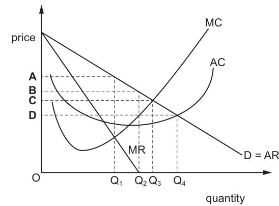
A government decides to use price controls to achieve allocative efficiency in a monopoly market.
Which price would need to be set to achieve allocative efficiency?
Options
A price A on Fig. 11.1
B price B on Fig. 11.1
C price C on Fig. 11.1
D price D on Fig. 11.1
Working
Allocative efficiency occurs where the price consumers pay (equal to average revenue, AR, and the marginal benefit of consumption) equals the marginal cost (MC) of producing the last unit. On the provided monopoly diagram, this is the point where the MC curve intersects the D = AR curve, which corresponds to price C.
Price A is the unregulated monopoly profit-maximising price (where MR = MC), price B is the normal profit price (where AR = AC), and price D is the productively efficient price (at the minimum of the AC curve). None of these satisfy the P = MC condition for allocative efficiency.
Answer
C
C
Background Concept
Allocative efficiency is a key welfare concept in economics that describes a situation where resources are allocated in a way that maximises total social surplus (the sum of consumer and producer surplus). The fundamental condition for allocative efficiency is that the marginal benefit (MB) of the last unit consumed equals the marginal cost (MC) of producing that unit. For a firm, the price consumers are willing to pay for a unit reflects the marginal benefit they receive from it, and average revenue (AR) is equal to the price charged. This means the allocative efficiency condition can be written as P = MC, or equivalently AR = MC.
In a perfectly competitive market, the profit-maximising equilibrium already satisfies P = MC, so the market outcome is allocatively efficient by default. However, in a monopoly market, the firm is a price-setter with a downward-sloping demand curve. It maximises profit by producing where marginal revenue (MR) equals MC, which results in a lower quantity and higher price than the allocatively efficient outcome. This creates a deadweight welfare loss, as some units for which MB > MC are not produced, reducing total social welfare.
Governments can intervene in monopoly markets to correct this market failure, for example by setting a price control (a maximum price) at the allocatively efficient level, forcing the monopoly to produce the socially optimal quantity.
Understanding the Question
This 1-mark multiple-choice question asks you to identify which of the four marked prices on the monopoly diagram (Fig. 11.1) would need to be set via a price control to achieve allocative efficiency. The diagram shows the standard curves for a monopoly: a downward-sloping demand curve (D) which is also the average revenue (AR) curve, a steeper downward-sloping marginal revenue (MR) curve, a U-shaped average cost (AC) curve, and an upward-sloping marginal cost (MC) curve. The four prices correspond to four key points on the diagram:
- Price A: intersection of MC and MR (unregulated monopoly profit-maximising point)
- Price B: intersection of AR and AC (normal profit, zero supernormal profit point)
- Price C: intersection of MC and AR (D)
- Price D: minimum point of the AC curve (productively efficient point)
The question tests two linked concepts: your knowledge of the condition for allocative efficiency, and your ability to apply that knowledge to interpret a monopoly diagram.
Approach
To answer this question, first recall the core condition for allocative efficiency: P = MC (or AR = MC, since AR = P for any firm). Next, locate the point on the diagram where the MC curve intersects the AR (D) curve, as this is the point where the allocative efficiency condition holds. The price corresponding to this intersection is the correct answer. You can eliminate the other options by identifying what each of the other price points represents, and confirming none of them satisfy the P = MC rule.
Step-by-Step Reasoning
- Confirm the allocative efficiency condition: Allocative efficiency requires that the marginal benefit to consumers of the last unit produced equals the marginal cost of producing that unit. Since the demand curve represents consumers' marginal benefit, and AR equals the price charged, this means we need to find the point where MC = AR (or MC = D).
- Locate the relevant intersection on the diagram: The MC curve is upward-sloping, and the D=AR curve is downward-sloping. Their intersection is at point C, so the price corresponding to this point is price C.
- Eliminate incorrect options:
- Price A is where MC = MR. This is the unregulated monopoly's profit-maximising outcome: the firm restricts output to Q1 to charge a higher price, creating deadweight loss, so this is not allocatively efficient.
- Price B is where AR = AC. At this price, the firm makes zero supernormal profit (only normal profit), but this is a firm-level outcome, not a social welfare outcome. MC is below AR here, so MB > MC, meaning more units should be produced to increase social welfare, so this is not allocatively efficient.
- Price D is at the minimum of the AC curve, which is the productively efficient point (the firm produces at the lowest possible average cost). However, at this price, MC is below AR, so MB > MC, meaning too little is being produced from a social perspective, so this is not allocatively efficient.
- Confirm the policy implication: If the government sets a maximum price (price control) at level C, the monopoly will be forced to supply the quantity where P = MC (Q3), which is the socially optimal quantity. This eliminates the deadweight loss from monopoly power and achieves allocative efficiency.
Key Takeaways
- The non-negotiable condition for allocative efficiency is P = MC (or AR = MC for a firm).
- Allocative efficiency is a social welfare concept, not a firm profitability concept: it depends on the equality of marginal benefit and marginal cost, not on whether the firm is making profit.
- Productive efficiency (minimum AC) and the monopoly profit-maximising outcome (MR = MC) are both distinct from allocative efficiency.
- Price controls are a common government intervention to correct monopoly market failure by forcing the firm to produce at the allocatively efficient output level.
Common Mistakes
- Confusing allocative efficiency with productive efficiency: Many students select price D (the minimum of the AC curve) because they associate efficiency with low costs. However, productive efficiency only refers to producing at the lowest average cost, not to producing the socially optimal quantity where MB = MC.
- Confusing the monopoly profit-maximising point with allocative efficiency: Students often select price A (where MR = MC) because it is the most prominent intersection on a monopoly diagram. However, this is the unregulated, inefficient monopoly outcome, not the socially efficient one.
- Confusing normal profit with social efficiency: Price B (where AR = AC) is the break-even point for the firm, but this does not mean the outcome is socially efficient, as MC is still below AR at this point.
Things to Be Careful About
- Always link the allocative efficiency condition to the relevant curves: MC (marginal cost) and AR/D (marginal benefit/price). Do not confuse MR with AR, as MR is not equal to price for a monopoly.
- Remember that allocative efficiency is about social welfare, not firm performance: a firm can make losses and still be allocatively efficient if P = MC, and a firm can make supernormal profit and be allocatively inefficient (as in the unregulated monopoly case).
- When interpreting monopoly diagrams, always label each intersection clearly to avoid mixing up the different outcomes (profit-maximising, normal profit, allocative efficiency, productive efficiency).
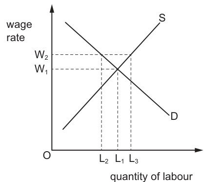
The diagram shows the supply of and the demand for workers in the car manufacturing industry.
A trade union successfully negotiates a wage increase from W1 to W2.
What is the likely impact on the level of employment?
Options
A fall from L1 to L2
B fall from L3 to L2
C rise from L1 to L3
D rise from L2 to L3
Reasoning
The labour market is initially in equilibrium at the intersection of the labour demand curve (D) and labour supply curve (S), where the wage rate is W1 and the level of employment is L1. When the trade union negotiates a higher wage W2 (above the equilibrium wage), the quantity of labour demanded by firms falls, as shown by the demand curve: at W2, the quantity of labour demanded is L2. Since employment is determined by the number of workers firms are willing and able to hire (quantity of labour demanded), not the number of workers willing to work (quantity of labour supplied, which is L3 at W2), the level of employment falls from L1 to L2.
Answer
A
A
Background Concept
The labour market for a specific industry (such as car manufacturing) is modelled using the standard supply and demand framework. The downward-sloping labour demand curve (D) reflects that firms will hire more workers only if the wage rate falls: this is because labour is a derived demand, derived from the demand for the final good (cars), and each additional worker adds marginal revenue product (MRP) to the firm. As more workers are hired, the MRP of labour falls (due to the law of diminishing marginal returns in the short run), so firms will only employ workers up to the point where the wage rate equals their MRP. The upward-sloping labour supply curve (S) reflects that higher wage rates attract more workers into the industry, or encourage existing workers to supply more hours of labour.
The equilibrium wage and employment are determined by the intersection of D and S: at wage W1, the quantity of labour demanded equals the quantity of labour supplied, so all workers who want to work at W1 can find a job, and all firms that want to hire at W1 can find workers. This equilibrium level of employment is L1.
Trade unions are organisations that represent workers in collective bargaining with employers. A key role of trade unions is to negotiate higher wages for their members. If a trade union is successful in negotiating a wage above the market equilibrium (such as W2 in this diagram), this creates a situation where the quantity of labour supplied exceeds the quantity of labour demanded at the new wage.
Understanding the Question
This question presents a labour market diagram for the car manufacturing industry, with an initial equilibrium at wage W1 and employment L1. A trade union has successfully negotiated a wage increase to W2. The question asks for the likely impact on the level of employment, with four options describing different changes in employment levels.
The question tests your ability to interpret a labour market supply and demand diagram, and apply the theory of wage determination to identify the effect of a higher wage on employment. It is a 1-mark multiple-choice question, so the correct answer is the one that matches the standard prediction of labour market theory for a wage set above equilibrium.
Approach
To solve this question, follow these steps:
- First, identify the initial equilibrium level of employment from the diagram: this is the quantity of labour at the intersection of D and S, which is L1, corresponding to wage W1.
- Next, find the quantity of labour demanded at the new higher wage W2: this is the value on the horizontal axis that aligns with W2 on the demand curve D, which is L2.
- Recall that employment in a labour market is equal to the quantity of labour actually hired by firms, which is the quantity of labour demanded, not the quantity of labour supplied. Even if more workers are willing to work at W2 (quantity supplied is L3), firms will only hire the number of workers they demand at that wage.
- Compare the new employment level (L2) to the original (L1) to find the direction and magnitude of the change: employment falls from L1 to L2.
- Match this outcome to the options: option A describes a fall from L1 to L2, so this is the correct answer.
Step-by-Step Reasoning
-
Interpret the initial equilibrium: The diagram shows the labour market for car manufacturing workers. The downward-sloping D curve is the demand for labour, and the upward-sloping S curve is the supply of labour. Their intersection is the market equilibrium, at wage W1 and employment level L1. This means that before the trade union negotiation, L1 workers are employed in the industry at a wage of W1.
-
Effect of the trade union wage increase: The trade union negotiates a higher wage W2, which is above the equilibrium wage W1. This is a mandatory higher wage for all workers in the industry, so firms cannot pay less than W2.
-
Find the quantity of labour demanded at W2: At the higher wage W2, firms will reduce the number of workers they hire, because the cost of each worker is now higher. To find how many workers firms will hire at W2, we look at the demand curve D: moving horizontally from W2 to the D curve, then down to the horizontal axis, gives the quantity of labour demanded, which is L2. This is because at W2, only workers whose MRP is at least W2 will be employed; workers with lower MRP are no longer worth employing at the higher wage.
-
Distinguish quantity demanded from quantity supplied: At W2, the quantity of labour supplied is L3 (found by moving from W2 to the S curve, then down to the horizontal axis). This means L3 workers are willing to work in the industry at W2, but firms only want to hire L2 workers. The difference (L3 - L2) is the number of workers who are unemployed as a result of the higher wage.
-
Determine the change in employment: The original employment level was L1, and the new employment level is L2. Since L2 is less than L1, employment falls from L1 to L2.
-
Eliminate incorrect options:
- Option B (fall from L3 to L2) is wrong because L3 is the quantity of labour supplied at W2, not the original employment level.
- Option C (rise from L1 to L3) is wrong because a higher wage reduces the quantity of labour demanded, so employment cannot rise, and L3 is the quantity supplied, not employment.
- Option D (rise from L2 to L3) is wrong for the same reason: employment falls, not rises, and L2 is the new employment level, not the original.
Key Takeaways
This question tests two core labour market concepts: (1) how equilibrium employment is determined by the intersection of labour demand and supply, and (2) the effect of a wage set above the equilibrium level on employment. The key takeaway is that employment is determined by the quantity of labour demanded, not the quantity supplied, when a wage is above equilibrium. Trade unions can push wages above the market-clearing level, but this comes at the cost of lower employment in the industry.
The skill of interpreting supply and demand diagrams for factor markets (like labour) is transferable to other markets, such as product markets or financial markets.
Common Mistakes
-
Confusing quantity of labour supplied with employment: The most common mistake is to select option B or C, which use L3 (the quantity of labour supplied at W2) as the employment level. Students often think that if more workers are willing to work at a higher wage, employment rises, but this ignores that employment depends on how many workers firms want to hire, not how many want to work.
-
Misidentifying the original equilibrium employment: Some students may misread the diagram and think the original employment is L2 or L3, leading them to select the wrong option. Always check that the original equilibrium is at the intersection of D and S, which corresponds to L1 here.
-
Assuming higher wages always increase employment: This is a common error if students confuse the supply side with the demand side of the labour market. While a higher wage increases the quantity of labour supplied, it reduces the quantity of labour demanded, and employment is determined by the lower of the two (quantity demanded) when the wage is above equilibrium.
-
Forgetting that the demand curve for labour is downward sloping: If a student thinks the demand curve for labour is upward sloping, they will incorrectly think that a higher wage leads to higher quantity demanded, and thus higher employment, leading them to select option C or D.
Things to Be Careful About
-
Always label curves correctly: In labour market diagrams, D is the demand for labour (downward sloping) and S is the supply of labour (upward sloping). Do not mix these up, as this will lead to reading the wrong quantity at W2.
-
Distinguish between quantity demanded and quantity supplied: When a wage is above equilibrium, there is excess supply of labour (unemployment), but employment is equal to the quantity demanded, not the quantity supplied.
-
Check the axis labels: The horizontal axis is quantity of labour, so the values L1, L2, L3 are employment levels, not wage rates.
-
Match the change to the question: The question asks for the impact on employment, not the number of unemployed workers or the quantity of labour supplied, so focus on the quantity of labour demanded at the new wage.
A firm buys new machinery which increases the marginal productivity of its workforce.
What will be the resulting impact on the market for labour?
Options
A a shift to the left in the demand curve for labour
B a shift to the right in the demand curve for labour
C a shift to the left in the supply curve for labour
D a shift to the right in the supply curve for labour
Answer
The demand for labour is a derived demand, based on the marginal revenue product (MRP) of labour. New machinery increases the marginal productivity of each worker, so the MRP of labour rises. At any given wage rate, the firm will now demand more labour. This is represented by a shift to the right in the demand curve for labour.
Answer
B
B
Background Concept
The demand for labour is a derived demand — it is not wanted for its own sake but for what it can produce. A firm hires workers because their output can be sold. The value of an additional worker to the firm is measured by the marginal revenue product (MRP) of labour, which is the extra revenue generated by employing one more unit of labour. MRP is calculated as:
MRP = marginal physical product (MPP) of labour × marginal revenue (MR) from selling that output.
In a perfectly competitive product market, MR equals the price of the good, so MRP = MPP × price. The firm's demand curve for labour is the downward-sloping MRP curve, because as more workers are hired, diminishing returns set in and MPP falls, reducing MRP.
Understanding the Question
The question states: "A firm buys new machinery which increases the marginal productivity of its workforce." This means the MPP of each worker rises — each worker can now produce more output per hour. The question asks for the resulting impact on the market for labour — specifically, which curve shifts and in which direction.
Key point: The machinery affects the productivity of labour, not the willingness of workers to supply their labour. Therefore, only the demand side of the labour market is affected. The supply curve for labour depends on factors such as wages, working conditions, preferences for leisure, and population — none of which are changed here.
Approach
- Identify that the demand for labour is derived from the MRP of labour.
- Recognise that an increase in marginal productivity raises the MRP at every level of employment.
- Conclude that the demand curve for labour shifts to the right (the firm wants to hire more workers at any given wage).
- Eliminate the options involving a shift in the supply curve, as the change is on the demand side.
Step-by-Step Reasoning
- Step 1: The firm's demand for labour is based on the MRP of labour. MRP = MPP × MR.
- Step 2: New machinery increases the MPP of labour — each worker produces more output.
- Step 3: Assuming the price of the output (MR) remains unchanged, the MRP of labour rises. For example, if a worker previously produced 10 units per hour worth $5 each (MRP = $50), after the machinery they might produce 15 units per hour worth $5 each (MRP = $75).
- Step 4: At the current wage rate, the firm now finds it profitable to hire more workers because the MRP exceeds the wage. The firm will increase its demand for labour.
- Step 5: This is represented graphically as a rightward shift of the demand curve for labour (from D1 to D2). At every wage rate, the quantity of labour demanded is higher.
- Step 6: The supply curve for labour is unaffected because the change is in productivity, not in workers' preferences or the wage they are willing to accept.
Thus, the correct answer is B: a shift to the right in the demand curve for labour.
Key Takeaways
- Labour demand is derived from the MRP of labour.
- Anything that increases the marginal productivity of labour (better technology, more capital, improved training) shifts the labour demand curve to the right.
- A change in productivity affects the demand side, not the supply side, of the labour market.
- Distinguish between a shift of the curve (caused by a change in a non-wage factor) and a movement along the curve (caused by a change in the wage rate).
Common Mistakes
- Confusing demand and supply: Some students might think that because workers become more productive, they will want to work more, shifting the supply curve. But supply depends on workers' decisions, not their productivity.
- Thinking of a movement along the curve: A change in the wage rate would cause a movement along the demand curve. Here, the wage is not mentioned; the change is in productivity, which shifts the entire curve.
- Assuming the machinery reduces labour demand: Some might think that machinery replaces labour, but the question explicitly says the machinery increases the marginal productivity of the workforce — it makes existing workers more productive, not redundant.
Things to Be Careful About
- Read the question carefully: "increases the marginal productivity of its workforce" — this is a positive productivity shock, not automation that replaces workers.
- Remember that the demand for labour is a derived demand — always link back to MRP.
- In multiple-choice questions, eliminate options that involve the wrong side of the market (supply vs demand) first, then choose the correct direction of shift.
The diagram represents the market for labour.
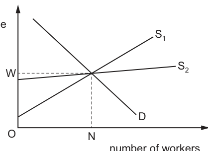
What would be the effect on transfer earnings and economic rent of a change in the supply curve from S1 to S2?
Options
| transfer earnings | economic rent | |
|---|---|---|
| A | fall | falls |
| B | fall | rises |
| C | rise | rises |
| D | rise | falls |
Transfer earnings are the minimum payment required to keep workers in their current employment, represented by the area under the supply curve up to the equilibrium quantity of labour (N). Economic rent is the excess payment above transfer earnings, represented by the area between the equilibrium wage (W) and the supply curve up to N. The supply curve S2 has a higher intercept on the wage axis than S1 and is flatter (more elastic), so it lies above S1 for all quantities of labour below N. This means the area under S2 up to N is larger than the area under S1, so transfer earnings rise. Since the equilibrium wage W and quantity N are unchanged, the total wage bill (W × N) is the same for both supply curves. As transfer earnings have risen, economic rent (total wage bill minus transfer earnings) falls.
Answer
D
D
Background Concept
Transfer earnings are the minimum remuneration a worker needs to supply their labour in a particular occupation, equal to the earnings they could earn in their next best alternative job. In a labour market diagram, transfer earnings are represented by the area under the labour supply curve up to the equilibrium quantity of labour employed, as the supply curve shows the minimum wage each worker requires to work.
Economic rent is any payment to a worker above their transfer earnings — it is the surplus earned due to factors such as scarcity of skills, monopsony power of employers, or institutional factors like trade unions. Graphically, economic rent is the area between the equilibrium wage rate and the labour supply curve up to the equilibrium quantity of labour.
The elasticity and position of the labour supply curve determine the relative size of transfer earnings and economic rent. A more inelastic (steeper) supply curve that starts lower on the wage axis means a smaller share of the total wage bill is transfer earnings and a larger share is economic rent, while a more elastic (flatter) supply curve that starts higher on the wage axis means a larger share is transfer earnings and a smaller share is economic rent. This is because the area under a higher, flatter curve up to a given quantity is larger than the area under a lower, steeper curve, while the area between a horizontal wage line and a higher, flatter curve is smaller than the area between the wage line and a lower, steeper curve.
Understanding the Question
The question provides a labour market diagram with a downward-sloping demand curve for labour (D) and two supply curves: S1 (relatively inelastic, steeper, starting at the origin) and S2 (more elastic, flatter, starting at a higher point on the wage axis). Both supply curves intersect the demand curve at the same point, resulting in the same equilibrium wage (W) and equilibrium quantity of workers (N). The question asks what happens to transfer earnings and economic rent when the supply curve shifts from S1 to S2.
This is a 1-mark multiple choice question that tests the candidate's ability to apply the definitions of transfer earnings and economic rent to a change in supply curve elasticity and position. The key point to note is that the two supply curves intersect demand at the same equilibrium, so the wage and employment levels do not change — only the distribution of the total wage bill between transfer earnings and economic rent changes.
Approach
To solve this question, first recall the graphical representation of transfer earnings and economic rent in a labour market. Then compare the relevant areas for S1 and S2 up to the equilibrium quantity N:
- Transfer earnings = area under the supply curve from 0 to N.
- Economic rent = area between the equilibrium wage line (W) and the supply curve from 0 to N.
Since S2 has a higher intercept on the wage axis and is flatter than S1, it lies above S1 for all quantities below N. This means the area under S2 is larger than the area under S1, while the area between W and S2 is smaller than the area between W and S1. We can also eliminate wrong options first: options A and C claim transfer earnings fall, which is incorrect, while option B claims economic rent rises, which is also incorrect, leaving D as the only possible answer.
Step-by-Step Reasoning
- First, confirm the equilibrium outcome: both S1 and S2 intersect the demand curve D at the same point, so the equilibrium wage (W) and equilibrium quantity of labour (N) are identical under both supply curves. This means the total wage bill (W × N) is unchanged by the shift from S1 to S2.
- Calculate the change in transfer earnings: Transfer earnings are the area under the labour supply curve up to N, representing the sum of the minimum wages required to employ each worker. The supply curve S2 starts at a higher wage on the vertical axis than S1 and is flatter (more elastic), so it lies above S1 for all quantities of labour between 0 and N. This means the area under S2 up to N is larger than the area under S1 up to N. When supply shifts from S1 to S2, transfer earnings rise.
- Calculate the change in economic rent: Economic rent is the total wage bill minus total transfer earnings, or equivalently the area between the equilibrium wage line (W) and the supply curve up to N. Since the total wage bill is unchanged and transfer earnings have risen, economic rent must fall. We can also confirm this graphically: the vertical distance between the horizontal wage line W and the supply curve is smaller for S2 than for S1 at every quantity below N, so the area between W and S2 is smaller than the area between W and S1.
- Match the outcome to the options: transfer earnings rise and economic rent falls, which corresponds to option D.
Key Takeaways
- Transfer earnings are the minimum total payment required to employ the equilibrium quantity of labour, represented by the area under the labour supply curve up to N.
- Economic rent is the surplus paid to workers above their transfer earnings, represented by the area between the equilibrium wage and the supply curve up to N.
- A more elastic labour supply curve with a higher wage intercept increases transfer earnings and reduces economic rent, ceteris paribus, because the flatter, higher supply curve has a larger area under it and a smaller area between it and the wage line.
- When supply curves intersect the demand curve at the same point, a change in supply elasticity and position does not affect equilibrium wage or employment, only the distribution of the total wage bill between transfer earnings and economic rent.
Common Mistakes
- Misreading the position of the supply curves: some students assume the steeper supply curve (S1) is above the flatter one (S2), leading them to incorrectly conclude transfer earnings fall and economic rent rises (option B). Always check the intercepts of the supply curves on the wage axis to determine which is higher at low quantities.
- Confusing the graphical representation of transfer earnings and economic rent: some students mix up which area corresponds to which concept, leading them to select the wrong option.
- Incorrectly assuming the supply shift changes equilibrium wage or employment: since both supply curves intersect demand at the same point, W and N are unchanged. Students who think the shift changes these values may miscalculate the areas.
- Misunderstanding the effect of supply elasticity and position: some students incorrectly believe a more elastic supply reduces transfer earnings, rather than increasing it, because they do not correctly compare the areas under the two supply curves.
Things to Be Careful About
- Always clearly identify the areas for transfer earnings and economic rent when analysing labour market diagrams: shading the area under the supply curve up to N as transfer earnings and the area between the wage line and supply curve as economic rent can help avoid confusion.
- Check the intercepts of the supply curves on the wage axis: in this question, S2 has a higher intercept than S1, so it lies above S1 for all quantities below N, leading to a larger area under S2.
- Check whether the supply curves intersect demand at the same point: in this question they do, so equilibrium outcomes are unchanged. If they intersected at different points, you would need to recalculate the equilibrium wage and employment first.
- For multiple choice questions, eliminate wrong options first: options A and C have transfer earnings falling, which is incorrect, and option B has economic rent rising, which is also incorrect, so D is the only valid answer.
Which combination of policies is most likely to increase the number of low-paid workers caught in the poverty trap?
Options
| individual’s tax-free allowance for income tax | proportion of all benefits that are means-tested | |
|---|---|---|
| A | decrease | increase |
| B | decrease | decrease |
| C | increase | increase |
| D | increase | unchanged |
Answer
The poverty trap occurs when a low-paid worker faces a high effective marginal tax rate: as earnings rise, income tax becomes payable and means-tested benefits are withdrawn, so net income rises very little or not at all.
- Decreasing the tax-free allowance means tax is paid on a larger portion of any extra earnings, raising the effective marginal tax rate.
- Increasing the proportion of benefits that are means-tested means more benefits are withdrawn as earnings rise, further raising the effective marginal tax rate.
Both changes worsen the poverty trap. Therefore the correct combination is A.
A
Background Concept
The poverty trap describes a situation where low-income workers face little or no net financial gain from increasing their work effort (e.g., working more hours or getting a higher-paying job). This happens because two things happen simultaneously when earnings rise:
- Income tax liability increases – the worker pays more tax on the extra income.
- Means-tested benefits are withdrawn – benefits that depend on income (e.g., housing benefit, tax credits) are reduced as earnings rise.
The combined effect is a high effective marginal tax rate – the proportion of each additional pound earned that is lost to tax and reduced benefits. If this rate is very high (sometimes over 100%), there is no financial incentive to work more, trapping the worker in low pay.
Understanding the Question
The question asks which combination of two policy changes is most likely to increase the number of low-paid workers caught in the poverty trap. The two policies are:
- A change in the individual's tax-free allowance for income tax (the amount of income you can earn before paying any tax).
- A change in the proportion of all benefits that are means-tested (the share of benefits that are withdrawn as income rises, rather than being universal or non-means-tested).
We need to decide whether each change should increase or decrease to make the poverty trap worse. The correct answer is the combination that raises the effective marginal tax rate the most.
Approach
- Understand how each policy change affects the effective marginal tax rate.
- For the tax-free allowance: a decrease means tax starts at a lower income, so more of any extra earnings is taxed – this raises the effective marginal tax rate.
- For means-tested benefits: a higher proportion means more benefits are withdrawn as income rises – this also raises the effective marginal tax rate.
- The combination that makes the trap worse is therefore: decrease the allowance AND increase the proportion of means-tested benefits. This is option A.
Step-by-Step Reasoning
-
Tax-free allowance: If the allowance is decreased, the worker starts paying income tax at a lower level of earnings. For example, if the allowance falls from $12,000 to $10,000, then on the next $2,000 of earnings the worker now pays tax that they previously did not. This directly increases the effective marginal tax rate on low earnings.
-
Means-tested benefits: If a larger proportion of benefits are means-tested, then a greater share of the worker's total benefit entitlement is withdrawn as earnings rise. For instance, if previously only 50% of benefits were means-tested, and now 80% are, then for each extra dollar earned, more benefit is lost. This also raises the effective marginal tax rate.
-
Combined effect: Both changes push in the same direction – they both increase the rate at which net income falls relative to gross earnings. This makes the poverty trap more severe, meaning more low-paid workers will find it financially unrewarding to increase their work effort.
-
Why the other options are wrong:
- B: Decreasing both the allowance and the proportion of means-tested benefits would have opposing effects – the allowance change worsens the trap, but the benefit change (fewer means-tested benefits) eases it. The net effect is ambiguous and not clearly the most likely to increase the trap.
- C: Increasing the allowance reduces the effective marginal tax rate (less tax on extra earnings), while increasing means-tested benefits raises it. Again, opposing effects.
- D: Increasing the allowance reduces the trap, and leaving the proportion of means-tested benefits unchanged does not worsen it. This combination would reduce the poverty trap, not increase it.
Key Takeaways
- The poverty trap is caused by a high effective marginal tax rate on low earnings, arising from the interaction of the tax system and means-tested benefits.
- Policies that increase the effective marginal tax rate (e.g., lowering the tax-free allowance, increasing the withdrawal rate of benefits) worsen the trap.
- Policies that decrease the effective marginal tax rate (e.g., raising the tax-free allowance, reducing means-testing) ease the trap.
- When evaluating policy combinations, consider whether each change pushes in the same direction or in opposite directions.
Common Mistakes
- Confusing the direction of the effect: Some students think that increasing the tax-free allowance helps the poor, so it must reduce the poverty trap – but the question asks which change increases the trap, so the opposite is needed.
- Ignoring the combined effect: Students may correctly identify one policy's effect but fail to consider the other, or assume that two changes that both seem 'pro-poor' must both reduce the trap, without checking the mechanism.
- Misunderstanding means-testing: Some think that more means-testing always helps target benefits to the poorest, but it also creates a higher withdrawal rate, which can worsen the poverty trap.
Things to Be Careful About
- The question asks for the combination most likely to increase the trap – not just any combination that might. Only option A has both changes pushing in the same direction to worsen the trap.
- Remember that the poverty trap is about incentives to increase earnings, not about the absolute level of income or benefits. A policy that gives more money to the poor can still worsen the trap if it raises the effective marginal tax rate.
- The effective marginal tax rate is the key concept – it is the sum of the marginal income tax rate and the marginal benefit withdrawal rate.
A website compares the prices of groceries.
Which function of money is illustrated by this?
Options
A medium of exchange
B standard of deferred payment
C store of value
D unit of account
Reasoning
Comparing prices requires a common measure of value. This is the function of money as a unit of account — it allows goods and services to be valued in a standard unit (e.g. dollars, pounds) so that prices can be compared directly.
Answer
D
D
Background Concept
Money serves four classic functions in an economy:
- Medium of exchange — money is accepted in exchange for goods and services, eliminating the need for a double coincidence of wants that exists under barter.
- Unit of account — money provides a standard numerical unit of measurement for the value of goods, services, assets, and debts. It allows prices to be quoted and compared.
- Store of value — money can be saved and used for future purchases, provided its purchasing power is reasonably stable over time.
- Standard of deferred payment — money is used to settle debts that are payable in the future, enabling credit transactions.
Understanding the Question
The question describes a website that compares the prices of groceries. The key action is "comparing prices" — this involves expressing the value of different groceries in a common monetary unit (e.g., $2.50 for milk, $1.80 for bread). The question asks which function of money is illustrated by this activity.
Approach
Read the scenario carefully: the website is not facilitating a purchase (which would be medium of exchange), not enabling saving (store of value), and not settling a future debt (standard of deferred payment). It is simply allowing consumers to see and compare the monetary values of different items. This directly matches the unit of account function.
Step-by-Step Reasoning
- Identify the action: "compares the prices of groceries."
- Consider each function:
- Medium of exchange (A): This would involve using money to actually buy the groceries — the website is not a payment platform, it is a comparison tool.
- Standard of deferred payment (B): This relates to using money to settle debts over time — not relevant to a price comparison site.
- Store of value (C): This involves holding money to preserve purchasing power for future use — the website does not store money.
- Unit of account (D): This is the function of measuring and comparing value. The website uses money as a common denominator to list and compare prices, which is exactly what a unit of account does.
- Therefore, the correct answer is D.
Key Takeaways
- The four functions of money are distinct and can be tested through real-world examples.
- "Comparing prices" is a classic illustration of the unit of account function.
- Be careful not to confuse "comparing prices" with "buying goods" — the latter would be medium of exchange.
Common Mistakes
- Choosing medium of exchange because the website involves money and groceries. The website does not facilitate the actual exchange; it only displays prices.
- Choosing store of value because the website might help you decide where to save money. The function illustrated is about measuring value, not storing it.
- Overthinking the scenario — the question is straightforward and tests a single concept.
Things to Be Careful About
- Read the scenario precisely: the action is "compares prices," not "buys groceries."
- Remember that a single transaction can involve multiple functions, but the question asks which function is illustrated by the specific action described.
Two statements about the types of unemployment are shown.
1 You will get unemployment if you pay people not to work, and tax them when they do.
2 An individual is actively seeking work but due to negative economic growth cannot find employment.
Which row best describes the two types of unemployment in these statements?
Options
| 1 | 2 | |
|---|---|---|
| A | cyclical | structural |
| B | voluntary | frictional |
| C | structural | cyclical |
| D | voluntary | involuntary |
Reasoning
Statement 1 describes a situation where individuals choose not to work because of high benefits relative to wages, which is voluntary unemployment. Statement 2 describes an individual actively seeking work but unable to find it due to negative economic growth, which is involuntary unemployment, specifically cyclical. Option D correctly identifies statement 1 as voluntary and statement 2 as involuntary.
Answer
D
D
Background Concept
Unemployment can be classified into several types. Voluntary unemployment occurs when individuals choose not to work at the prevailing wage rate, often due to generous welfare benefits, high marginal tax rates, or personal preferences. Involuntary unemployment occurs when individuals are willing and able to work at the going wage but cannot find jobs. Cyclical unemployment is a type of involuntary unemployment caused by a downturn in the business cycle (negative economic growth). Structural unemployment arises from a mismatch between workers' skills and job requirements, or geographic immobility. Frictional unemployment is short-term unemployment during the process of moving between jobs.
Understanding the Question
The question presents two statements and asks which row best describes the types of unemployment. Statement 1: "You will get unemployment if you pay people not to work, and tax them when they do." This implies that if benefits are high and taxes on work are high, people may choose not to work — this is a classic example of voluntary unemployment. Statement 2: "An individual is actively seeking work but due to negative economic growth cannot find employment." This describes a person who wants to work but cannot because of recession — this is involuntary unemployment (cyclical). The answer choices mix terms: voluntary, involuntary, cyclical, structural, frictional. We need to select the row that correctly labels both statements.
Approach
First, identify the correct type for each statement independently. Then, check each option to see which row matches. Option A: 1 = cyclical, 2 = structural — incorrect. Option B: 1 = voluntary, 2 = frictional — frictional is not due to negative economic growth. Option C: 1 = structural, 2 = cyclical — structural for statement 1 is wrong. Option D: 1 = voluntary, 2 = involuntary — correct. Thus D is the answer.
Step-by-Step Reasoning
-
Analyze statement 1: "You will get unemployment if you pay people not to work, and tax them when they do." This is a classic description of the unemployment trap: when welfare benefits are high and taxes on income are high, the net gain from working is low, so some individuals choose not to work. This is voluntary unemployment because the decision is based on choice. It is not structural (which is about mismatch of skills) nor cyclical (which is due to demand deficiency) nor frictional (temporary). So statement 1 corresponds to voluntary unemployment.
-
Analyze statement 2: "An individual is actively seeking work but due to negative economic growth cannot find employment." Negative economic growth means the economy is in a recession, leading to falling aggregate demand. This causes demand-deficient or cyclical unemployment. The individual is willing and able to work but cannot find a job — this is involuntary unemployment. Frictional unemployment would be short-term and not directly caused by negative growth. Structural unemployment would be due to changes in the structure of the economy, not necessarily negative growth. So statement 2 is involuntary (cyclical).
-
Now examine each option:
- Option A: 1 = cyclical, 2 = structural. Statement 1 is not cyclical, so A is wrong.
- Option B: 1 = voluntary, 2 = frictional. Statement 2 is not frictional, so B is wrong.
- Option C: 1 = structural, 2 = cyclical. Statement 1 is not structural, so C is wrong.
- Option D: 1 = voluntary, 2 = involuntary. Both match, so D is correct.
-
Therefore, the correct answer is D.
Key Takeaways
- Understand the definitions of different types of unemployment: voluntary, involuntary, cyclical, structural, frictional.
- Be able to identify which type is described by a given scenario.
- Voluntary unemployment stems from choices influenced by incentives (benefits, taxes).
- Involuntary unemployment arises from macroeconomic conditions (cyclical) or structural mismatches.
Common Mistakes
- Confusing voluntary with structural: The first statement is about incentives, not about skill mismatch. Some students might incorrectly think it is structural because it involves government policy, but structural unemployment is about mismatch of skills/location.
- Confusing cyclical with structural: The second statement mentions negative economic growth, which is a clear sign of cyclical unemployment, not structural. Some might think any unemployment due to recession is structural, but that's wrong.
- Mixing up frictional and voluntary: Frictional is short-term and usually involves people between jobs, not choosing not to work due to benefits.
Things to Be Careful About
- Read each statement carefully: note the key phrases "pay people not to work" and "tax them when they do" signal voluntary unemployment. "Negative economic growth" signals cyclical/involuntary.
- Remember that cyclical unemployment is a subset of involuntary unemployment. The question allows "involuntary" as the broader category, which is correct here.
- Do not overthink: the simplest interpretation is often correct.
A government decides to cut the rate of interest in order to stimulate aggregate demand and increase employment.
Why might this policy not work in a recession?
Options
A Business confidence is low.
B It leads to deflation.
C It leads to an appreciation in the exchange rate.
D It leads to a decrease in the money supply.
Reasoning
In a recession, business confidence is low. Firms are pessimistic about future demand and are reluctant to borrow and invest even if interest rates fall. The lower cost of borrowing does not translate into higher investment or consumption because the transmission mechanism is blocked by weak confidence. This is the liquidity trap scenario: the policy fails to stimulate aggregate demand.
Answer
A
A
Background Concept
Monetary policy works through a transmission mechanism: a cut in the central bank's policy rate reduces commercial bank lending rates, which lowers the cost of borrowing for firms and households. Lower borrowing costs should, in theory, stimulate investment (firms borrow to expand) and consumption (households borrow for durables or mortgages), thereby increasing aggregate demand (AD). However, this mechanism depends on the willingness of agents to borrow. In a recession, confidence is typically very low — firms see falling sales and uncertain future demand, and households fear unemployment. Even at very low interest rates, borrowing may not rise because the expected return on investment is negative or too uncertain. This is the essence of the 'liquidity trap' described by Keynes: monetary policy becomes ineffective because the demand for money becomes infinitely elastic at a very low interest rate, and the policy fails to boost spending.
Understanding the Question
The question asks why a cut in the interest rate might fail to stimulate AD and increase employment during a recession. The four options present possible reasons. The correct one is the one that directly explains why the transmission mechanism breaks down. Option A (low business confidence) is the classic Keynesian explanation. Option B (it leads to deflation) is incorrect because lower interest rates are expansionary and tend to raise inflation, not cause deflation. Option C (it leads to an appreciation in the exchange rate) is the opposite of what usually happens — lower interest rates tend to cause depreciation (capital outflows reduce demand for the currency). Option D (it leads to a decrease in the money supply) is wrong because cutting the interest rate is an expansionary monetary policy that increases the money supply (or at least does not decrease it).
Approach
Identify the key reason why the transmission mechanism of monetary policy fails in a recession. The correct answer is the one that explains why lower borrowing costs do not translate into higher spending. Eliminate the other three options by checking whether they are plausible consequences of an interest rate cut and whether they would block the policy's effectiveness.
Step-by-Step Reasoning
-
Understand the policy: A cut in the interest rate is an expansionary monetary policy. It aims to lower the cost of borrowing, encouraging firms to invest and households to consume, thereby shifting AD rightwards and raising employment.
-
Identify the failure mechanism: In a recession, the problem is not the cost of borrowing but the willingness to borrow. Firms are pessimistic about future sales and profits. Even if loans are cheap, they see no profitable investment opportunities. Households, worried about job security, may prefer to save rather than spend. This is the 'liquidity trap' — the demand for money is highly elastic, and the interest rate cut does not stimulate spending.
-
Evaluate each option:
- A: Business confidence is low. This is correct. Low confidence means firms do not respond to lower interest rates by investing. The transmission mechanism is blocked.
- B: It leads to deflation. This is false. Expansionary monetary policy is inflationary, not deflationary. A cut in interest rates tends to raise the price level, not lower it.
- C: It leads to an appreciation in the exchange rate. This is false. Lower interest rates make domestic assets less attractive to foreign investors, reducing demand for the currency and causing depreciation (or at least preventing appreciation).
- D: It leads to a decrease in the money supply. This is false. Cutting interest rates is typically achieved by increasing the money supply (e.g., through open market purchases). The money supply rises, not falls.
-
Conclusion: The only option that correctly explains why the policy might not work is A.
Key Takeaways
- The transmission mechanism of monetary policy depends on the responsiveness of borrowing and spending to changes in interest rates.
- In a recession, low business confidence can render interest rate cuts ineffective — a phenomenon known as the liquidity trap.
- Always consider the state of confidence and expectations when evaluating the effectiveness of monetary policy.
- Be careful not to confuse the effects of monetary policy: lower interest rates are expansionary (inflationary, depreciating currency, increasing money supply), not contractionary.
Common Mistakes
- Choosing option C (appreciation) because students sometimes think lower interest rates attract foreign capital. In fact, lower rates make domestic assets less attractive, leading to depreciation.
- Choosing option D (decrease in money supply) because students confuse the direction of policy: cutting rates is expansionary and increases the money supply.
- Choosing option B (deflation) because students think lower interest rates reduce inflation. In reality, lower rates stimulate demand and raise inflation.
Things to Be Careful About
- Read the question carefully: it asks why the policy might NOT work. The correct answer must explain a failure of the transmission mechanism, not a side effect that would actually help the policy.
- Remember that in a recession, the problem is often a lack of demand, not the cost of credit. The policy fails because the demand for loans is interest-inelastic when confidence is low.
- Distinguish between the intended effect of a policy and the conditions that prevent it from working.
Households in an economy change their consumption behaviour causing the consumption curve to shift from C1 to C2.
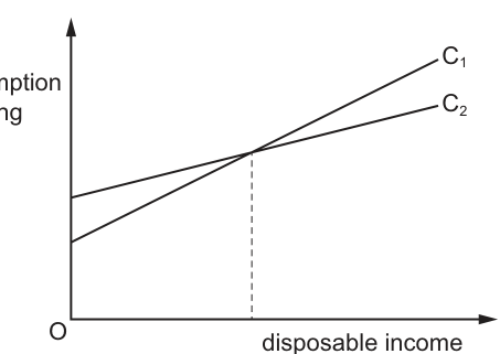
What has happened to autonomous consumption and the marginal propensity to consume?
Options
| autonomous consumption | marginal propensity to consume | |
|---|---|---|
| A | decreased | decreased |
| B | decreased | increased |
| C | increased | decreased |
| D | increased | increased |
Working
Autonomous consumption is the level of consumption when disposable income is zero, represented by the vertical intercept of the consumption function. The marginal propensity to consume (MPC) is the change in consumption for a given change in disposable income, equal to the slope of the consumption function.
In the diagram, the shift from C1 to C2 lowers the vertical intercept, so autonomous consumption has decreased. C2 has a flatter slope than C1, so the MPC has decreased.
Answer
C
C
Background Concept
The consumption function is a core component of aggregate demand, modelling the relationship between total household consumption spending and disposable income (income after taxes and transfer payments). It is typically expressed as C = a + bY, where:
- a is autonomous consumption: the amount households spend even when disposable income (Y) is zero, funded by past savings or borrowing. This is the vertical intercept of the consumption function on a graph with consumption on the vertical axis and disposable income on the horizontal axis.
- b is the marginal propensity to consume (MPC): the fraction of each additional unit of disposable income that households spend on consumption. It is calculated as MPC = ΔC / ΔY (change in consumption divided by change in disposable income), which equals the slope (gradient) of the consumption function line, as slope is defined as rise over run (ΔC/ΔY).
The MPC is always positive and less than 1, because households spend part but not all of any extra income, saving the remainder. The marginal propensity to save (MPS) is equal to 1 - MPC, as all income is either consumed or saved.
Understanding the Question
The question provides a diagram of two consumption functions, C1 and C2, showing that households have changed their consumption behaviour, shifting the consumption curve from C1 to C2. It asks what has happened to two specific parameters of the consumption function: autonomous consumption (the intercept a) and the marginal propensity to consume (the slope b). This is a 1-mark multiple-choice question, so it requires only correct identification of these two values from the diagram, with no further calculation or evaluation needed.
Approach
To answer this, we first recall what each of the two terms represents in the context of the consumption function diagram:
- Autonomous consumption corresponds to the point where the consumption line meets the vertical (consumption) axis, i.e., the value of C when disposable income is 0.
- MPC corresponds to the steepness (slope) of the consumption line: a steeper line means a higher MPC, a flatter line means a lower MPC.
We then compare the positions and slopes of C1 and C2 in the diagram to see how each parameter has changed.
Step-by-Step Reasoning
- First, assess autonomous consumption: Look at where each line crosses the vertical (consumption) axis. C1 has a higher vertical intercept than C2, meaning that at a disposable income of 0, consumption was higher under C1 than under C2. This means autonomous consumption has decreased when moving from C1 to C2.
- Next, assess the MPC: Look at the slope of each line. C1 is steeper than C2. A steeper slope means that for any given increase in disposable income, consumption increases by more under C1 than under C2. Since MPC measures how much consumption rises per unit rise in income, the flatter slope of C2 means the MPC has decreased.
- Match these findings to the options: Autonomous consumption decreased, MPC decreased, which corresponds to option C.
Key Takeaways
- The consumption function is written as C = a + bY, where a is autonomous consumption (vertical intercept) and b is MPC (slope).
- Changes in autonomous consumption shift the entire consumption function up or down without changing its slope.
- Changes in the MPC change the slope of the consumption function, without necessarily shifting the intercept (though both can change at once, as in this question).
- Always match the diagram feature to the economic concept: intercept = autonomous value, slope = marginal propensity.
Common Mistakes
- Confusing the intercept and slope: Some students mix up which part of the consumption function represents autonomous consumption and which represents MPC, leading them to select the wrong option.
- Misreading the slope: A flatter line means a lower MPC, not higher — students may incorrectly think a steeper line is a lower MPC, or vice versa.
- Ignoring the direction of the shift: It is easy to misread which line is C1 and which is C2, leading to the wrong conclusion about whether the values increased or decreased.
Things to Be Careful About
- Always check the axis labels: The vertical axis is consumption, horizontal is disposable income, so the intercept is consumption at zero income, not the other way around.
- Remember that MPC is always between 0 and 1, so any slope of the consumption function (which is upward sloping) will correspond to an MPC in that range, but a flatter slope still means a lower MPC than a steeper one.
- For multiple-choice questions, eliminate wrong options first: here, options A and B state autonomous consumption decreased (correct), but A says MPC decreased (correct) while B says MPC increased (incorrect), so B is eliminated. Options C and D state MPC decreased (correct), but D says autonomous consumption increased (incorrect), so D is eliminated, leaving C as the only correct option.
How would decreasing interest rates be most likely to reduce unemployment?
Options
A by decreasing the borrowing costs of business
B by decreasing the government’s budget deficit
C by increasing the foreign exchange rate of the currency
D by increasing the opportunity cost of spending
Reasoning
A decrease in interest rates reduces the cost of borrowing for firms. Lower borrowing costs encourage firms to take out loans to finance investment in capital equipment and expansion. Increased investment raises aggregate demand (AD) and, in the short run when the economy is below full capacity, firms increase output and hire more workers, reducing unemployment. This is the standard transmission mechanism of expansionary monetary policy.
Option B is incorrect because a lower interest rate does not directly reduce the government's budget deficit; it may even increase it if the government's debt servicing costs fall but tax revenues also fall. Option C is incorrect because lower interest rates typically cause the currency to depreciate (capital outflows seeking higher returns elsewhere), not appreciate. Option D is incorrect because a lower interest rate reduces the opportunity cost of spending (the interest forgone by not saving), which would increase spending, not reduce unemployment through the channel described.
Answer
A
A
Background Concept
Monetary policy is a demand-side policy used by central banks to influence aggregate demand (AD) and, through it, macroeconomic objectives such as price stability, growth, and employment. The main instrument is the policy interest rate (e.g., the Bank Rate or Federal Funds Rate). A decrease in the policy rate is expansionary: it aims to stimulate spending and output.
The transmission mechanism works through several channels:
- Cost of borrowing channel: Lower interest rates reduce the cost of loans for firms (investment) and households (consumption of durables).
- Wealth channel: Lower rates may raise asset prices (shares, bonds, property), increasing household wealth and confidence, boosting consumption.
- Exchange rate channel: Lower rates make domestic assets less attractive to foreign investors, causing the currency to depreciate, which makes exports cheaper and imports dearer, boosting net exports.
- Cash-flow channel: Lower rates reduce debt-servicing costs for borrowers with variable-rate loans, freeing up disposable income for other spending.
Unemployment is reduced when AD rises and firms respond by increasing production and hiring. This is most effective when the economy is operating below full capacity (a negative output gap).
Understanding the Question
The question asks which of four options describes the most likely mechanism by which a decrease in interest rates reduces unemployment. It is a single-best-answer multiple-choice question. The key is to identify the direct, first-round causal link in the transmission mechanism. Options B, C, and D describe effects that are either incorrect, indirect, or opposite to what actually happens.
Approach
- Recall the standard transmission mechanism of expansionary monetary policy.
- For each option, ask: "Does this describe a direct, plausible causal link from lower interest rates to lower unemployment?"
- Option A is the textbook first step: lower rates -> cheaper borrowing -> more investment -> higher AD -> more output -> more jobs.
- Test the others: B (budget deficit) is not directly affected by interest rates in a simple way; C (exchange rate) moves in the opposite direction; D (opportunity cost) moves in the opposite direction.
Step-by-Step Reasoning
Option A: "by decreasing the borrowing costs of business"
- A decrease in the central bank's policy rate leads commercial banks to lower their lending rates (the base rate plus a margin).
- Firms face a lower cost of borrowing for investment projects (new machinery, factories, technology).
- Some projects that were previously unprofitable (because the expected rate of return was below the cost of borrowing) now become viable.
- Firms increase investment spending (I), a component of AD.
- Higher AD, if the economy has spare capacity, leads firms to increase output (Y).
- To produce more output, firms hire more workers, reducing unemployment.
- This is a direct, well-established causal chain. It is the most likely mechanism.
Option B: "by decreasing the government's budget deficit"
- A lower interest rate reduces the government's debt-servicing costs on its outstanding debt (if it has variable-rate debt or refinances at lower rates). This could reduce the deficit slightly.
- However, a lower deficit means the government is borrowing less, which is contractionary (reduces AD) — the opposite of what is needed to reduce unemployment.
- Moreover, the primary effect of lower rates on unemployment runs through private-sector spending, not the government's budget position. This option describes a secondary, ambiguous, and likely counterproductive effect.
Option C: "by increasing the foreign exchange rate of the currency"
- Lower interest rates make domestic assets less attractive to foreign investors (they can get higher returns elsewhere). This leads to capital outflows and a depreciation (fall) of the exchange rate, not an appreciation (rise).
- A depreciation would boost net exports (X-M) and AD, which could reduce unemployment. But the option says "increasing the foreign exchange rate" (appreciation), which is the opposite of what actually happens. So this option is factually incorrect.
Option D: "by increasing the opportunity cost of spending"
- The opportunity cost of spending is the interest income forgone by not saving. A lower interest rate reduces this opportunity cost, making spending more attractive relative to saving.
- This would increase consumption (C) and AD, which could reduce unemployment. However, the option says "increasing the opportunity cost", which is the opposite of what happens. So this option is also factually incorrect.
Therefore, only Option A describes a correct and direct causal mechanism.
Key Takeaways
- The transmission mechanism of monetary policy is a core concept: interest rate -> borrowing costs -> investment/consumption -> AD -> output -> employment.
- In multiple-choice questions, test each option against the standard theory. Look for options that describe the opposite effect (C and D) or an irrelevant/contradictory effect (B).
- "Most likely" means the most direct and well-established causal link, not a secondary or ambiguous one.
Common Mistakes
- Confusing the exchange rate effect: Many students think lower rates strengthen the currency (because they associate higher rates with a stronger currency). The opposite is true: lower rates weaken the currency.
- Confusing the opportunity cost effect: Lower rates make spending cheaper relative to saving, so the opportunity cost of spending falls, not rises.
- Overthinking the budget deficit: Students may know that lower rates reduce government debt interest, but they forget that a smaller deficit is contractionary, not expansionary. The question asks about reducing unemployment, which requires expansionary pressure.
Things to Be Careful About
- Read each option carefully. Options C and D contain the words "increasing" — check whether the actual effect is an increase or a decrease.
- Remember that the most likely mechanism is the one that is most direct and has the strongest theoretical support. Option A is the textbook answer.
- Do not confuse the effect on the exchange rate (depreciation) with the effect on net exports (increase). The option describes the exchange rate itself, not the trade effect.
The diagram shows a curve representing the relationship between a country’s unemployment rate and its inflation rate.
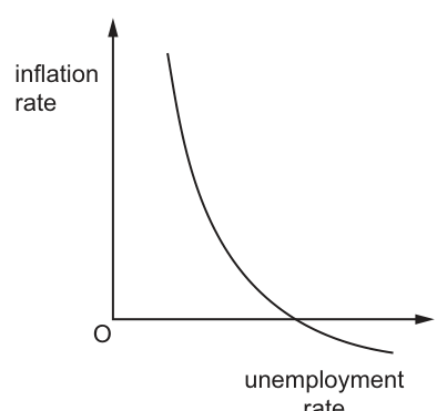
Why is it likely that this curve only applies in the short run?
Options
A Any attempt to reduce unemployment will increase inflation.
B Increased inflation actually increases unemployment.
C Increased inflation leads to expectations of further inflation.
D Increased inflation reduces real wage rates, which increases the demand for labour.
Working
The diagram shows a downward-sloping short-run Phillips curve (SRPC), which depicts an inverse relationship between inflation and unemployment in the short run. This trade-off only holds in the short run because, over time, workers and firms adjust their inflation expectations: if inflation rises, people come to expect further inflation, leading them to renegotiate higher nominal wages to preserve real wages. This shifts the SRPC upwards, eliminating the unemployment-inflation trade-off in the long run, where the Phillips curve is vertical at the natural rate of unemployment.
Option A describes the short-run trade-off itself, not the reason it is temporary. Option B is incorrect as the short-run relationship is inverse, not positive. Option D describes the short-run mechanism that creates the downward slope, but not why the relationship does not hold in the long run. Option C correctly identifies the role of adjusting inflation expectations in making the curve short-run only.
Answer
C
C
Background Concept
The Phillips curve illustrates the relationship between a country's inflation rate and its unemployment rate. The original short-run Phillips curve (SRPC) is downward-sloping and convex to the origin, showing an inverse relationship: lower unemployment is associated with higher inflation, and vice versa, in the short run. This relationship arises because when aggregate demand rises, firms increase output and hire more workers, reducing unemployment, but higher demand also pushes up prices, increasing inflation. In the long run, however, the Phillips curve is vertical at the natural rate of unemployment (the rate consistent with stable inflation), meaning there is no permanent trade-off between inflation and unemployment. This long-run result comes from the role of inflation expectations: over time, workers and firms adjust their expectations of future inflation to match actual inflation, eliminating the short-run trade-off.
Understanding the Question
The question presents a downward-sloping Phillips curve (the short-run version) and asks why this curve only applies in the short run. The task is to select the option that explains why the inverse inflation-unemployment relationship is temporary, not permanent. The key is to distinguish between the short-run mechanism that creates the downward slope, and the reason that mechanism breaks down over time.
Approach
First, recall the core difference between the short-run and long-run Phillips curve: the short-run trade-off exists because inflation expectations are static (adaptive) in the short run, but adjust over time. Then evaluate each option against this distinction:
- Eliminate options that describe the short-run trade-off itself, rather than why it is temporary.
- Eliminate options that describe the short-run mechanism of the curve, rather than the reason it does not hold in the long run.
- Select the option that links the short-run relationship to the adjustment of expectations over time.
Step-by-Step Reasoning
- First, identify what the diagram shows: it is the short-run Phillips curve (SRPC), which plots an inverse relationship between inflation (y-axis) and unemployment (x-axis).
- Evaluate Option A: "Any attempt to reduce unemployment will increase inflation." This is a description of the short-run trade-off that the SRPC depicts, but it does not explain why this trade-off only exists in the short run. In the long run, attempts to reduce unemployment below the natural rate do not lead to permanently higher inflation, so this is not the correct reason.
- Evaluate Option B: "Increased inflation actually increases unemployment." This is factually incorrect for the short-run Phillips curve, which shows an inverse (negative) relationship between the two variables, not a positive one. This is wrong.
- Evaluate Option D: "Increased inflation reduces real wage rates, which increases the demand for labour." This is the short-run mechanism that creates the downward slope of the SRPC: when inflation rises unexpectedly, nominal wages are sticky in the short run, so real wages fall, making labour cheaper for firms, who hire more workers, reducing unemployment. However, this mechanism only works in the short run because workers will eventually adjust their nominal wage demands to match higher inflation, restoring real wages to their original level. This option describes why the curve is downward-sloping, not why it is only short-run, so it is incorrect.
- Evaluate Option C: "Increased inflation leads to expectations of further inflation." This is the correct reason. In the short run, workers and firms have adaptive expectations: they do not immediately expect inflation to remain high, so the short-run trade-off holds. But over time, as inflation persists, people adjust their inflation expectations upwards. Workers will demand higher nominal wages to protect their real wages, which increases firms' costs, shifting the SRPC upwards. This means that any attempt to keep unemployment below the natural rate via higher inflation will only work temporarily, as expectations adjust, eliminating the trade-off in the long run. This is exactly why the SRPC only applies in the short run.
Key Takeaways
- The short-run Phillips curve shows a temporary inverse trade-off between inflation and unemployment, driven by sticky nominal wages and static inflation expectations in the short run.
- The long-run Phillips curve is vertical at the natural rate of unemployment, because inflation expectations adjust over time, eliminating the short-run trade-off.
- When answering questions about the time horizon of the Phillips curve, always distinguish between the short-run mechanism (sticky wages, static expectations) and the long-run adjustment (changing inflation expectations).
Common Mistakes
- Confusing the short-run trade-off (Option A) with the reason it is temporary: many students select A because it describes what the SRPC shows, but it does not explain why the curve does not apply in the long run.
- Selecting the short-run mechanism (Option D) instead of the reason for its temporary nature: D explains why the curve slopes downward, not why it is only valid short run.
- Forgetting that the long-run adjustment is driven by changing inflation expectations, which is the core of the expectations-augmented Phillips curve theory.
Things to Be Careful About
- Always read the question carefully: it asks why the curve only applies in the short run, not what the curve shows or why it slopes downward.
- Distinguish between positive statements (what is) and causal explanations (why something is the case): Option A is a positive statement about the short-run relationship, not a causal explanation for its temporary nature.
- Remember that the long-run Phillips curve is vertical because expectations adjust, so any option that does not mention expectations or adjustment over time is unlikely to be correct.
What is the most likely result of a period of negative actual growth?
Options
A an increase in the surplus of the financial account of the balance of payments
B an increase in the deficit of the current account of the balance of payments
C an increase in the rate of inflation
D an increase in the rate of unemployment
Negative actual growth means that the economy's real output is contracting – a recession. As output falls, firms reduce their workforce, so the demand for labour falls. The most direct and certain result is therefore an increase in the rate of unemployment. Inflation typically falls (not rises) during a recession. The current account deficit may widen if imports fall less than exports, but this is less predictable. The financial account surplus is not a direct or likely result.
Answer
D
D
Background Concept
Negative actual growth refers to a fall in the real gross domestic product (GDP) of an economy over a period, typically a quarter or a year. This is the defining feature of a recession or a contraction phase of the business cycle. When real output falls, the demand for labour – a derived demand – falls because fewer goods and services are being produced. Firms respond by reducing their workforce, which raises the unemployment rate. This is known as demand-deficient or cyclical unemployment.
Understanding the Question
The question asks for the most likely result of a period of negative actual growth, among four options. It tests your understanding of the typical short-run macroeconomic consequences of a recession. The four options cover the balance of payments financial account, the current account deficit, inflation, and unemployment. The key is “most likely” – which one is a near-certain, direct consequence?
Approach
Think through each option logically, using the chain of reasoning from falling output to each variable.
- Unemployment: falling output → lower demand for labour → fewer workers needed → higher unemployment. This is direct and occurs in every recession.
- Inflation: recessions reduce aggregate demand, which puts downward pressure on prices, so inflation tends to fall, not rise. Option C is wrong.
- Current account deficit: a recession reduces incomes, so imports typically fall, which may improve the current account (reduce a deficit or increase a surplus). A worsening deficit is unlikely. Option B is therefore wrong.
- Financial account surplus: the financial account records capital flows. A recession might affect investor confidence and capital flows, but the effect is ambiguous. A surplus is not a typical direct result. Option A is wrong.
Step-by-Step Reasoning
- Negative actual growth → real GDP is falling.
- Falling output → firms produce fewer goods and services → less labour is needed → demand for labour falls.
- Lower demand for labour → at given wage rates, there is an excess supply of labour → unemployment rises.
- This is the most direct and robust causal link.
For inflation: falling AD → downward pressure on the general price level → disinflation or even deflation, not rising inflation.
For the current account: falling income → lower spending on imports → net exports (X – M) rises → current account improves, not worsens.
For the financial account: capital flows depend on interest rates, confidence, and expectations; no consistent direct effect.
Therefore, the only certain and most likely result is an increase in the rate of unemployment.
Key Takeaways
- Negative actual growth = recession = falling real GDP.
- A recession raises unemployment through reduced demand for labour.
- Other macroeconomic variables like inflation, the current account, and capital flows have less predictable or opposite-direction changes.
- Focus on the most direct chain of causation when asked for “most likely”.
Common Mistakes
- Confusing negative actual growth with negative potential growth or deflation.
- Thinking that inflation always rises during a recession (it usually falls).
- Assuming that a recession always worsens the current account deficit – in fact, falling imports tend to improve it.
- Overcomplicating the financial account effects; remember, the question asks for the most likely, not a possible outcome.
Things to Be Careful About
- “Actual growth” refers to the change in real GDP, not potential growth.
- The link from output to unemployment is strong but can have lags; nonetheless, it is the most direct.
- Read each option carefully – distinguish between the current account and the financial account of the balance of payments.
An economy experiences falling incomes and rising unemployment. The central bank decides to reduce the rate of interest to stimulate economic activity.
When would such a policy be most likely to succeed?
Options
A when spending by consumers on goods and services is income elastic
B when spending by firms on capital goods is interest rate elastic
C when the leakage on additional national income is high
D when the overseas demand for exports is price inelastic
Reasoning
A reduction in the rate of interest lowers the cost of borrowing for firms. For this to significantly stimulate economic activity, firms' planned spending on capital goods must be responsive to the change in the interest rate — that is, interest rate elastic capital spending. In that case, a given fall in interest rates leads to a proportionally larger increase in investment demand, thereby raising aggregate demand, output, and employment. Option B correctly identifies this condition. The other options describe situations that would limit the policy's effectiveness.
Answer
B
B
Background Concept
Monetary policy refers to actions by a central bank to influence the cost and availability of money. A reduction in the interest rate is an expansionary monetary policy. It aims to stimulate aggregate demand by lowering the cost of borrowing, encouraging firms to invest in capital goods and consumers to spend on durables. The effectiveness of this channel depends crucially on the sensitivity of spending to interest rate changes. Additionally, the multiplier effect determines how much a given increase in investment raises national income; leakages (saving, taxation, imports) reduce the multiplier. Exchange rate effects may also occur if lower interest rates lead to capital outflows and depreciation, boosting net exports.
Understanding the Question
The question presents an economy with falling incomes and rising unemployment. The central bank cuts interest rates to boost activity. The candidate must identify which condition makes such a policy most likely to succeed. The four options test understanding of alternative elasticities and the multiplier. The correct answer is B, because the interest rate channel of monetary policy works primarily through investment, and if investment is highly responsive to interest rate changes, a small rate cut can generate a large increase in aggregate demand. The other options describe conditions that would either be irrelevant or would reduce the policy's impact.
Approach
To answer, evaluate each option against the transmission mechanism of an interest rate cut:
- Option A: income elastic spending relates to how consumption responds to income changes, not interest rate changes; it does not affect the initial impact of the interest rate cut.
- Option B: interest rate elastic capital spending directly boosts the effectiveness because investment rises substantially when interest rates fall.
- Option C: high leakage (high MPS, MPT, MPM) reduces the multiplier, meaning any initial increase in expenditure has a smaller overall effect on national income, harming the policy's success.
- Option D: price inelastic export demand means that if the interest rate cut causes depreciation, the increase in export volume is small, limiting the boost to AD.
Thus B is the only condition that unambiguously helps the policy succeed.
Step-by-Step Reasoning
-
Transmission mechanism: A central bank reduces the policy interest rate, which lowers commercial banks' lending rates. Firms face a lower cost of capital, so the user cost of investment falls. If investment demand is elastic with respect to the interest rate, a given percentage fall in the rate leads to a larger percentage increase in investment spending. This injection into the circular flow raises aggregate demand, which in a recessionary gap raises output and employment.
-
Option B: Exactly this condition. If firms' spending on capital goods is interest rate elastic, the cut in interest rates will significantly boost investment. This is the most direct route for the policy to work. The policy is 'most likely to succeed' because the intended effect is large.
-
Option A: Income elasticity of demand for consumer goods and services measures how consumption responds to income changes. An interest rate cut does not initially change income; it changes the cost of borrowing. Even if consumer spending has high income elasticity, it will only rise after incomes rise — not as a direct first-round effect. Therefore, this condition does not make the policy more likely to succeed.
-
Option C: Leakages (saving, taxation, imports) reduce the size of the multiplier. The multiplier = 1/(MPS+MPT+MPM). A high leakage means a smaller multiplier, so any initial increase in investment will have a smaller final impact on national income. This reduces the effectiveness of the policy, not enhances it.
-
Option D: Lower interest rates might lead to depreciation of the currency if foreign investors move funds elsewhere. Depreciation makes exports cheaper and imports dearer, boosting net exports. However, if export demand is price inelastic, the quantity of exports demanded rises only a little, so the improvement in net exports is limited. This channel is not the primary one, but even if it were, this condition weakens it.
Thus, only B describes a condition that amplifies the policy's intended effect.
Key Takeaways
- The interest rate channel of monetary policy relies on the responsiveness of investment to interest rates.
- Elasticities are crucial: interest elasticity of investment, price elasticity of exports, income elasticity of consumption.
- The multiplier effect can amplify or reduce the impact; high leakages reduce it.
- For monetary policy to be effective, the demand for credit must be sensitive to interest rates.
Common Mistakes
- Confusing income elasticity with interest rate elasticity. Option A may seem plausible because consumer spending is a large component of AD, but the channel is not direct.
- Thinking high leakages are beneficial because they represent saving, which could finance investment; but here leakage refers to withdrawals from the circular flow, which reduce the multiplier.
- Assuming that any depreciation automatically boosts net exports without considering price elasticity of demand for exports and imports.
- Not distinguishing between the short-run impact on investment and the long-run effects.
Things to Be Careful About
- Understand which elasticities matter for which policy channel: interest rate elasticity for investment; income elasticity for consumption; price elasticity for trade.
- The multiplier is smaller when leakages are larger. A high leakage means a smaller impact, so it is a condition that reduces effectiveness.
- The exchange rate channel is secondary to the interest rate channel and depends on capital mobility, not just export elasticity.
- Always connect the condition to the transmission mechanism described in the question.
Monetary policy does not usually work immediately.
Which time lag is likely to be the least concern to a government whose priority is a rapid domestic impact?
Options
A the time it takes for policymakers to recognise the cause of a problem
B the time it takes for the economy to respond to the introduction of the policy
C the time it takes for the foreign exchange rate to respond to the effect of the policy
D the time it takes to put the chosen policy measure into place
Working
Time lags in monetary policy include: the recognition lag (A) – time to identify the problem; the implementation lag (D) – time to put the policy into effect; the impact lag on the domestic economy (B) – time for the policy to affect aggregate demand; and the foreign exchange rate response lag (C) – time for the exchange rate to adjust to the policy change. A government prioritising a rapid domestic impact will be most concerned with lags that directly delay the effect on domestic aggregate demand. The foreign exchange rate response is the least concern because its primary effect is on the external sector (net exports), and the pass-through to domestic output is slower and less direct than changes in domestic interest rates affecting consumption and investment. Moreover, the exchange rate channel is not the main channel for achieving quick domestic stimulus.
Answer
C
C
Background Concept
Monetary policy actions (e.g., changing the policy interest rate, quantitative easing) affect the economy through several transmission channels: the interest rate channel (affecting consumption and investment), the credit channel (affecting bank lending), the asset price channel (affecting wealth and spending), and the exchange rate channel (affecting net exports). Each channel operates with a time lag. The main lags are:
- Recognition lag: the time it takes policymakers to realise the economy needs a policy change.
- Implementation lag: the time taken to decide on and enact the policy (e.g., a central bank meeting, announcing changes).
- Impact lag: the time for the policy to affect spending and output in the domestic economy.
- Exchange rate response lag: the time for the foreign exchange rate to adjust to the policy change (which then affects net exports).
Understanding the Question
The question states that monetary policy does not usually work immediately. It asks which time lag is likely to be the least concern for a government whose priority is a rapid domestic impact. So the government wants a quick effect on domestic output, employment, or inflation. Options A to D list four different lags. The task is to identify which lag is the least important for achieving that rapid domestic impact — i.e., which delay the government can most afford to ignore.
Approach
Consider each lag in turn, evaluating how directly it delays the domestic impact. The government's priority is domestic, so lags that slow the domestic channels are of high concern. The exchange rate channel primarily affects the external sector (net exports), and its effect on the domestic economy is indirect and slower. Therefore, the exchange rate response lag is likely to be the least concern.
Step-by-Step Reasoning
- Recognition lag (A): If policymakers take a long time to recognise the problem, they cannot act. For a government wanting a rapid domestic impact, this lag is a major concern because it delays the entire response. It is not the least concern.
- Implementation lag (D): Even after recognising the problem, there is a delay in deciding on and putting the policy into place (e.g., waiting for the next scheduled central bank meeting). This also directly delays the start of the policy effect, so it is a significant concern.
- Impact lag on the economy (B): After the policy is implemented, it takes time for changes in interest rates or money supply to affect consumption, investment, and ultimately output. This is the core lag that prevents immediate domestic impact. It is a very important concern.
- Foreign exchange rate response lag (C): When monetary policy changes, the exchange rate may adjust slowly due to market expectations, sticky prices, or intervention. However, even after the exchange rate moves, the effect on the domestic economy works through changes in export and import volumes (net exports), which takes further time. Moreover, the exchange rate channel is not the dominant channel for immediate domestic stimulus — the interest rate channel usually acts faster. For a government focused on rapid domestic impact, this external lag is the least critical because it affects the external sector rather than directly boosting domestic demand. The government can prioritise domestic channels and worry less about exchange rate delays.
Thus, the foreign exchange rate response lag is the least concern.
Key Takeaways
- Monetary policy works through multiple channels, each with different lags.
- The government's objective determines which lag matters most: for rapid domestic impact, lags in domestic channels are more important.
- The exchange rate channel is more relevant for external balance; its lags are less problematic when the priority is domestic stimulus.
Common Mistakes
- Choosing the recognition lag (A) because it seems trivial, but without recognising the problem no policy can be enacted, so it is a critical lag.
- Choosing the implementation lag (D) thinking that central banks can act instantly, but in practice there are procedural delays.
- Choosing the impact lag (B) as least concern because it is unavoidable, but it directly slows domestic impact, so it is a major concern.
- Confusing the exchange rate lag with the impact lag on net exports, but the question specifically asks about the domestic impact.
Things to Be Careful About
- Read the question's priority: "rapid domestic impact" — this excludes external considerations.
- Understand that "least concern" does not mean irrelevant; it means the government can tolerate this lag more than the others.
- Know the typical order of lags: recognition and implementation lags are shorter; impact lags are longer; exchange rate lags may be variable but affect external sector.
The optimum level of population is deemed to be that level at which real output per head is maximised.
The diagram shows the relationship between population size and output per head in a country for two different time periods.
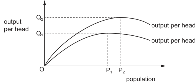
Which change could not satisfactorily explain the shift from year 1 to year 2?
Options
A Population has increased.
B State of technology has improved.
C Stock of capital has increased.
D Volume of productive resources in use has increased.
Reasoning
The diagram shows the output per head curve shifting upwards from year 1 to year 2, with the peak moving from P1 to P2 and from Q1 to Q2. This represents an increase in output per head at any given population size.
An increase in population (option A) would be shown as a movement along the existing curve to the right, resulting in a lower output per head if the new population exceeds the optimum. It would not shift the entire curve upward.
By contrast, an improvement in technology (B), an increase in the stock of capital (C), and an increase in the volume of productive resources in use (D) would all raise productivity and output per head, shifting the curve outward/upward to a new position such as that shown for year 2.
Therefore, the change that could not satisfactorily explain the shift is A.
Answer
A
A
Background Concept
The optimum level of population is the size of population at which real output per head is maximised. The relationship is typically illustrated by an inverted U-shaped curve: as population increases from a low base, output per head rises due to the benefits of the division of labour and the more efficient use of fixed resources; beyond a certain point, however, diminishing returns set in and output per head falls. The peak of the curve represents the optimum population.
A shift of the entire curve outward (upward) indicates that output per head has increased at every level of population. This is caused by factors that raise productivity, such as technological progress, increases in the capital stock, improvements in human capital, or an increase in the availability of other productive resources. By contrast, a change in the size of the population itself is represented by a movement along the existing curve, because population is the variable plotted on the horizontal axis.
Understanding the Question
The diagram displays two curves for two different time periods. The year 2 curve lies entirely above the year 1 curve, and its peak is further to the right (P2 > P1) and higher (Q2 > Q1). This means that in year 2, the economy can sustain a larger population while achieving a higher maximum output per head. The question asks which of the four listed changes could NOT satisfactorily explain this upward shift of the curve.
Approach
To answer this, evaluate each option against the distinction between a shift factor and a movement along the curve:
- If the change affects productivity or the production capacity per person, it shifts the curve.
- If the change is simply a change in the number of people (the x-axis variable), it is a movement along the curve.
Population is the variable on the horizontal axis, so a change in population is a movement along the curve, not a shift. The other three options are all supply-side improvements that would shift the curve upward.
Step-by-Step Reasoning
-
Identify the nature of the change in the diagram. The diagram shows two distinct curves. Year 2 is not a point on the year 1 curve; it is a new curve entirely. This confirms we are looking for a shift factor, not a movement along the original curve.
-
Analyse Option A: Population has increased. If the population grows, the economy moves to a point further right along the horizontal axis. On the year 1 curve, moving right of P1 would actually reduce output per head because the curve slopes downward after the optimum. A population increase does not shift the curve; it moves the economy along it. Therefore, population increase cannot explain why the entire curve has shifted up to the year 2 position.
-
Analyse Option B: State of technology has improved. Better technology raises the productivity of labour and other resources. At any given population size, output per head will be higher. This shifts the entire curve upward and may also move the optimum population to the right. This satisfactorily explains the shift.
-
Analyse Option C: Stock of capital has increased. More capital per worker (e.g., machinery, infrastructure) increases labour productivity. This raises output per head at any given population level, shifting the curve upward. This satisfactorily explains the shift.
-
Analyse Option D: Volume of productive resources in use has increased. Assuming this refers to an increase in non-labour resources or more intensive utilisation, total output rises. With population unchanged, output per head rises, shifting the curve upward. This satisfactorily explains the shift.
-
Conclusion. Only Option A fails to explain the shift because it describes a movement along the curve rather than a shift of the curve itself.
Key Takeaways
- In the optimum population model, population is the independent variable on the horizontal axis; output per head is the dependent variable on the vertical axis.
- A shift of the curve is caused by changes in technology, capital, or other productivity-enhancing factors.
- A movement along the curve is caused by a change in the size of the population.
- When a question asks you to explain a shift of the curve, do not select an option that merely changes the x-axis variable.
Common Mistakes
- Confusing movements with shifts: Students often select population growth as a cause of the shift, forgetting that population is the variable being changed along the x-axis.
- Misreading the diagram: Failing to notice that the year 2 curve is entirely separate from and above the year 1 curve, and instead interpreting the change as a movement along a single curve.
- Overlooking the definition: Forgetting that the curve specifically plots output per head, so any factor raising total output relative to population will shift it.
Things to Be Careful About
- The question specifically asks what could not explain the shift. Be precise about the terminology: a shift versus a movement.
- Ensure you understand that the optimum population (P1 to P2) has increased, which is consistent with productivity improvements, not merely population growth.
- In multiple-choice questions, eliminate the three options that are valid explanations; the remaining option is the correct answer.
A government wants to reduce the current account deficit on the balance of payments.
What is an example of an expenditure-reducing policy?
Options
A a devaluation of the currency
B a subsidy on domestic production
C a tariff on imports
D an increase in income taxes
Answer
Expenditure-reducing policies aim to lower aggregate demand, thereby reducing demand for imports and improving the current account. Of the options, only an increase in income taxes reduces disposable income and consumption, lowering total expenditure and imports. A devaluation (A), a subsidy on domestic production (B), and a tariff (C) are all expenditure-switching policies — they redirect demand from foreign to domestic goods without necessarily cutting overall spending. Therefore the correct answer is D.
D
Background Concept
When a country runs a current account deficit, it means its expenditure on imports of goods and services exceeds its export earnings. Policies to correct the deficit fall into two categories:
- Expenditure-reducing policies – contractionary fiscal or monetary policy that reduces aggregate demand. Lower total spending reduces imports (since imports are a function of income) and may also free up domestic output for export. Examples: higher income taxes, lower government spending, higher interest rates.
- Expenditure-switching policies – measures that divert existing spending away from foreign goods towards domestic goods. These do not necessarily change the total level of spending. Examples: devaluation of the currency (makes exports cheaper, imports dearer), tariffs (make imports more expensive), subsidies on domestic production (lower the relative price of home-produced goods).
Understanding the Question
The question presents a government objective (reduce current account deficit) and asks for an example of an expenditure-reducing policy from four options. It tests the candidate’s ability to distinguish which policy works by cutting total spending rather than by redirecting it.
- A – Devaluation: switches spending to domestic goods; total expenditure unchanged.
- B – Subsidy on domestic production: domestic goods become cheaper relative to imports; total spending unchanged (or may even increase if goods are cheaper).
- C – Tariff on imports: raises import price, switches spending to domestic substitutes; total expenditure unchanged (or may fall if tariff revenue reduces disposable income, but the primary effect is switching).
- D – Increase in income taxes: reduces disposable income, lowering consumption and thus aggregate demand; this reduces import demand directly. This is expenditure-reducing.
Approach
- Recall the definitions of expenditure-reducing and expenditure-switching policies.
- Examine each option in order and classify it based on its primary effect on aggregate demand.
- Identify the option that fits the definition of expenditure-reducing.
Step-by-Step Reasoning
Step 1: Define the two types.
- Expenditure-reducing: contractionary demand-side policies that cut total spending (C+I+G) and therefore imports.
- Expenditure-switching: policies that change relative prices to favour domestic goods, leaving total spending unchanged.
Step 2: Evaluate each option.
- Option A – Devaluation lowers the exchange rate. This makes exports cheaper in foreign currency and imports dearer in domestic currency. Consumers switch from imports to domestic substitutes, but if total spending in domestic currency terms stays the same, the effect is purely switching. (It may also have an expenditure-reducing effect if the Marshall-Lerner condition is not met, but the primary textbook classification is switching.)
- Option B – A subsidy on domestic production lowers production costs. Domestic goods become relatively cheaper than imports, encouraging switching. Total spending may even rise if the subsidy is funded by borrowing, but the intended effect is switching.
- Option C – A tariff raises the price of imports. Consumers switch to domestic goods. Again, switching effect dominates.
- Option D – An increase in income taxes reduces households’ disposable income. This lowers consumption spending and thus aggregate demand. With lower total spending, demand for all goods (including imports) falls. This directly reduces the import bill, improving the current account. No switching is involved; the mechanism is a reduction in the level of expenditure.
Step 3: Conclude – Only D fits the definition of expenditure-reducing policy.
Key Takeaways
- Expenditure-reducing policies work by cutting total spending; expenditure-switching policies work by changing the composition of spending.
- Both can improve the current account, but the distinction is important for understanding macroeconomic policy choice.
- Common expenditure-reducing policies: higher taxes, lower government spending, higher interest rates (contractionary fiscal/monetary policy).
- Common expenditure-switching policies: exchange rate changes, tariffs, subsidies, import quotas.
Common Mistakes
- Mistaking a tariff (C) for expenditure-reducing because it directly reduces import quantities – students forget that tariffs work by switching expenditure, not reducing total spending.
- Thinking devaluation (A) is expenditure-reducing – while devaluation may reduce aggregate demand if it raises import costs for firms, the textbook definition classifies it as switching.
- Overlooking the core mechanism of income taxes – they reduce disposable income and thus total spending, which is clearly expenditure-reducing.
Things to Be Careful About
- Always classify policies by their primary intended mechanism.
- In some real-world contexts, a policy may have both reducing and switching effects (e.g. a tariff could also reduce expenditure if its revenue is not recycled), but in standard A-level analysis the textbook distinction is clear.
- The question asks for an “example”; respond with the specific policy option, not a general description.
During a year, a country’s national income in money terms increased by 5%, prices increased by 4% and the total population increased by 2%.
What was the approximate change in real income per head?
Options
A a decrease of 1%
B a decrease of 2%
C an increase of 1%
D an increase of 2%
Working
Real national income growth ≈ nominal growth – inflation = 5% – 4% = +1%.
Real income per head growth ≈ real income growth – population growth = 1% – 2% = –1%.
Answer
A
A
Background Concept
National income can be measured in nominal (money) terms or real terms. Real national income adjusts for changes in the price level, so it reflects changes in the volume of goods and services produced. Real income per head (per capita) divides real national income by the total population, providing a measure of average living standards. Small percentage changes in these variables can be approximated using the formula: percentage change in real variable ≈ percentage change in nominal variable – percentage change in price level. Similarly, percentage change in per capita variable ≈ percentage change in total variable – percentage change in population.
Understanding the Question
This question provides three percentage changes: nominal national income increased by 5%, prices increased by 4%, and population increased by 2%. We are asked to find the approximate change in real income per head. The question tests the ability to apply the above approximations correctly.
Approach
First, compute the percentage change in real national income by subtracting the inflation rate from the nominal growth rate. Then, compute the percentage change in real income per head by subtracting the population growth rate from the real income growth rate. The result is a decrease of approximately 1%.
Step-by-Step Reasoning
- Real national income growth ≈ nominal national income growth – inflation = 5% – 4% = +1%. This means the total real output of the economy increased by about 1%.
- Real income per head growth ≈ real national income growth – population growth = 1% – 2% = –1%. This means that, on average, each person’s real income fell by about 1%.
- Therefore, the approximate change is a decrease of 1%, which corresponds to option A.
To check: exact calculation using multiplicative factors: (1.05/1.04)/1.02 – 1 = (1.009615)/1.02 – 1 = 0.9898 – 1 = –0.0102, i.e., –1.02%, so the approximation is very close.
Key Takeaways
- Real income growth is approximately nominal growth minus inflation.
- Per capita growth is approximately total growth minus population growth.
- These approximations work well for small percentage changes.
- Understanding the distinction between nominal and real values is crucial in macroeconomics.
Common Mistakes
- Forgetting to adjust for inflation first and then population, or applying the adjustments in the wrong order.
- Adding the population growth instead of subtracting it, leading to an incorrect increase.
- Confusing real income per head with total real income, and thus not accounting for population growth.
- Using the exact calculation but then misinterpreting the sign.
Things to Be Careful About
- The approximation is only valid for small percentage changes. For large changes, the multiplicative formula should be used exactly.
- Always consider the sign: an increase in population reduces per capita income if total income is unchanged.
- Ensure that the units are consistent (all percentage changes).
- In this question, the wording “approximate change” signals that the approximation method is acceptable.
What is most likely to result from foreign direct investment in a developing economy?
Options
A an improvement in the developing economy’s trade balance
B an increase in the developing economy’s net investment income
C a reduction in the developing economy’s government tax revenue
D a reduction in wage levels in the developing economy
Reasoning
Foreign direct investment (FDI) involves a firm from one country establishing a physical presence in another, such as building a factory or acquiring a local company. This typically leads to the construction of new productive capacity and the import of capital equipment. Once operational, the new subsidiary often exports a significant share of its output, either back to the parent company's home market or to third countries. The resulting increase in exports directly improves the developing economy's trade balance (exports minus imports of goods).
Option B is incorrect because the profits earned by the foreign-owned subsidiary are repatriated as investment income outflows, which worsen the net investment income component of the current account. Option C is incorrect because the new economic activity generates additional corporate tax and employment taxes, increasing government revenue. Option D is incorrect because FDI typically raises the demand for labour in the host economy, putting upward pressure on wages, not reducing them.
Answer
A
A
Background Concept
Foreign Direct Investment (FDI) is a cross-border investment in which a resident entity in one economy acquires a lasting interest in an enterprise in another economy. 'Lasting interest' implies the existence of a long-term relationship and a significant degree of influence by the investor on the management of the enterprise. This is distinct from portfolio investment, which is the purchase of foreign stocks or bonds for purely financial return without control. The key consequences of FDI for a host developing economy typically include: capital inflow for construction, technology and skills transfer, increased competition, access to export markets, and the creation of jobs. However, it also involves profit repatriation, which is a debit on the current account's primary income (investment income) balance.
Understanding the Question
This is a multiple-choice question asking for the single most likely outcome of FDI in a developing economy. The question tests the candidate's understanding of the typical balance of payments effects of FDI. The four options present plausible but mostly incorrect consequences. The correct answer is the one that is most consistently observed in the data and economic theory: an improvement in the trade balance. The question requires distinguishing between the trade balance effect (goods and services) and the primary income effect (profits and dividends).
Approach
- Recall the definition and typical sequence of events following an FDI inflow.
- Consider the immediate effect on the capital account (inflow of funds for the investment) and the subsequent effect on the current account.
- Evaluate each option against this sequence:
- Option A (Trade balance): FDI creates new productive capacity. The new subsidiary often imports capital goods initially, but then exports its output. The net effect on the trade balance is typically positive in the medium to long term.
- Option B (Net investment income): FDI generates profits for the foreign owner. These profits are repatriated, which is a debit on the investment income account. This worsens net investment income.
- Option C (Government tax revenue): FDI increases economic activity, which broadens the tax base (corporate tax, income tax, VAT). This increases government revenue.
- Option D (Wage levels): FDI increases the demand for labour, especially in the sector receiving the investment. This tends to raise, not reduce, wage levels.
- Select the option that is most consistent with the standard analysis.
Step-by-Step Reasoning
- Define FDI: A firm from a developed country (e.g., a car manufacturer) decides to build a factory in a developing economy (e.g., Thailand). This involves a capital inflow to purchase land, build the factory, and buy machinery.
- Trace the trade balance effect:
- Initial phase: The factory imports machinery and specialised inputs. This increases imports, worsening the trade balance temporarily.
- Operational phase: The factory produces cars. A large proportion of these cars are exported to regional or global markets. The value of these exports is a credit on the trade balance. The net effect over the life of the investment is almost always a significant improvement in the trade balance, as the exports generated far exceed the initial import of capital goods.
- Trace the investment income effect: The factory generates profits. These profits are owned by the foreign parent company. When the profits are sent back to the parent company's home country, they are recorded as a debit on the 'primary income' (or investment income) account of the current account. This worsens the net investment income balance. Therefore, option B is incorrect.
- Trace the government revenue effect: The factory pays corporate income tax on its profits. Its workers pay income tax. The purchase of local inputs generates VAT. All of these increase government tax revenue. Therefore, option C is incorrect.
- Trace the wage effect: The factory hires local workers. This increases the demand for labour in the local economy. All else equal, this increased demand pushes wages up, not down. FDI is often associated with higher wages than local firms pay. Therefore, option D is incorrect.
- Conclusion: The most likely and most significant macroeconomic result of FDI is an improvement in the host country's trade balance, as the new productive capacity is export-oriented. While there is a negative effect on investment income, the trade balance effect is typically larger and more direct.
Key Takeaways
- FDI is a capital inflow that creates productive capacity.
- The primary current account benefit of FDI is an improved trade balance (exports of goods).
- The primary current account cost of FDI is profit repatriation, which worsens the investment income balance.
- FDI typically increases government revenue and raises wage levels in the host economy.
- It is crucial to distinguish between the trade balance (goods and services) and the primary income balance (profits, dividends, interest) when analysing the balance of payments effects of FDI.
Common Mistakes
- Confusing FDI with portfolio investment: A student might think FDI is just a financial flow and focus only on the capital account, ignoring the real economic effects on trade.
- Focusing only on profit repatriation: A student might correctly identify that profits are repatriated (a debit on investment income) and incorrectly conclude that this makes the current account worse overall, forgetting that the trade balance improvement is usually larger.
- Assuming FDI always exploits labour: A common misconception is that FDI lowers wages. While there can be cases of exploitation in some sectors, the standard economic effect is an increase in labour demand and therefore higher wages.
- Ignoring the time horizon: The question asks for the 'most likely' result. The trade balance improvement is a medium-to-long-term result. A student might focus on the short-term import of capital goods and incorrectly choose a different option.
Things to Be Careful About
- Read the question carefully: It asks for the 'most likely' result. All options have some theoretical basis, but only one is the standard, well-established consequence.
- Distinguish between the trade balance and the current account: The trade balance is a component of the current account. The question specifically asks about the trade balance, not the overall current account.
- Understand the direction of flows: FDI is a capital inflow (credit on the financial account). Profit repatriation is a current account debit. Exports generated by the FDI are a current account credit. Keeping these flows straight is essential.
The diagram shows an economy’s Lorenz curve (VW).
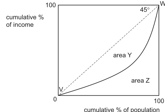
How is the Gini coefficient for the economy calculated?
Options
A Y / (Y + Z)
B Y / Z
C Z / Y
D Z / (Y + Z)
Reasoning
The Gini coefficient measures income inequality, calculated as the ratio of the area between the line of perfect equality (the 45-degree line) and the Lorenz curve (area Y) to the total area under the line of perfect equality (area Y + area Z). This matches option A.
Answer
A
A
Background Concept
The Lorenz curve is a graphical tool used to represent income or wealth distribution within an economy. The horizontal axis plots the cumulative percentage of the population (ordered from lowest to highest income/wealth), and the vertical axis plots the cumulative percentage of total income/wealth held by that population group. The 45-degree line of perfect equality runs from the origin (0,0) to the top-right corner (100,100), representing a scenario where every percentage of the population earns exactly the same percentage of total income (for example, the bottom 20% of the population earns 20% of total income). The further the Lorenz curve lies below this line of equality, the greater the level of income inequality in the economy.
The Gini coefficient is a numerical summary measure of income inequality, ranging from 0 (perfect equality, where the Lorenz curve coincides exactly with the line of equality) to 1 (perfect inequality, where all income is held by a single individual, so the Lorenz curve runs along the bottom and right edges of the graph). It is calculated as the ratio of the area between the line of equality and the Lorenz curve (area Y in the diagram) to the total area under the line of equality (the sum of area Y and area Z, which forms a right triangle with base and height both equal to 100 on the axes).
Understanding the Question
This 1-mark multiple-choice question asks you to identify the correct formula for calculating the Gini coefficient using the labelled areas on the provided Lorenz curve diagram. The diagram labels the area between the 45-degree line of equality and the Lorenz curve as Y, and the area below the Lorenz curve (between the curve and the axes) as Z. You need to match these labelled areas to the standard Gini coefficient formula to select the correct option.
Approach
To answer this question, you only need to recall the standard definition and formula for the Gini coefficient, then match the labelled areas in the diagram to the components of the formula. No calculation or analysis is required, as this is a recall question testing your knowledge of the Lorenz curve and Gini coefficient.
Step-by-Step Reasoning
- First, recall the formula for the Gini coefficient: G = A / (A + B), where:
- A = the area between the line of perfect equality and the Lorenz curve (this measures the deviation from perfect equality)
- B = the area under the Lorenz curve (this measures the actual cumulative income share held by the cumulative population share)
- The denominator (A + B) is the total area under the line of perfect equality, which is the area of the right triangle formed by the 45-degree line and the two axes.
- Match these components to the labelled areas in the diagram:
- Area Y is the area between the 45-degree line of equality and the Lorenz curve, so this corresponds to A in the formula.
- Area Z is the area under the Lorenz curve, so this corresponds to B in the formula.
- Substitute the labelled areas into the formula: G = Y / (Y + Z).
- Compare this to the options: this matches option A. The other options are incorrect: option B (Y/Z) is the ratio of the inequality area to the equality area, which is not the Gini; option C (Z/Y) is the inverse of that; option D (Z/(Y+Z)) is the share of the total area that lies under the Lorenz curve, which equals 1 minus the Gini coefficient.
Key Takeaways
- The Lorenz curve visually represents income inequality, with deviation from the 45-degree line of equality indicating higher inequality.
- The Gini coefficient is a standardised measure of inequality calculated as the ratio of the area between the equality line and the Lorenz curve to the total area under the equality line.
- A Gini coefficient of 0 means perfect equality, while a value closer to 1 means higher inequality.
Common Mistakes
- Mixing up the areas: confusing area Y (between the lines) with area Z (under the Lorenz curve), leading to selecting options C or D.
- Forgetting that the denominator is the total area under the line of equality (Y + Z), not just area Z or area Y, leading to selecting options B or C.
- Misremembering the formula as the ratio of the area under the Lorenz curve to the total area, which would give option D, the inverse of the correct Gini coefficient.
Things to Be Careful About
- Always check which area is which on the diagram: the area between the two lines is the numerator, the total area under the equality line is the denominator.
- Remember that the Gini coefficient ranges from 0 to 1, so the formula must produce a value in this range. Option D would give a value between 0 and 1 as well, but it is the complement of the Gini, not the Gini itself, so it is incorrect.
The table gives the percentage of employment in the primary, secondary and tertiary sectors in four countries.
Which country is most likely to be a high-income country?
Options
| primary sector % | secondary sector % | tertiary sector % | |
|---|---|---|---|
| A | 15 | 40 | 45 |
| B | 30 | 40 | 30 |
| C | 35 | 45 | 20 |
| D | 45 | 35 | 20 |
Reasoning
High-income countries typically have a large tertiary (services) sector and a small primary sector. Among the options, Country A has the highest tertiary sector share (45%) and the lowest primary sector share (15%), indicating a post-industrial economy. Country B has a balanced structure, Country C has a large secondary sector, and Country D has a large primary sector, all more characteristic of lower-income economies.
Answer
A
A
Background Concept
As economies develop, they undergo structural change: employment shifts from the primary sector (agriculture, mining, fishing) to the secondary sector (manufacturing, construction) and then to the tertiary sector (services). High-income countries are typically post-industrial, with a dominant tertiary sector (often over 70% of employment) and a very small primary sector. Middle-income countries often have a large secondary sector, while low-income countries have a large primary sector.
Understanding the Question
The question provides employment percentages for four countries and asks which is most likely to be a high-income country. We need to apply the typical pattern of structural change to identify the country whose employment structure most closely resembles that of a high-income economy.
Approach
Compare the shares across the three sectors for each country. High-income countries have low primary and high tertiary. Country A has 15% primary and 45% tertiary; Country B has 30% primary and 30% tertiary; Country C has 35% primary and 20% tertiary; Country D has 45% primary and 20% tertiary. Country A is the best match.
Step-by-Step Reasoning
- Country A: Primary 15%, Secondary 40%, Tertiary 45%. The primary sector is relatively small, and the tertiary sector is the largest. This structure is consistent with a high-income economy that has moved beyond manufacturing into services.
- Country B: Primary 30%, Secondary 40%, Tertiary 30%. The primary sector is still significant, and the tertiary sector is not dominant. This suggests a middle-income economy still industrialising.
- Country C: Primary 35%, Secondary 45%, Tertiary 20%. The secondary sector is the largest, and the tertiary sector is small. This is typical of an industrialising economy, not a high-income one.
- Country D: Primary 45%, Secondary 35%, Tertiary 20%. The primary sector dominates, indicating a low-income, agriculture-based economy.
Therefore, Country A is the most likely to be a high-income country.
Key Takeaways
- Employment structure is a key indicator of a country's level of development.
- High-income economies are characterised by a large tertiary sector and a small primary sector.
- The shift from primary to secondary to tertiary is known as the Clark-Fisher hypothesis or structural change.
Common Mistakes
- Assuming a large secondary sector indicates high income (many high-income countries have deindustrialised, so a large secondary sector is more typical of middle-income countries).
- Not comparing all three sectors together; focusing only on one sector can lead to incorrect conclusions.
- Misreading the table or not noticing that the percentages sum to 100%.
Things to Be Careful About
- Ensure you interpret the data correctly: high-income countries have low primary and high tertiary.
- The percentages in each row sum to 100%, so the relative sizes are directly comparable.
- This is a simple application of a well-known pattern; no calculation is needed.
Your score so far
Answer a question to start scoring
Your marks add up here as you work through the paper.