Economics 9708/32 — October/November 2024
Cambridge A-Level · A Level Multiple Choice · answer key with instant marking and worked solutions
Topics Externalities, Social Costs and Benefits · Macroeconomic Objectives and Policy Conflicts · Balance of Payments and Policies to Correct Disequilibrium · Costs of Production · Wage Determination and Labour Market Intervention · Demand for and Supply of Labour · +17 more
Tap an option under each question to check it — your score builds as you go.
If consumers aim to maximise their utility, how will they arrange their spending?
Options
A to obtain the same total utility from each commodity
B to obtain the same total utility per $ spent on each commodity
C to obtain the same utility from the last unit of each commodity
D to obtain the same utility from the last $ spent on each commodity
Answer
Consumers maximise utility by allocating their budget so that the marginal utility per dollar (or per unit of currency) spent is equal across all goods. This is the equi-marginal principle. Option D correctly states this condition: 'to obtain the same utility from the last $ spent on each commodity'.
D
Background Concept
This question tests the equi-marginal principle, which is the core rule for how a rational consumer maximises total utility given a limited budget. The principle states that a consumer should allocate their spending across different goods so that the marginal utility per unit of currency (MU per $) is equal for every good consumed. If MU per $ is higher for good A than for good B, the consumer can increase total utility by spending one more dollar on A and one less on B. This reallocation continues until the MU per $ is equalised across all goods. At that point, no further reallocation can increase total utility, so the consumer is maximising utility.
Understanding the Question
The question asks: 'If consumers aim to maximise their utility, how will they arrange their spending?' It provides four options, each describing a different possible rule. The key is to identify which rule correctly describes the condition for utility maximisation. The options confuse total utility with marginal utility, and the total spent with the last unit spent.
Approach
Recall the equi-marginal principle. The condition for utility maximisation is that the marginal utility per dollar spent is equal across all goods. This is expressed as MUa/Pa = MUb/Pb = ... = MUn/Pn. The correct option must refer to 'the last $ spent' (marginal) and 'the same utility' (marginal utility) per dollar. Eliminate options that refer to total utility or to the same utility from the last unit (without considering price).
Step-by-Step Reasoning
- Option A: 'to obtain the same total utility from each commodity'. This is incorrect. A consumer does not aim for equal total utility from each good; they aim to maximise the sum of total utility across all goods, which typically involves different total utilities from different goods.
- Option B: 'to obtain the same total utility per $ spent on each commodity'. This is also incorrect. It refers to total utility per dollar, which is not the maximisation condition. The condition involves marginal utility, not total utility.
- Option C: 'to obtain the same utility from the last unit of each commodity'. This is close but misses the crucial element of price. It says 'the same utility from the last unit', which is marginal utility (MU). However, it ignores the cost of that unit. If good A has a MU of 10 and costs $1, while good B has a MU of 10 but costs $2, the consumer gets more 'bang for the buck' from good A. The condition must account for price.
- Option D: 'to obtain the same utility from the last $ spent on each commodity'. This is correct. 'The last $ spent' means the marginal dollar, and 'the same utility' refers to the marginal utility obtained from that last dollar. This is exactly the equi-marginal principle: MUa/Pa = MUb/Pb = ... = MUn/Pn. The consumer adjusts spending until the extra utility gained from the last dollar spent on each good is equal.
Key Takeaways
- Utility maximisation is about equalising marginal utility per dollar, not total utility or marginal utility alone.
- The equi-marginal principle is the fundamental rule for rational consumer choice under a budget constraint.
- Always distinguish between total utility (satisfaction from all units) and marginal utility (satisfaction from the last unit).
Common Mistakes
- Confusing total and marginal utility: Many students pick option A or B because they think about 'total' satisfaction, but the decision at the margin is what matters for optimisation.
- Forgetting the price: Option C is a common trap because it correctly identifies marginal utility but omits the price of the good. The condition must be MU per unit of currency, not just MU.
- Misreading the wording: 'The last $ spent' is a clear reference to the marginal dollar, but some students may misinterpret it as 'the last unit'.
Things to Be Careful About
- Read each option carefully. The difference between 'last unit' and 'last $' is the key distinction between C and D.
- Remember that the equi-marginal principle is the foundation for deriving the law of demand: when the price of a good falls, its MU per $ rises, leading the consumer to buy more of it until MU per $ is again equalised.
Which feature of indifference curve theory is most likely to apply in reality?
Options
A The consumer can express preferences between all possible combinations of goods.
B The consumer has a limited income to spend.
C The consumer will always behave rationally.
D The consumer will always get positive utility from having more of the goods.
Answer
Indifference curve theory assumes the consumer has a limited income, which is realistic because consumers face budget constraints. The other assumptions are often unrealistic: complete preferences (A) are rarely held for all possible combinations, rational behaviour (C) is frequently violated by behavioural biases, and positive utility from more goods (D) ignores satiation and the possibility of 'bads'. Therefore, the feature most likely to apply in reality is that the consumer has a limited income.
Answer
B
B
Background Concept
Indifference curve theory is a model of consumer choice that uses indifference curves (showing combinations of goods giving equal satisfaction) and a budget line (showing affordable combinations given income and prices). The model relies on several key assumptions: completeness (the consumer can rank all bundles), rationality (consistent preferences), non-satiation (more is always better), and a limited income (budget constraint). These assumptions simplify analysis but may not hold in reality.
Understanding the Question
The question asks which feature of indifference curve theory is most likely to apply in reality. It tests your understanding of which assumptions are realistic descriptions of actual consumer behaviour and which are simplifying abstractions. The correct answer is B: the consumer has a limited income to spend.
Approach
Evaluate each option against real-world consumer behaviour:
- A: Can consumers truly express preferences between every possible combination? Usually not – preferences are often incomplete or vague.
- B: Do consumers have a limited income? Yes, almost always – this is a fundamental constraint.
- C: Do consumers always behave rationally? No – behavioural economics shows systematic deviations.
- D: Do consumers always get positive utility from more of a good? No – satiation, diminishing marginal utility, and 'bads' mean more is not always better.
Step-by-Step Reasoning
- Option A: Indifference curve theory assumes completeness – the consumer can compare any two bundles and state a preference or indifference. In reality, consumers often face uncertainty or lack information, making it impossible to rank all bundles. This assumption is unrealistic.
- Option B: The budget line represents the consumer's limited income. In reality, almost all consumers have a finite income and must make choices within that constraint. This is a realistic and universal feature.
- Option C: Rationality implies transitive and consistent preferences. Real consumers are influenced by framing, emotions, and cognitive biases, violating rationality. This assumption is unrealistic.
- Option D: Non-satiation assumes more of a good always increases utility. However, after a point, additional consumption may yield zero or negative utility (e.g., overeating). This assumption is unrealistic.
Thus, only option B is a feature that holds in reality.
Key Takeaways
- Indifference curve theory is a useful model but relies on simplifying assumptions.
- The budget constraint (limited income) is the most realistic assumption.
- Understanding which assumptions are realistic helps evaluate the model's applicability.
Common Mistakes
- Choosing A or D because they seem intuitive, without recognising that preferences are often incomplete and that more is not always better.
- Assuming that because the model is taught, all its assumptions must be realistic.
- Overlooking that rationality is a strong assumption often contradicted by real behaviour.
Things to Be Careful About
- The question asks for the feature 'most likely to apply in reality' – it is a comparative judgement, not an absolute one.
- Do not confuse the assumptions of indifference curve theory with those of other models (e.g., utility theory).
- Remember that 'limited income' is a constraint, not a behavioural assumption.
Diagrams 1 and 2 show different long-run average cost curves (LRAC).
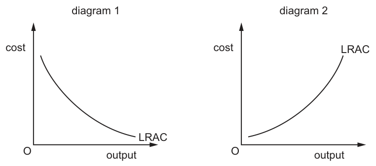
Which situations do the two diagrams show?
Options
| diagram 1 | diagram 2 | |
|---|---|---|
| A | falling returns to scale | average cost is greater than marginal cost |
| B | falling returns to scale | rising returns to scale |
| C | unit cost falls as output increases | falling average fixed costs |
| D | unit cost falls as output increases | unit cost rises as output increases |
Reasoning
A downward-sloping long-run average cost (LRAC) curve, as shown in diagram 1, means that as output increases, the unit (average) cost of production falls. An upward-sloping LRAC curve, as shown in diagram 2, means that as output increases, unit cost rises.
Eliminating other options:
- Option A is incorrect because the LRAC curve alone does not show the relationship between average cost and marginal cost.
- Option B is incorrect because an upward-sloping LRAC reflects falling (not rising) returns to scale.
- Option C is incorrect because average fixed cost is a short-run concept; in the long run all costs are variable, so average fixed cost does not exist.
Only option D correctly describes both diagrams.
Answer
D
D
Background Concept
The long-run average cost (LRAC) curve shows the minimum average (unit) cost of producing any given level of output when all factors of production are variable, and the firm can adjust all its inputs to the optimal size for that output level. The shape of the LRAC curve is determined by returns to scale:
- A downward-sloping LRAC means that as output increases, unit cost falls. This occurs when the firm experiences increasing returns to scale (economies of scale): output rises proportionally more than input costs, so average cost per unit falls.
- A flat LRAC means unit cost stays constant as output increases, corresponding to constant returns to scale.
- An upward-sloping LRAC means that as output increases, unit cost rises. This occurs when the firm experiences decreasing returns to scale (diseconomies of scale): input costs rise proportionally more than output, so average cost per unit rises.
It is important to distinguish long-run and short-run cost curves: in the short run, some factors are fixed, so fixed costs exist, and average fixed cost (AFC) falls as output rises. In the long run, there are no fixed costs, so AFC is not a relevant concept for LRAC analysis. Additionally, the relationship between average cost (AC) and marginal cost (MC) cannot be determined from the LRAC curve alone — the MC curve must be plotted alongside the AC curve to see whether MC is above or below AC at a given output.
Understanding the Question
The question presents two LRAC diagrams: Diagram 1 is downward-sloping, and Diagram 2 is upward-sloping. The task is to select the option that correctly describes what each diagram represents. This is a 1-mark multiple-choice question testing basic recall of LRAC curve properties and related cost concepts.
Approach
First, recall the meaning of different LRAC slopes and the definitions of key terms (returns to scale, average fixed cost, relationship between AC and MC). Then, evaluate each option against this theory to eliminate incorrect choices, and select the option where both descriptions match the diagrams and economic theory.
Step-by-Step Reasoning
We evaluate each option in turn:
- Option A: Claims Diagram 2 shows average cost is greater than marginal cost. The LRAC curve only plots average cost against output; it does not include the marginal cost curve, so there is no information to judge whether AC is above or below MC. This description is unsupported, so A is incorrect.
- Option B: Claims Diagram 2 shows rising returns to scale. Upward-sloping LRAC is caused by decreasing (falling) returns to scale (diseconomies of scale), where unit costs rise as output expands. Rising returns to scale would cause LRAC to fall, not rise. So B is incorrect.
- Option C: Claims Diagram 2 shows falling average fixed costs. Average fixed cost is a short-run concept: in the short run, fixed costs are spread over more units as output rises, so AFC falls. In the long run, all costs are variable, so there are no fixed costs and no average fixed cost. This description is impossible for a long-run curve, so C is incorrect.
- Option D: Claims Diagram 1 shows unit cost falls as output increases, and Diagram 2 shows unit cost rises as output increases. A downward-sloping LRAC (Diagram 1) directly means that as output (x-axis) increases, cost per unit (y-axis) falls. An upward-sloping LRAC (Diagram 2) directly means that as output increases, cost per unit rises. Both descriptions are fully consistent with the diagrams and economic theory, so D is the correct answer.
Key Takeaways
- The slope of the LRAC curve directly indicates how unit cost changes with output: downward = falling unit cost, upward = rising unit cost.
- Returns to scale and LRAC slope are inversely related for "rising/falling" labels: increasing returns to scale = falling LRAC, decreasing returns to scale = rising LRAC.
- Average fixed cost only exists in the short run; it is not a relevant concept for long-run cost curves.
- The relationship between average and marginal cost cannot be inferred from the LRAC curve alone.
Common Mistakes
- Confusing the direction of returns to scale: many students incorrectly associate upward-sloping LRAC with rising returns to scale, when it is actually associated with falling returns to scale.
- Forgetting the short-run/long-run distinction: applying short-run concepts like average fixed cost to long-run curves, which have no fixed costs.
- Assuming the LRAC curve shows the MC-AC relationship: the LRAC is an envelope of short-run AC curves, but it does not plot MC, so no conclusion about MC can be drawn from it alone.
Things to Be Careful About
- Always check whether a cost concept is short-run or long-run before applying it: fixed costs and AFC are short-run only.
- When matching curve shapes to economic concepts, be precise about direction: "rising returns to scale" leads to falling unit costs, not rising.
- For multiple-choice questions, eliminate options that rely on information not present in the diagram (like the MC-AC relationship here, which is not shown).
A government makes it compulsory for motorbike riders to wear helmets.
What would represent a positive externality of consumption associated with this decision?
Options
A decreased pressure on the provision of health care
B expenses incurred on surveillance of motorbike riders to ensure compliance
C increased life expectancy of motorbike riders
D increased profits of helmet manufacturers
Working
A positive externality of consumption arises when the consumption of a good or service benefits third parties not directly involved in the transaction. Compulsory helmet use reduces head injuries among riders, which lowers the burden on public healthcare systems. This benefit to society is not reflected in the market price; hence it is an external benefit.
Option B is a cost incurred by the government, not a benefit. Option C is a private benefit to the rider. Option D is a private benefit to producers.
Answer
A
A
Background Concept
A positive externality of consumption occurs when the consumption of a good or service by an individual generates benefits for third parties who are not directly involved in the transaction. The third parties do not pay for these benefits, and the consumer does not take them into account when deciding how much to consume. As a result, the market underallocates resources to the good or service, leading to a welfare loss. Governments often intervene to correct this market failure, for example by making consumption compulsory (as with helmet laws) or by subsidising the good.
Understanding the Question
The government makes it compulsory for motorbike riders to wear helmets. The question asks which of the listed options represents a positive externality of consumption associated with this decision. This means we need to identify an external benefit – a benefit that accrues to third parties, not to the riders themselves or to producers.
Approach
First, define 'positive externality of consumption'. Then evaluate each option in turn to see if it matches the definition: a benefit to society (third parties) arising from the consumption (use) of helmets, which is not captured by the market price.
Step-by-Step Reasoning
-
Option A: decreased pressure on the provision of health care. When riders wear helmets, fewer serious head injuries occur. This reduces the demand for medical treatment, freeing up healthcare resources for others. The benefit of reduced healthcare strain goes to taxpayers and other patients – third parties. This is a typical example of a positive externality of consumption. Correct.
-
Option B: expenses incurred on surveillance of motorbike riders to ensure compliance. This is a cost to the government (and ultimately taxpayers), not a benefit. Externalities are effects on third parties, but this is a deliberate enforcement cost, not an unintended benefit. It is a negative side-effect (a cost) rather than a positive externality. Incorrect.
-
Option C: increased life expectancy of motorbike riders. This is a direct benefit to the riders themselves – the consumers of helmets. It is a private benefit, not an external benefit. While society might value longer lives, the primary beneficiary is the rider, and it is a private benefit reflected in the rider's own welfare. Incorrect.
-
Option D: increased profits of helmet manufacturers. This is a benefit to producers, arising from increased demand for helmets due to the compulsory law. This is a private benefit to firms, not an externality of consumption. Even if it could be considered a positive effect on the supplier side, it is not an externality of consumption because it is captured in market transactions. Incorrect.
Therefore, only option A correctly identifies a positive externality of consumption.
Key Takeaways
- Positive externalities of consumption are third-party benefits that arise from the act of consuming a good or service.
- They must be distinguished from private benefits (which accrue to the consumer) and producer benefits.
- Costs incurred by the government to enforce a policy are not externalities; they are part of the policy's implementation cost.
- The presence of positive externalities provides a rationale for government intervention to increase consumption of merit goods.
Common Mistakes
- Confusing private benefits (e.g., increased life expectancy) with external benefits. The rider's own life expectancy is a private benefit, even though it may also reduce costs for others. The question specifically asks for externality of consumption.
- Thinking that any positive outcome of a policy is an externality. Profits for manufacturers are a market effect, not an externality.
- Interpreting a reduction in cost (e.g., decreased pressure on healthcare) as a negative event, when in fact it is a benefit (fewer resources used).
- Selecting option B because it is associated with the policy but forgetting that externalities are unintended side-effects, not deliberate costs of enforcement.
Things to Be Careful About
- Always identify the parties: who benefits? If the beneficiary is the consumer or producer directly involved in the transaction, it is a private benefit, not an externality.
- The phrase 'consumption' in 'externality of consumption' means the benefit must arise from the act of consuming the product (here, wearing the helmet).
- A positive externality is a benefit to third parties; a reduction in a negative burden (like less strain on healthcare) is qualitatively a benefit and counts as a positive externality.
- Read all options carefully; sometimes distractors are designed to seem plausible but involve costs or private benefits.
The table shows the market shares of firms selling a very similar product in a country between 2018 and 2020.
| firm | 2018 | 2020 |
|---|---|---|
| Norton | 28.4 | 27.4 |
| Souton | 18.9 | 17.6 |
| Eastern | 17.1 | 14.7 |
| Western | 12.5 | 11.4 |
| Scotsdale | 7.2 | 8.5 |
| Welshpool | 5.8 | 8.2 |
| Greenland | 3.9 | 4.8 |
| Franklin | 2.2 | 3.6 |
| Bellweather | 2.1 | 1.9 |
| others | 1.9 | 1.9 |
What can be concluded from the data between the two years?
Options
A Market concentration increased.
B Sales of the top four firms fell.
C Scotsdale and Welshpool’s profits rose.
D The concentration ratio of the four largest firms fell.
Working
Four-firm concentration ratio (CR4) = sum of market shares of the four largest firms.
2018: Norton (28.4) + Souton (18.9) + Eastern (17.1) + Western (12.5) = 76.9%
2020: Norton (27.4) + Souton (17.6) + Eastern (14.7) + Western (11.4) = 71.1%
The CR4 fell from 76.9% to 71.1%, so market concentration decreased.
Answer
D
D
Background Concept
The concentration ratio is a measure of market concentration, indicating the extent to which a market is dominated by a few large firms. The four-firm concentration ratio (CR4) sums the market shares of the four largest firms. A higher CR4 suggests less competition and more market power. Market share is the percentage of total sales in the market held by a firm.
Understanding the Question
We are given a table of market shares for firms in a country between 2018 and 2020. The question asks what can be concluded from the data. The options test understanding of concentration, sales, and profits. Only the concentration ratio can be directly calculated from market shares; sales and profits require additional data not provided.
Approach
- Calculate the CR4 for 2018 and 2020.
- Compare the two values to see if concentration increased or decreased.
- Evaluate each option: A (market concentration increased) is false if CR4 fell; B (sales of top four firms fell) cannot be determined because market shares are percentages, not absolute sales; C (Scotsdale and Welshpool’s profits rose) cannot be determined because profits depend on costs and prices, not just market share; D (the concentration ratio of the four largest firms fell) is directly supported by the calculation.
Step-by-Step Reasoning
- Identify the four largest firms in each year. In both years, the top four by market share are Norton, Souton, Eastern, and Western (the order is the same).
- Calculate CR4 for 2018: 28.4 + 18.9 + 17.1 + 12.5 = 76.9%.
- Calculate CR4 for 2020: 27.4 + 17.6 + 14.7 + 11.4 = 71.1%.
- The CR4 fell by 5.8 percentage points, indicating that market concentration decreased. Therefore, option A is incorrect and option D is correct.
- Option B: Sales of the top four firms fell. Market shares are relative; even if market shares fell, total market sales could have increased, so absolute sales might have risen. Without total sales data, we cannot conclude. Hence B is not supported.
- Option C: Scotsdale and Welshpool’s profits rose. Profits depend on revenue and costs. Their market shares increased (Scotsdale from 7.2% to 8.5%, Welshpool from 5.8% to 8.2%), but this does not guarantee higher profits; costs could have risen or prices fallen. Thus C cannot be concluded.
Key Takeaways
- The concentration ratio is calculated from market shares, not absolute sales.
- Changes in market shares do not directly imply changes in sales or profits.
- To conclude about sales, we need total market sales data; for profits, we need cost and price information.
Common Mistakes
- Assuming that a fall in market share means a fall in sales (ignoring possible market growth).
- Assuming that a rise in market share means a rise in profits (ignoring costs).
- Misidentifying the four largest firms if the ranking changes.
Things to Be Careful About
- Always use the correct firms for the concentration ratio: the four largest by market share in each year.
- Remember that market shares are percentages; they sum to 100% (or close, due to rounding).
- Do not infer beyond the data given; stick to what can be directly calculated or logically deduced.
The diagram shows a profit maximising firm in equilibrium.
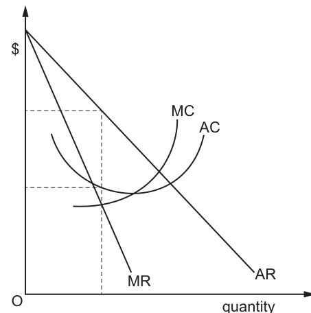
What would happen to the firm’s price, output and profit if there was an increase in its fixed costs?
Options
| price | output | profit | |
|---|---|---|---|
| A | rise | fall | rise |
| B | rise | fall | fall |
| C | unchanged | rise | rise |
| D | unchanged | unchanged | fall |
Reasoning
Fixed costs do not affect marginal cost (MC) because MC is derived from variable costs only. The profit-maximising output is determined where MR = MC. Since MC is unchanged, output remains unchanged. Price is set by the AR curve at this output, so price is also unchanged. Profit equals total revenue minus total cost. With price and output unchanged, total revenue is unchanged, but total cost rises by the increase in fixed costs. Therefore, profit falls.
Answer
D
D
Background Concept
Fixed costs are costs of production that do not vary with the level of output, such as rent, interest on capital, or salaries of permanent staff. Variable costs change directly with output, such as raw materials and hourly wages. Marginal cost (MC) is the additional cost of producing one more unit of output. Because fixed costs do not change when output changes, they do not contribute to marginal cost; MC is derived solely from changes in variable costs.
A profit-maximising firm chooses the output where marginal revenue (MR) equals marginal cost (MC). At this output, the price is determined by the average revenue (AR) curve (which represents the demand curve). Profit is calculated as total revenue (TR) minus total cost (TC), or equivalently as (price minus average cost) multiplied by output.
Understanding the Question
The diagram shows a firm with market power (downward-sloping AR and MR curves) in short-run equilibrium. The firm is producing where MC intersects MR, and charging the price given by the AR curve at that quantity. The question asks what happens to the firm's price, output, and profit if its fixed costs increase.
This is a test of understanding the distinction between fixed and variable costs, and how costs affect firm decisions. The command word is implicit (what would happen), requiring analysis of the causal chain from the cost change to the three outcome variables.
Approach
The key insight is that fixed costs are irrelevant for marginal decisions. Because they do not change with output, they do not affect the MC curve. Therefore:
- The MR = MC condition still gives the same output.
- The AR curve is unchanged, so price is unchanged.
- Profit falls because total cost has increased while total revenue is unchanged.
We should verify each step carefully and distinguish between the AC curve (which shifts up) and the MC curve (which does not shift).
Step-by-Step Reasoning
Step 1: Effect on marginal cost and output.
Fixed costs are costs that do not vary with output. Marginal cost is the change in total cost from producing one additional unit: MC = ΔTC/ΔQ. Since fixed costs do not change when output changes (ΔTFC = 0), they do not appear in the MC calculation. Therefore, an increase in fixed costs does not shift the MC curve. The profit-maximising output is determined by the intersection of MR and MC. Since neither curve shifts, the equilibrium quantity remains unchanged.
Step 2: Effect on price.
Price is determined by the average revenue (AR) curve at the profit-maximising quantity. Because the quantity is unchanged and the AR curve (which represents consumer demand) has not shifted, the price charged by the firm remains unchanged.
Step 3: Effect on profit.
Profit = Total Revenue - Total Cost. Total Revenue = Price × Quantity. Since both price and quantity are unchanged, total revenue is unchanged. Total Cost = Total Fixed Cost + Total Variable Cost. The increase in fixed costs raises total cost by exactly the amount of the increase. Therefore, profit falls by the same amount as the increase in fixed costs.
Alternatively, profit can be viewed as (Price - Average Cost) × Quantity. The AC curve shifts upwards because AC = AFC + AVC, and AFC has risen. Since Price and Quantity are unchanged, the gap between price and AC narrows, reducing profit.
Conclusion: Price unchanged, output unchanged, profit falls. This corresponds to option D.
Key Takeaways
- Fixed costs are sunk costs in the short run and do not affect marginal decisions.
- The supply decision (output and price) is determined by MR and MC, which are unaffected by fixed costs.
- An increase in fixed costs reduces supernormal profit (or increases a loss) but does not change the optimal level of output.
- This principle applies to all market structures, not just the monopoly-like firm shown in the diagram.
Common Mistakes
- Confusing fixed and variable costs: Some students believe that higher costs of any kind shift the MC curve. Only variable costs affect MC.
- Confusing AC and MC: While the AC curve shifts up when fixed costs rise, the MC curve does not. Students may incorrectly think that because the AC curve moves, the profit-maximising output changes.
- Thinking profit rises: A rare but severe error is to think that higher fixed costs could increase profit, perhaps by confusing fixed costs with revenue or by misunderstanding the profit equation.
- Thinking price rises: Some students apply a 'cost-push' logic incorrectly, believing that higher costs must lead to higher prices. This confuses the firm's pricing decision (set by MR=MC and the AR curve) with a shift in the AR curve.
Things to Be Careful About
- Short run vs long run: The question refers to fixed costs, which implies a short-run analysis. In the long run, all costs are variable, but the principle that costs don't affect the MR=MC decision remains.
- Market structure: The diagram shows a firm with downward-sloping demand (monopoly or monopolistic competition), but the effect of fixed costs on output and price is identical in perfect competition: fixed costs do not affect the short-run supply curve (which is the MC curve above AVC).
- Direction of change: Be precise: profit definitely falls, not rises or stays the same. The fall in profit is equal to the increase in fixed costs.
- Diagram interpretation: Ensure you read the diagram correctly: MC intersects MR from below at the profit-maximising quantity. The vertical distance between AR and AC at that quantity represents profit per unit.
A bus company has a monopoly and specialises in long-distance travel. It initially sells its tickets to customers one month in advance of the journey. As the departure date approaches, the price of a ticket increases.
Which kind of pricing policy does the bus company operate?
Options
A minimum pricing
B predatory pricing
C price discrimination
D price leadership
Reasoning
The bus company charges different prices for the same service (a ticket for the same journey) based on the time of purchase. This is a classic example of price discrimination, specifically third-degree price discrimination, where different consumer groups (those booking early vs. those booking late) are charged different prices. The company has monopoly power, which allows it to set prices. The other options do not fit: minimum pricing is a government-set floor price; predatory pricing is setting low prices to drive out competitors; price leadership is when one firm sets prices and others follow. Therefore, the correct answer is C.
Answer
C
C
Background Concept
Price discrimination occurs when a firm sells the same product or service to different customers at different prices, where the price differences are not based on differences in cost. The three main types are: first-degree (charging each customer their maximum willingness to pay), second-degree (charging different prices based on quantity or version), and third-degree (charging different prices to different market segments, e.g., students, seniors, or time of purchase). For price discrimination to be effective, the firm must have some market power (ability to set price), be able to separate customers into distinct groups with different price elasticities of demand, and prevent resale between groups.
Understanding the Question
The scenario describes a monopoly bus company that sells tickets at different prices depending on how far in advance the ticket is purchased: cheaper one month ahead, more expensive as departure approaches. The question asks which pricing policy this represents. The key is to recognise that the same journey (same service) is being sold at different prices to different customers based on their willingness to pay (those booking late are likely less price-sensitive and willing to pay more). This fits the definition of price discrimination.
Approach
First, recall the definitions of the four pricing policies listed. Then, evaluate each against the scenario:
- Minimum pricing: a government-imposed price floor, not a firm's voluntary pricing strategy.
- Predatory pricing: setting prices very low to drive competitors out of the market, then raising them later. The scenario does not mention competition or low prices.
- Price discrimination: charging different prices for the same product to different customers. The scenario clearly shows this.
- Price leadership: a situation in an oligopoly where one firm sets the price and others follow. The scenario states the firm is a monopoly, so no price leadership.
Thus, the correct answer is price discrimination.
Step-by-Step Reasoning
- Identify the product: a bus ticket for a specific long-distance journey. The service is identical regardless of when purchased.
- Identify the price differences: cheaper one month in advance, more expensive as departure approaches. This is a clear price difference for the same product.
- Consider the market structure: monopoly, so the firm has market power to set prices without competition.
- Evaluate each option:
- A Minimum pricing: This is a government policy (e.g., minimum wage, minimum alcohol price). The bus company is voluntarily setting different prices, not following a government floor. So not A.
- B Predatory pricing: This involves temporarily setting very low prices to eliminate rivals. The scenario does not mention low prices or rivals; it mentions increasing prices as departure nears. So not B.
- C Price discrimination: The firm charges different prices to different customers (early vs. late bookers) for the same service. This is a classic example of third-degree price discrimination, where the firm segments the market by time of purchase. The early bookers are likely more price-sensitive (leisure travellers), while late bookers are less price-sensitive (business travellers or urgent trips). The monopoly can charge higher prices to the less elastic group. So C is correct.
- D Price leadership: This occurs in oligopolistic markets where one dominant firm sets the price and others follow. The scenario explicitly says the bus company has a monopoly, so there are no other firms to follow. So not D.
- Conclude that the pricing policy is price discrimination.
Key Takeaways
- Price discrimination is a common pricing strategy used by firms with market power to increase profits by capturing consumer surplus.
- The key conditions for effective price discrimination are: market power, ability to segment customers, and prevention of resale.
- Third-degree price discrimination involves charging different prices to different groups based on observable characteristics (e.g., age, time of purchase).
- Not all price differences are price discrimination; differences due to cost differences are not discrimination.
Common Mistakes
- Confusing price discrimination with other pricing strategies: For example, thinking that any price difference is price discrimination, but it must be for the same product and not cost-based.
- Assuming price discrimination is always illegal: In many contexts, it is legal and common (e.g., airline tickets, cinema tickets). Only when it harms competition or is based on protected characteristics may it be illegal.
- Misidentifying the market structure: The scenario clearly states monopoly, so options like price leadership (which requires multiple firms) are easily eliminated.
Things to Be Careful About
- Ensure the scenario explicitly shows the same product being sold at different prices. Here, the ticket is for the same journey, so it's the same service.
- Note that the firm's monopoly power is important: without market power, price discrimination is not possible because customers would switch to competitors.
- The time-based pricing is a common form of third-degree price discrimination, often used by airlines, hotels, and transport companies.
The diagram shows the marginal private benefit (MPB), the marginal private cost (MPC) and the marginal social cost (MSC) for firms in an industry. The equilibrium price is point X.
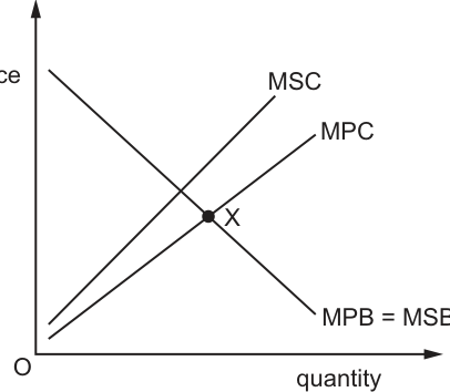
What should happen to achieve allocative efficiency?
Options
A a decrease in consumption and an increase in price
B a decrease in production and no change in price
C an increase in consumption and a decrease in production
D an increase in price and no change in production
Answer
The market equilibrium is at point X where marginal private benefit (MPB) equals marginal private cost (MPC). Allocative efficiency requires output where marginal social cost (MSC) equals marginal social benefit (MSB). Since MPB = MSB, efficiency requires MSC = MPB.
The diagram shows MSC to the left of MPC, indicating a negative externality of production (MSC > MPC). The intersection of MSC and MPB occurs at a lower quantity and a higher price than point X. Therefore, to achieve allocative efficiency, consumption must decrease and the price must increase.
A
A
Background Concept
Allocative efficiency is achieved when resources are allocated in a way that maximises societal welfare. This occurs where marginal social cost (MSC) equals marginal social benefit (MSB). At this point, the cost to society of producing the last unit equals the benefit to society from consuming it, and no net welfare gain is possible from reallocating resources.
When there is a negative externality of production, such as pollution, the marginal social cost exceeds the marginal private cost (MSC > MPC) because the producer does not bear the full cost of the external damage. The private market, ignoring this external cost, equates marginal private benefit (MPB) with marginal private cost (MPC), resulting in overproduction and overconsumption relative to the social optimum. The market equilibrium quantity is higher and the price lower than the socially optimal level. A deadweight welfare loss arises because units between the social optimum and the market equilibrium are produced for which MSC exceeds MSB.
Understanding the Question
The question presents a diagram with three curves: MPB (which equals MSB), MPC, and MSC. Point X marks the intersection of MPB and MPC, representing the unregulated private market equilibrium. The MSC curve is positioned to the left of the MPC curve, confirming a negative externality in production. The question asks what must happen to move from this private equilibrium to the point of allocative efficiency.
The command word "What should happen" requires identifying the directional change in price and consumption (quantity) necessary to reach the socially optimal outcome where MSC = MSB.
Approach
To answer this, first locate the socially efficient equilibrium: the intersection of the MSC and MSB (MPB) curves. Compare this point with the current private equilibrium at X. Because MSC lies above and to the left of MPC, the intersection with the downward-sloping MPB curve will be at a higher price and lower quantity than X. Therefore, the required adjustment is a decrease in consumption (and production) and an increase in price.
Step-by-Step Reasoning
- Identify the current equilibrium: Point X is where MPB = MPC. This is the free-market outcome.
- Identify the social optimum: Allocative efficiency requires MSC = MSB. Since MPB = MSB, we find where MSC intersects MPB.
- Analyse the curves: The MSC curve is to the left of MPC. In a price-quantity diagram, this means that at any given quantity, the social cost is higher than the private cost. Consequently, the MSC curve intersects the MPB curve at a point to the left of X (lower quantity) and above X (higher price).
- Determine the required changes: Moving from X to the socially optimal point requires reducing the quantity consumed and produced, and raising the price consumers pay to reflect the true social cost.
- Evaluate the options:
- Option A states a decrease in consumption and an increase in price. This matches the analysis.
- Option B is incorrect because price must rise, not stay unchanged.
- Option C is incorrect because consumption must fall, not rise.
- Option D is incorrect because production must fall, not stay unchanged.
- Conclusion: Option A is correct.
Key Takeaways
- Allocative efficiency is defined by the condition MSC = MSB.
- A negative production externality means MSC > MPC, causing the market to overproduce.
- Correcting this requires reducing output to the socially optimal level and raising the price to reflect the true social cost.
- In diagrammatic analysis, always compare the position of the social cost/benefit curves with the private curves to determine the direction of the necessary adjustment.
Common Mistakes
- Confusing the direction of price change: Some students might think that because the supply curve (MSC) shifts left or up, the price falls. However, with a downward-sloping demand curve, a leftward shift of the supply curve raises the equilibrium price.
- Misidentifying the curves: Confusing MPC with MSC or MPB with MSB can lead to comparing the wrong intersections.
- Ignoring the externality: Simply describing the private equilibrium without relating it to the social optimum fails to answer the question.
- Selecting options with no price change: Because the curves are not vertical or horizontal, both price and quantity must change to reach a new intersection of two curves.
Things to Be Careful About
- Ensure you read the diagram correctly: MSC to the left of MPC means higher costs at each quantity, not lower.
- Remember that allocative efficiency is about the social optimum (MSC = MSB), not the private optimum (MPC = MPB).
- The term "consumption" in the options refers to the quantity consumed, which equals the quantity produced in this simple model.
- In multiple-choice questions, eliminate options that maintain the status quo for either price or quantity, as moving to a new intersection of two curves generally changes both unless one curve is perfectly elastic or inelastic.
Firm X is considering whether to co-operate with its rival so that their joint profit is $4000 a month ($2000 each). It calculated that, if it did not co-operate, its own profit would be $2800 a month provided it kept all its customers itself. However, if its rival undercut X’s price and took some of X’s customers then X’s profit would be $1200. It has no knowledge of what the rival’s policy will be.
What describes the situation that the firm is facing?
Options
A monopoly profit maximisation
B principal agent problem
C prisoner’s dilemma
D satisficing
Reasoning
The scenario describes two firms where each has an incentive to act in its own self-interest (not co-operate) regardless of the other's action, leading to a lower joint profit than if they co-operated. This is the classic prisoner's dilemma in game theory.
Answer
C
C
Background Concept
The prisoner's dilemma is a standard game theory model used to analyse strategic behaviour in oligopoly. It shows that two rational, self-interested players may not co-operate even when co-operation would make them both better off. Each player has a dominant strategy — a strategy that yields the highest payoff regardless of what the other does. When both play their dominant strategy, the outcome is a Nash equilibrium that is worse for both than the co-operative outcome. In oligopoly, this explains why firms may engage in price wars or fail to collude even when collusion would raise joint profits.
Understanding the Question
Firm X is considering whether to co-operate with its rival. The payoffs are given: if both co-operate, each earns $2000. If X does not co-operate (defects) and the rival co-operates, X earns $2800. If the rival undercuts (defects) and X co-operates, X earns $1200. The rival's payoffs are symmetric but not fully stated. The question asks which economic concept describes this situation. The options are monopoly profit maximisation, principal-agent problem, prisoner's dilemma, and satisficing.
Approach
To identify the prisoner's dilemma, check for two features: (1) each player has a dominant strategy to defect, and (2) the outcome when both defect is worse for both than if both co-operate. Construct the payoff matrix mentally: if both co-operate, each gets $2000. If X defects and rival co-operates, X gets $2800 (higher than $2000), so defecting is better for X if the rival co-operates. If the rival defects, X's best response is also to defect (since $1200 is better than whatever X would get by co-operating when the rival defects, which would be even lower). Thus defecting is a dominant strategy for X. The same logic applies to the rival. The resulting outcome (both defect) gives each $1200, which is less than the $2000 from co-operation. This matches the prisoner's dilemma.
Step-by-Step Reasoning
- Identify the players: Firm X and its rival.
- Identify the strategies: co-operate (C) or not co-operate (defect, D).
- Payoffs for Firm X:
- If both C: $2000
- If X D and rival C: $2800
- If X C and rival D: $1200
- If both D: $1200 (implied, as the rival undercuts and X loses customers)
- For Firm X, compare payoffs:
- If rival C: D gives $2800 > C gives $2000, so D is better.
- If rival D: D gives $1200 > C gives (presumably less than $1200, e.g., $0 or negative), so D is better.
Thus D is a dominant strategy for X.
- By symmetry, D is also a dominant strategy for the rival.
- The dominant strategy equilibrium is (D, D) with payoffs ($1200, $1200).
- This is worse for both than (C, C) with ($2000, $2000).
- This structure is the prisoner's dilemma.
- Therefore, the correct answer is C.
Key Takeaways
- The prisoner's dilemma illustrates why oligopolistic firms may fail to collude even when collusion is mutually beneficial.
- A dominant strategy is one that is best regardless of the opponent's move.
- The outcome of the prisoner's dilemma is a Nash equilibrium that is Pareto inferior to the co-operative outcome.
- This concept is distinct from monopoly profit maximisation (single firm), principal-agent problem (conflict between owners and managers), and satisficing (aiming for satisfactory rather than maximum profit).
Common Mistakes
- Confusing the prisoner's dilemma with the principal-agent problem: the principal-agent problem involves asymmetric information and differing objectives between an owner and a manager, not strategic interaction between two firms.
- Thinking that the prisoner's dilemma requires explicit communication or a binding agreement; it does not — it is about incentives even without communication.
- Assuming that the dominant strategy is always to co-operate; in the prisoner's dilemma, the dominant strategy is to defect.
Things to Be Careful About
- Ensure the payoff structure clearly shows that defecting is dominant for both players and that the mutual defection outcome is worse than mutual co-operation.
- The question does not provide the rival's payoffs explicitly, but the symmetric nature of the scenario implies them.
- Do not overcomplicate: the description directly matches the classic prisoner's dilemma setup.
A smartphone manufacturing company takes over an electronic chip design company.
This is an example of which type of growth?
Options
A horizontal
B lateral
C vertical backwards
D vertical forwards
The smartphone manufacturer is acquiring a supplier of inputs (chip design), so the takeover is an example of backward vertical integration.
Answer
C
C
Background Concept
Firms can grow externally by integrating with other firms through mergers or takeovers. The main types are:
- Horizontal integration: firms at the same stage of production in the same industry (e.g., two smartphone manufacturers merging).
- Vertical integration: firms at different stages of the same supply chain. If the firm acquires a supplier, it is backward vertical integration; if it acquires a distributor or retailer, it is forward vertical integration.
- Lateral integration: firms in different but related industries (e.g., a smartphone maker buying a software developer that complements its products).
Understanding the Question
The question describes a smartphone manufacturing company taking over an electronic chip design company. Chips are an input into smartphones, so the target is a supplier. This is a move 'backward' along the supply chain. The options require one to distinguish which type of external growth is happening.
Approach
Identify the position of the acquired firm relative to the acquiring firm in the chain from raw materials to final consumer. If it is a supplier, it is backward; if a distributor, forward; if a direct competitor, horizontal; if a related but different market, lateral.
Step-by-Step Reasoning
- The smartphone producer assembles final phones.
- Chips are a component used in production.
- A chip design company supplies these chips (or designs them for manufacture) — it is earlier in the supply chain.
- Therefore the takeover is vertical and backwards.
- Option A (horizontal) would be if the target were another smartphone manufacturer. Option B (lateral) might be if the target made something complementary but not directly a supplier (e.g., phone cases). Option D (vertical forwards) would be if the target distributed or sold the smartphones to final consumers.
- So only option C fits.
Key Takeaways
- Learn the four standard directions of integration: horizontal, vertical backwards, vertical forwards, and lateral (sometimes called conglomerate if unrelated).
- Always identify the relationship between the acquiring and acquired firm: supplier, customer, competitor, or unrelated.
- Backward integration secures supply of inputs; forward integration secures distribution channels.
Common Mistakes
- Confusing backwards and forwards: think of the flow of goods — if the acquired firm supplies inputs, the acquirer is moving 'back' along the chain. If it sells the final product, it is moving 'forward'.
- Thinking 'vertical' only means 'different stages' without checking direction — the question specifically asks which type, so direction matters.
- Selecting 'lateral' when the firms are in the same broad industry but not in a direct supplier-customer relationship; here they are definitely in a supplier relationship.
Things to Be Careful About
- The description says 'takes over an electronic chip design company' — a chip design company may not physically manufacture chips, but it still supplies intellectual property or designs that are inputs to production. That is enough to be a supplier.
- Some questions might use different wording (e.g., 'backward' vs 'backwards') — both are acceptable, but option C uses 'vertical backwards'.
- The mark scheme answer is C, so always check the exact label used in the options.
What is not a valid comment economists may make regarding the need to subsidise a green energy market that uses solar and wind power?
Options
A It is cheaper to use the plentiful supply of coal.
B Markets will become more efficient.
C The value of the positive externalities cannot be estimated.
D The value of the negative externalities cannot be estimated.
Reasoning
The need to subsidise green energy arises from positive externalities (benefits to society not captured by private producers). A subsidy can internalise the externality and improve allocative efficiency. However, the statement 'Markets will become more efficient' is not a valid comment regarding the need to subsidise because it is a potential outcome, not a reason for the subsidy. Moreover, the subsidy itself may introduce inefficiencies (government failure), so the claim is not necessarily true. The other options are valid comments: A points to the cost advantage of coal (though ignoring externalities), C and D highlight the difficulty in estimating externalities, which are genuine concerns.
Answer
B
B
Background Concept
This question tests understanding of market failure due to externalities and the role of government intervention through subsidies. Green energy (solar and wind) generates positive externalities: it reduces carbon emissions, improves air quality, and enhances energy security, benefits that are not reflected in the market price. Without intervention, the market underproduces green energy relative to the socially optimal level. A subsidy can lower the private cost of production, encouraging more output and moving the market closer to allocative efficiency. However, subsidies also have drawbacks: they require government revenue (often from distortionary taxes), may lead to overproduction if set too high, and can create government failure.
Understanding the Question
The question asks which of four statements is NOT a valid comment that economists might make about the need to subsidise a green energy market. It requires distinguishing between comments that are economically sound (even if debatable) and those that are not. The correct answer is B: 'Markets will become more efficient.' This statement is not a valid comment because it is ambiguous and not necessarily true; the subsidy could improve efficiency if correctly targeted, but it could also cause inefficiency. The other options are all valid comments that economists might raise in a discussion about the need for subsidy.
Approach
Evaluate each option in turn:
- A: 'It is cheaper to use the plentiful supply of coal.' This is a valid comment because it points to the private cost advantage of coal, though it ignores externalities. Economists might use this to argue against subsidy, but it is a valid observation.
- B: 'Markets will become more efficient.' This is not a valid comment because the market is currently inefficient due to externalities; a subsidy can improve efficiency, but the statement is too broad and does not address the need. Also, the subsidy might not make markets more efficient if it leads to government failure.
- C: 'The value of the positive externalities cannot be estimated.' This is a valid comment: quantifying externalities is difficult, so setting the optimal subsidy is challenging.
- D: 'The value of the negative externalities cannot be estimated.' Similarly valid: negative externalities from fossil fuels are hard to measure, complicating the case for subsidy.
Thus, B is the only option that is not a valid comment.
Step-by-Step Reasoning
-
Option A: 'It is cheaper to use the plentiful supply of coal.' Economists might say this to highlight that without subsidy, coal is cheaper, so green energy needs subsidy to compete. However, this comment ignores the negative externalities of coal (pollution, health costs). Still, it is a valid comment because it reflects a real cost comparison. It is a comment about the need for subsidy to level the playing field.
-
Option B: 'Markets will become more efficient.' This statement is problematic. The market for green energy is already inefficient because of positive externalities. A subsidy can correct this and improve allocative efficiency. However, the statement as phrased is not a comment about the need for subsidy; it is a claim about the outcome. Moreover, economists would not assert that markets will definitely become more efficient because the subsidy itself may create inefficiencies (e.g., deadweight loss from taxation, overproduction). Therefore, this is not a valid comment to make regarding the need to subsidise.
-
Option C: 'The value of the positive externalities cannot be estimated.' This is a valid comment. It points to a practical difficulty in implementing the subsidy: if the external benefit cannot be quantified, the subsidy may be set at the wrong level, leading to suboptimal outcomes. This is a common economic argument against intervention.
-
Option D: 'The value of the negative externalities cannot be estimated.' Similarly valid. The negative externalities from fossil fuels (e.g., climate change) are hard to measure, so the case for subsidising green energy as a substitute is weakened by uncertainty. This is a valid comment.
Therefore, only B is not a valid comment.
Key Takeaways
- Subsidies are used to correct positive externalities by lowering private costs and increasing output toward the social optimum.
- Economists consider both the benefits and costs of intervention, including the difficulty of measuring externalities and the risk of government failure.
- When evaluating statements about economic policy, distinguish between reasons for intervention, potential outcomes, and practical challenges.
Common Mistakes
- Assuming that any statement that sounds economic is automatically valid. Option B might seem plausible, but it is not a valid comment about the need to subsidise because it is a vague claim about efficiency.
- Ignoring the possibility of government failure: subsidies can lead to inefficiency if poorly designed.
- Overlooking that options A, C, and D are all valid comments that economists might make, even if they are not the only considerations.
Things to Be Careful About
- Read the question carefully: 'not a valid comment' means the statement is not an economically sound comment to make in this context.
- Understand that 'valid' here means 'economically reasonable', not 'true' or 'correct'. All options except B are reasonable comments that economists might raise.
- Remember that externalities are a key reason for government intervention, but the difficulty of measurement is a valid concern.
In which situation is the introduction of a minimum wage most likely to raise employment opportunities as well as wages?
Options
A Firms face intense competition both at home and abroad.
B Labour costs are a high proportion of the total cost of the firm.
C The minimum wage is not high enough to lower the profits of the firms.
D The minimum wage introduced in monopsony is less than the marginal revenue productivity (MRP) of the last worker employed.
Answer
In a monopsony labour market, the employer has market power and pays a wage below the marginal revenue product (MRP) of labour. A minimum wage set between the monopsony wage and the MRP of the last worker employed can raise both wages and employment. This is because the minimum wage makes the supply of labour perfectly elastic up to the point where it intersects the labour supply curve, allowing the firm to hire more workers at the higher wage. Option D describes this condition.
D
Background Concept
In a perfectly competitive labour market, the wage is determined by supply and demand. A minimum wage above the equilibrium leads to a surplus of labour (unemployment). However, in a monopsony labour market, there is a single buyer of labour (e.g., a dominant employer in a town). The monopsonist faces an upward-sloping supply curve of labour, meaning to hire more workers, it must raise the wage for all workers. This makes the marginal cost of labour (MCL) greater than the wage. The monopsonist hires labour where MCL equals the marginal revenue product (MRP) of labour, and pays a wage determined by the supply curve at that employment level. This results in a wage lower than the MRP and lower employment than in a competitive market.
Understanding the Question
The question asks for the situation where a minimum wage can increase both wages and employment. This is counterintuitive because the standard model predicts a minimum wage reduces employment. The key is to recognise that in a monopsony, the initial wage is below the competitive level, and a carefully set minimum wage can move the market closer to the competitive outcome, increasing both wage and employment. Option D correctly identifies the condition: the minimum wage is less than the MRP of the last worker employed. This ensures that the minimum wage does not exceed the value of the worker's output, so the firm can profitably hire more workers.
Approach
To answer, we need to recall the monopsony model and the effect of a minimum wage. We can analyse the labour market diagrammatically or logically. The correct option is D because it describes the monopsony condition that allows employment to rise. The other options do not capture the necessary market structure or condition.
Step-by-Step Reasoning
- In a monopsony, the firm's MCL curve lies above the supply curve. The firm hires where MCL = MRP, at employment Lm, and pays wage Wm (from the supply curve at Lm). At Lm, MRP > Wm.
- If a minimum wage Wmin is imposed such that Wm < Wmin < MRP at Lm, then the supply of labour becomes perfectly elastic at Wmin up to the point where the supply curve reaches Wmin. The MCL becomes constant at Wmin up to that intersection.
- The firm now hires where the new MCL (Wmin) equals MRP. Since Wmin is less than the original MRP at Lm, the MRP at a higher employment level will be lower (due to diminishing returns). The firm will increase employment until MRP = Wmin.
- Thus, both the wage (from Wm to Wmin) and employment (from Lm to Lmin) increase.
- Option D states that the minimum wage is less than the MRP of the last worker employed. This is exactly the condition that allows employment to rise. If the minimum wage were above MRP, the firm would reduce employment.
Key Takeaways
- Minimum wage can increase employment in a monopsony labour market.
- The condition is that the minimum wage is set between the monopsony wage and the MRP of the last worker.
- This result highlights the importance of market structure in policy analysis.
Common Mistakes
- Assuming minimum wage always reduces employment without considering market structure.
- Confusing MRP with the wage; MRP is the additional revenue from hiring one more worker.
- Thinking that any minimum wage in monopsony increases employment; it must be below MRP.
Things to Be Careful About
- The phrase "last worker employed" refers to the monopsony employment level.
- The minimum wage must be less than the MRP at that point; if it exceeds MRP, employment falls.
- The analysis assumes the firm is a profit-maximising monopsonist.
The diagram shows a firm’s initial marginal revenue product of labour curve (MRP1).
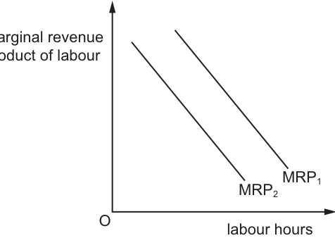
What could cause the curve to shift to MRP2?
Options
A a fall in the wage rate
B a fall in the price of the final product
C a rise in the wage rate
D a rise in the price of the final product
Working
The marginal revenue product of labour (MRP) is calculated as MRP = marginal revenue (MR) × marginal product of labour (MP). A shift of the entire MRP curve occurs when either MR or MP changes, while a change in the wage rate (the cost of labour) causes a movement along the existing MRP curve.
- A fall in the wage rate (A) and a rise in the wage rate (C) change the quantity of labour demanded, leading to a movement along the MRP curve, not a shift.
- A rise in the price of the final product (D) increases MR, so MRP rises at every level of labour, shifting the curve rightward (to the right of MRP1).
- A fall in the price of the final product (B) reduces MR, so MRP falls at every level of labour, shifting the curve leftward to MRP2 as shown.
Answer
B
B
Background Concept
Marginal revenue product of labour (MRP) is a core concept in labour demand theory, measuring the additional revenue a firm earns from employing one extra unit of labour. It is calculated using the formula MRP = marginal revenue (MR, the extra revenue from selling one more unit of the final good) × marginal product of labour (MP, the extra output from one more unit of labour). The MRP curve is normally downward sloping due to the law of diminishing marginal returns: as more labour is employed with other factors fixed, MP falls, so MRP falls at higher employment levels. A critical distinction in this topic is between a shift of the entire MRP curve and a movement along it: a shift occurs when a non-wage factor changes MR or MP, while a change in the wage rate (the price of labour) only changes the quantity of labour the firm chooses to demand, causing a movement along the existing curve.
Understanding the Question
The question provides a diagram showing two parallel downward-sloping MRP curves: MRP1 (the initial curve) and MRP2, which is shifted leftward. A leftward shift means that at every level of labour hours, the marginal revenue product of labour is lower than before. The question asks which of the four options causes this specific leftward shift. The options include two wage rate changes (A and C) and two final product price changes (B and D). The question tests two linked skills: knowing what shifts the MRP curve, and understanding how changes in final product price affect MR and thus MRP.
Approach
To solve this, first recall the MRP formula and the difference between curve shifts and movements along the curve. First eliminate the wage rate options, as wage changes affect the quantity of labour demanded, not the MRP itself. Then evaluate the two price options: a rise in final product price increases MR and shifts MRP right, while a fall reduces MR and shifts MRP left. Match this to the diagram's leftward shift to identify the correct answer.
Step-by-Step Reasoning
- Start with the core MRP relationship: MRP = MR × MP. Any change that alters MR or MP will shift the entire MRP curve, while a change in the wage rate only changes the quantity of labour demanded, causing a movement along the existing curve.
- Evaluate options A and C: A fall in the wage rate (A) makes labour cheaper, so the firm demands more labour, moving down along the MRP curve. A rise in the wage rate (C) makes labour more expensive, so the firm demands less labour, moving up along the MRP curve. Neither option shifts the curve itself, so both are incorrect.
- Evaluate option D: A rise in the price of the final product increases the marginal revenue the firm earns from each additional unit of output. With higher MR, MRP rises at every level of labour employment, shifting the MRP curve rightward (to the right of MRP1). This is the opposite of the shift shown in the diagram, so D is incorrect.
- Evaluate option B: A fall in the price of the final product reduces the marginal revenue the firm earns from each additional unit of output. With lower MR, MRP falls at every level of labour, so the entire MRP curve shifts leftward to MRP2, exactly matching the diagram. This is the correct cause.
Key Takeaways
- MRP depends on both MR and MP, so it shifts only when either of these two variables changes.
- Changes in the wage rate cause movements along the MRP curve, not shifts of the curve.
- A leftward shift of the MRP curve means MRP is lower at every level of employment, which occurs when MR falls (e.g. lower final product price) or MP falls (e.g. lower labour productivity).
- Always distinguish between a shift of a curve (caused by a non-price determinant of the vertical axis variable) and a movement along the curve (caused by a change in the vertical axis variable or the price of the factor being demanded).
Common Mistakes
- Confusing movements along the MRP curve with shifts: many students incorrectly select a wage rate change as the cause of a shift, but wage changes only affect the quantity of labour demanded, not the MRP itself.
- Reversing the direction of the price effect: a rise in final product price increases MR and shifts MRP right, while a fall shifts it left. Students often mix up this relationship.
- Forgetting the MRP formula: without recalling that MRP depends on both MP and MR, it is impossible to identify what shifts the curve.
Things to Be Careful About
- The wage rate is the cost of labour, not a determinant of MRP itself. MRP measures the revenue the firm generates from labour, not the cost of hiring it.
- The diagram shows a parallel leftward shift, which indicates the entire MRP falls at every level of labour with no change in the slope of the curve. This is consistent with a fall in MR (with MP unchanged), rather than a fall in MP (which would make the curve steeper).
- Always check the direction of the shift in the diagram: leftward = lower MRP at every quantity, rightward = higher MRP at every quantity, to avoid selecting the wrong price option.
A firm operates in a perfectly competitive labour market.
The table shows the marginal revenue product (MRP) and marginal cost of labour (MCL) for each additional worker employed by this profit-maximising firm.
| units of labour employed | MRP | MCL |
|---|---|---|
| 1 | 50 | 30 |
| 2 | 40 | 30 |
| 3 | 30 | 30 |
| 4 | 20 | 30 |
How many units of labour will this firm employ?
Options
A 1
B 2
C 3
D 4
Reasoning
A profit-maximising firm in a perfectly competitive labour market will hire workers up to the point where the marginal revenue product (MRP) equals the marginal cost of labour (MCL). From the table:
- Worker 1: MRP = 50, MCL = 30 → MRP > MCL, hire.
- Worker 2: MRP = 40, MCL = 30 → MRP > MCL, hire.
- Worker 3: MRP = 30, MCL = 30 → MRP = MCL, hire.
- Worker 4: MRP = 20, MCL = 30 → MRP < MCL, do not hire.
Thus, the firm will employ 3 workers.
Answer
C
C
Background Concept
In a perfectly competitive labour market, the firm is a wage taker, meaning it can hire any number of workers at the market wage rate. The marginal cost of labour (MCL) is constant and equal to the wage rate. The firm's demand for labour is derived from the marginal revenue product (MRP), which is the additional revenue generated by hiring one more worker. MRP is calculated as marginal product (MP) times marginal revenue (MR). For a profit-maximising firm, the optimal level of employment is where MRP = MCL. If MRP > MCL, the firm can increase profit by hiring more workers; if MRP < MCL, the firm should reduce employment. The firm will hire the last worker for which MRP is at least equal to MCL.
Understanding the Question
This question provides a table showing the MRP and MCL for each additional worker employed by a firm in a perfectly competitive labour market. The firm is profit-maximising. We are asked to determine how many units of labour the firm will employ. The table lists four workers with their respective MRP and MCL values. The correct answer is the number of workers that satisfies the profit-maximising condition.
Approach
We compare MRP and MCL for each worker sequentially. Starting from the first worker, we check if MRP >= MCL. If yes, the worker is hired. We continue until we encounter a worker where MRP < MCL, at which point we stop. The number of workers hired is the last one for which MRP >= MCL.
Step-by-Step Reasoning
- For worker 1: MRP = 50, MCL = 30. Since 50 > 30, hiring this worker adds more to revenue than to cost, increasing profit. So the firm hires worker 1.
- For worker 2: MRP = 40, MCL = 30. Again, 40 > 30, so hiring worker 2 also increases profit. The firm hires worker 2.
- For worker 3: MRP = 30, MCL = 30. Here MRP equals MCL, so hiring worker 3 adds exactly as much to revenue as to cost. The firm is indifferent, but in standard profit-maximising theory, the firm will hire this worker because it does not reduce profit. So the firm hires worker 3.
- For worker 4: MRP = 20, MCL = 30. Since 20 < 30, hiring worker 4 would reduce profit. The firm will not hire worker 4.
Thus, the firm employs 3 workers.
Key Takeaways
- The profit-maximising rule for hiring labour is MRP = MCL in a perfectly competitive labour market.
- When MRP > MCL, the firm should hire more workers; when MRP < MCL, it should hire fewer.
- The optimal number of workers is the last one for which MRP is at least equal to MCL.
- This rule is analogous to the profit-maximising output rule (MC = MR).
Common Mistakes
- Hiring the worker where MRP is highest (worker 1) without considering the marginal cost. The firm must compare MRP with MCL, not just look at MRP.
- Hiring all workers where MRP > MCL but stopping before MRP = MCL. In this case, worker 3 has MRP = MCL, so it should be included.
- Confusing MCL with the wage rate. In perfect competition, MCL is constant and equal to the wage, but the rule is still MRP = MCL.
- Thinking that the firm should hire until MRP is zero or until MRP is maximised. The correct criterion is equality at the margin.
Things to Be Careful About
- Ensure you compare MRP and MCL for each worker sequentially, not just the total.
- Remember that the firm is profit-maximising, not revenue-maximising or cost-minimising.
- In perfect competition, the MCL is constant, but in other market structures (e.g., monopsony), MCL may increase with employment. This question specifies perfect competition, so MCL is constant.
- The table gives MRP and MCL for each additional worker, so we use marginal analysis.
Countries in South East Asia have some of the highest income inequality in the world.
Which policy could be adopted by governments in South East Asia to reduce income inequality in the short run?
Options
A Increase the general sales tax /VAT rate on luxury goods.
B Introduce a minimum wage.
C Invest heavily in schools and education programmes.
D Stimulate economic growth through skills and productivity training.
Answer
A minimum wage directly raises the wages of low-income workers, increasing their income relative to higher-income earners, thus reducing income inequality in the short run. The other options (A, C, D) are either ineffective in the short run or take longer to have an impact.
Answer
B
B
Background Concept
Income inequality refers to the disparity in the distribution of income among individuals or households. It is often measured using the Gini coefficient. Policies to reduce income inequality can be classified as short-run or long-run in their impact. Short-run policies directly alter the distribution of income quickly, such as minimum wage laws, tax and transfer systems, and price controls. Long-run policies aim to change the underlying determinants of income, such as education, training, and economic growth, which take time to materialise.
Understanding the Question
The question asks: "Which policy could be adopted by governments in South East Asia to reduce income inequality in the short run?" The key phrase is "in the short run". This means the policy should have an immediate effect on the distribution of income, not one that takes years to work through the economy. The four options are:
- A: Increase the general sales tax / VAT rate on luxury goods.
- B: Introduce a minimum wage.
- C: Invest heavily in schools and education programmes.
- D: Stimulate economic growth through skills and productivity training.
Approach
To answer, we need to evaluate each option by its time horizon. Ask: Does this policy raise the incomes of low-income earners quickly (within months or a year) or does it require years to affect income? Minimum wage is a direct intervention that raises the wages of low-paid workers as soon as it is implemented. Tax changes on luxury goods may have some effect but are not a direct transfer to the poor and may be regressive. Education and skills training are long-term investments that take time to improve human capital and earnings.
Step-by-Step Reasoning
-
Option A: Increase the general sales tax / VAT rate on luxury goods. Luxury goods are items consumed disproportionately by higher-income individuals. A higher tax on these goods might reduce the disposable income of the rich, but it does not directly increase the income of the poor. Moreover, the tax could be passed on to consumers in the form of higher prices, and if low-income earners also purchase some luxury goods, they may be hurt. The effect on inequality is uncertain and not immediate; it is not a short-run solution.
-
Option B: Introduce a minimum wage. A minimum wage sets a floor on wages. It directly increases the earnings of low-paid workers, many of whom are in the lower tail of the income distribution. This raises their income relative to higher-income earners, thereby reducing income inequality. The effect is immediate: as soon as the law is enforced, wages for covered workers rise. Even if there is some disemployment effect (some workers may lose jobs), the overall impact on inequality is likely to be positive in the short run because the income of those who remain employed increases. This is the correct answer.
-
Option C: Invest heavily in schools and education programmes. Education improves human capital, leading to higher productivity and earnings in the long run. However, it takes years to complete schooling and for the labour market to reward the new skills. This is a long-run policy, not a short-run one.
-
Option D: Stimulate economic growth through skills and productivity training. Similar to education, this aims to increase the productive capacity of the economy. It may eventually raise wages, but the process takes time. The training itself takes time, and the benefits accrue only after workers apply their new skills. Again, this is a long-run policy.
Therefore, only option B can reduce income inequality in the short run.
Key Takeaways
- Short-run policies to reduce inequality directly affect income distribution (e.g., minimum wage, tax credits, transfers).
- Long-run policies focus on human capital and economic growth; they take time to have an effect.
- Minimum wage is a direct tool that can quickly raise the incomes of low-paid workers, but it may also have negative side effects such as unemployment, which should be considered in a full evaluation.
Common Mistakes
- Confusing short-run and long-run effects: students may think that education or training can reduce inequality quickly, but they take years to materialise.
- Assuming that taxing luxury goods is an effective way to reduce inequality: it may reduce the disposable income of the rich, but it does not directly help the poor and could be regressive if the poor consume some luxury goods.
- Overlooking the time horizon: the question explicitly says "in the short run", so any policy that requires time to work (like education) is incorrect.
Things to Be Careful About
- The question is about income inequality, not about poverty or employment. Minimum wage directly affects the distribution of labour income, which is a major component of total income.
- In the short run, even if minimum wage causes some job losses, the income of those who keep their jobs rises, and the overall effect on the Gini coefficient could be positive. However, this is a nuance; the main point is that it is the only option with an immediate effect.
- Be precise with the term "short run": in economics, it means at least one period where some factors are fixed. For policy, it means the effect is felt within a few months to a year, not years later.
When buying a car, Salma agrees to pay half of the cost now and the other half in six months time.
Which function of money does this illustrate?
Options
A divisibility
B durability
C standard of deferred payment
D store of value
Reasoning
Money serves four main functions: a medium of exchange, a unit of account, a store of value, and a standard of deferred payment. The scenario describes Salma agreeing to pay half the cost now and the other half in six months' time. This involves a promise to pay in the future, which is the essence of the standard of deferred payment function. Money is used as a standard for settling debts that are payable at a future date.
Divisibility (A) refers to the ability to divide money into smaller units. Durability (B) refers to the physical longevity of money. Store of value (D) refers to the ability of money to retain its purchasing power over time. None of these directly describe the transaction in the question.
Answer
C
C
Background Concept
Money is traditionally defined by four key functions:
- Medium of exchange: Money is widely accepted in exchange for goods and services, eliminating the need for barter.
- Unit of account: Money provides a common measure of value, allowing prices to be quoted and accounts to be kept.
- Store of value: Money allows purchasing power to be transferred from the present to the future. It must hold its value over time (though inflation can erode it).
- Standard of deferred payment: Money facilitates credit transactions by providing a means to settle debts that are payable in the future. It is the yardstick for future payments.
Understanding the Question
The question presents a specific scenario: Salma agrees to pay half the cost of a car now and the other half in six months. The task is to identify which function of money is being illustrated by this arrangement. The answer requires distinguishing between the four functions and applying them to real-world credit transactions.
Approach
Consider each function in turn and test whether it matches the scenario. The key element is the delayed payment component. The scenario involves a credit agreement where payment is deferred. The function that directly relates to the use of money in credit transactions is the standard of deferred payment. The other functions, while important, do not capture the essence of paying later.
Step-by-Step Reasoning
-
Divisibility: Money can be divided into smaller units (e.g., pounds into pence, dollars into cents). This is useful for making change but not relevant to the agreement to pay half now and half later. The scenario does not involve dividing money into smaller denominations.
-
Durability: Money must be physically durable so it can be used repeatedly. This is a physical characteristic, not related to the timing of payments. The scenario is about the timing of payment, not the physical quality of money.
-
Store of value: Money can be saved and used later because it retains its value over time (ignoring inflation). If Salma pays half now, the seller is accepting the first half now and the second half as a future payment. The seller is using money as a store of value by accepting the promise of future payment, but the emphasis is on the contractual promise to pay later, not on the store of value function per se. The store of value function is about holding money, not about using it to settle debts.
-
Standard of deferred payment: Money is used as a standard for future payments. When a buyer agrees to pay later, the debt is denominated in money. The amount is fixed in monetary terms, and the future payment will be made in money. This is precisely what happens with Salma: she agrees to pay a specific monetary amount in six months. The transaction relies on money being the accepted standard for settling debts over time.
Therefore, the correct answer is C: standard of deferred payment.
Key Takeaways
- The four functions of money are distinct and each applies to different aspects of economic life.
- The standard of deferred payment function is specifically about the use of money in credit and debt contracts.
- When a question involves a promise to pay in the future, the relevant function is almost always standard of deferred payment.
Common Mistakes
- Confusing store of value with standard of deferred payment: Both involve time, but store of value is about holding money as an asset, while standard of deferred payment is about denominating debts that will be paid later. In this scenario, the agreement to pay later is a credit arrangement, not simply holding money.
- Choosing divisibility because the payment is split: The question mentions "half" which might lead some to think of divisibility. But divisibility is about the physical ability to make change, not about splitting a payment over time.
Things to Be Careful About
- Read the scenario carefully: look for the key phrase "pay the other half in six months time" — that indicates a future payment obligation.
- Remember that the four functions are defined in terms of what money does in the economy. The standard of deferred payment is the only one that directly involves the use of money to settle future debts.
When is the natural rate of unemployment most likely to fall?
Options
A when there is a decline in the education levels of workers
B when there is an increase in income tax rates
C when there is an increase in labour mobility
D when there is a rise in the rate of state unemployment benefits
Reasoning
The natural rate of unemployment consists of frictional and structural unemployment at equilibrium in the labour market, when cyclical unemployment is zero. An increase in labour mobility (C) allows workers to move more easily between jobs, occupations and regions, reducing the time spent searching for a new job (frictional unemployment) and helping to match skills with vacancies (structural unemployment). This directly lowers the natural rate.
A decline in education levels (A) worsens the mismatch between workers' skills and available jobs, increasing structural unemployment and raising the natural rate. Higher income tax rates (B) reduce the net reward from work, potentially lowering labour force participation and increasing the natural rate as some workers withdraw. A rise in state unemployment benefit rates (D) reduces the opportunity cost of remaining unemployed, lengthening job search and increasing frictional unemployment, which raises the natural rate.
Answer
C
C
Background Concept
The natural rate of unemployment is the rate of unemployment that exists when the labour market is in equilibrium — that is, when the number of job seekers equals the number of job vacancies and there is no cyclical (demand-deficient) unemployment. It consists of:
- Frictional unemployment: unemployment arising from the time workers spend searching for new jobs (e.g., graduates looking for their first role, people moving between jobs).
- Structural unemployment: unemployment caused by a mismatch between the skills or location of workers and the requirements of available jobs (e.g., an industry declining while a different industry grows, requiring retraining or relocation).
The natural rate is determined by factors that affect the efficiency of the labour market: labour mobility, the quality of information about vacancies, the level of unemployment benefits, training and education, tax and benefit systems, and the degree of trade union power or regulation. Policies aimed at reducing the natural rate focus on making the labour market work more smoothly — reducing frictions and improving matching.
Understanding the Question
The question asks: "When is the natural rate of unemployment most likely to fall?" A single correct option describes a change that would reduce frictional and/or structural unemployment. Three other options describe changes that would either increase these types of unemployment or have ambiguous effects. The candidate must evaluate each option against the definition and determinants of the natural rate.
Approach
Identify the component of the natural rate (frictional or structural) that each option affects, then judge whether the change would increase or decrease that component. Eliminate the options that would raise the natural rate, and select the one that would lower it.
Step-by-Step Reasoning
-
Option C — Increase in labour mobility: Labour mobility refers to the ease with which workers can move between jobs, occupations, and geographical areas. Higher mobility reduces the time spent in frictional unemployment (workers find new jobs faster) and reduces structural unemployment (workers can relocate or retrain more easily to fill vacancies in growing sectors). This clearly lowers the natural rate. Therefore C is correct.
-
Option A — Decline in education levels of workers: Education improves workers' skills and their ability to adapt to new jobs. A decline in education levels worsens the skills mismatch between workers and available jobs, increasing structural unemployment. This raises the natural rate, so A is not a cause of a fall.
-
Option B — Increase in income tax rates: Higher taxes reduce the net wage from work. Theoretical and empirical evidence suggests this can reduce labour supply (some workers leave the labour force or choose not to work as many hours) and increase the natural rate as the opportunity cost of not working falls. However, the effect is complex and may be small; the key point is that it does not lower the natural rate. Some economists argue it can increase the natural rate, but it certainly does not reduce it.
-
Option D — Rise in the rate of state unemployment benefits: Generous unemployment benefits reduce the opportunity cost of staying unemployed (the cost of not working is lower because benefit income substitutes for lost wages). This lengthens job search duration, increasing frictional unemployment and the natural rate. This is a well-established determinant in both theory and empirical work.
Only option C points in the direction of a lower natural rate.
Key Takeaways
- The natural rate of unemployment is the sum of frictional and structural unemployment at labour market equilibrium.
- Anything that improves the matching of workers to jobs — such as higher labour mobility, better information, retraining programmes, or job-search assistance — reduces the natural rate.
- Policies that raise the opportunity cost of work (higher taxes, higher benefits, less education) tend to increase the natural rate.
- This question tests understanding of the determinants of the natural rate rather than short-run cyclical changes.
Common Mistakes
- Confusing the natural rate with the actual or cyclical rate of unemployment. The natural rate is not affected by aggregate demand fluctuations in the long run.
- Thinking that higher unemployment benefits reduce unemployment (some might argue it reduces poverty). But the economic effect is to increase frictional unemployment and thus the natural rate.
- Assuming education is only about productivity; while education raises productivity, the direct effect on the natural rate works through reducing structural mismatch.
- Overcomplicating the tax option: the expected direction is that higher taxes reduce work incentives, raising the natural rate, so it cannot be the answer.
Things to Be Careful About
- Distinguish between the natural rate and cyclical/demand-deficient unemployment. The question is specifically about the natural rate.
- Labour mobility includes occupational, geographical, and industrial mobility. All reduce both frictional and structural unemployment.
- The term "most likely" implies we are selecting the option that unambiguously reduces the natural rate; the other options unambiguously increase it or at least do not decrease it.
- Be precise in reasoning: link each option to a specific type of unemployment (frictional or structural) that forms the natural rate.
A country has increasing productivity and falling unemployment.
What can be concluded from this information?
Options
A Economic efficiency has increased.
B Interest rates have increased.
C Taxation has increased.
D The labour force has increased.
Answer
Rising productivity means more output is produced per unit of input, which indicates an improvement in productive efficiency. Falling unemployment means more of the economy's labour resources are being used, which also contributes to a more efficient allocation of resources. Together, these two observations point to an overall increase in economic efficiency.
Option A is therefore correct.
Options B, C, and D are not necessarily implied by the given information. Interest rates could be rising or falling independently; taxation could be changing for reasons unrelated to productivity or unemployment; and a larger labour force would not, by itself, cause both rising productivity and falling unemployment — indeed, a larger labour force could increase unemployment if jobs are not created fast enough.
A
Background Concept
Economic efficiency has two main dimensions:
- Productive efficiency: producing goods and services at the lowest possible cost per unit, i.e., on the production possibility frontier (PPF). Rising productivity — more output per worker or per unit of capital — is a direct sign of improving productive efficiency.
- Allocative efficiency: resources are distributed to produce the combination of goods and services that society most values. Falling unemployment means more labour resources are being used, which moves the economy closer to its PPF (closing a negative output gap) and can improve allocative efficiency if the newly employed workers are producing goods that are in demand.
Together, rising productivity and falling unemployment suggest the economy is producing more output from its available resources — a clear improvement in economic efficiency.
Understanding the Question
The question presents two factual observations about a country: productivity is rising, and unemployment is falling. It asks what can be concluded from this information — i.e., which of the four options is a necessary or highly likely consequence, not merely a possible one. The command word "concluded" demands a logical inference, not speculation.
Approach
Evaluate each option against the given facts:
- Option A: Does rising productivity + falling unemployment necessarily imply increased economic efficiency? Yes — both facts point to better use of resources.
- Option B: Could interest rates have increased? Possibly, but not necessarily. The facts don't tell us about monetary policy.
- Option C: Could taxation have increased? Again, possible but not necessary.
- Option D: Could the labour force have increased? A larger labour force would tend to increase unemployment (more people seeking work), not reduce it, unless job creation is even faster. The given facts don't support this conclusion.
Step-by-Step Reasoning
-
Productivity is rising: This means each worker (or unit of capital) produces more output per time period. This is a direct measure of productive efficiency — the economy is getting more output from the same inputs.
-
Unemployment is falling: Fewer workers are without jobs. This means more of the available labour supply is being utilised, moving the economy closer to its full-employment level of output (potential GDP). This reduces any negative output gap and improves allocative efficiency (resources are less wasted).
-
Combined implication: Both trends point in the same direction — the economy is producing more output from its resources. This is the definition of increased economic efficiency. Option A is the only logical conclusion.
-
Why not B (interest rates increased)? Higher interest rates typically reduce investment and consumption, which could lower output and employment — the opposite of what is observed. While it's possible that interest rates rose for other reasons (e.g., to control inflation) and the economy still grew, this is not a necessary conclusion from the given facts.
-
Why not C (taxation increased)? Higher taxes generally reduce disposable income and aggregate demand, which could reduce output and employment. Again, not a necessary conclusion.
-
Why not D (labour force increased)? A larger labour force means more people are either employed or actively seeking work. If the labour force grows faster than employment, unemployment would rise, not fall. The given facts show falling unemployment, which is inconsistent with a rapidly expanding labour force (unless job creation is even faster, but that's an additional assumption not given).
Key Takeaways
- Rising productivity is a direct indicator of improving productive efficiency.
- Falling unemployment indicates better utilisation of labour resources, moving the economy toward its PPF.
- Together, these two observations strongly suggest an overall increase in economic efficiency.
- Be careful not to infer other macroeconomic changes (interest rates, taxation, labour force size) unless they are logically necessary from the given information.
Common Mistakes
- Confusing correlation with causation: A student might think that because productivity and unemployment are both improving, some other variable (like interest rates or taxation) must have caused it. But the question asks what can be concluded, not what might have caused it.
- Overlooking the definition of economic efficiency: Some students might think efficiency only refers to cost minimisation (productive efficiency) and forget that using more resources (falling unemployment) also contributes to efficiency.
- Assuming a larger labour force is always good: A larger labour force can increase potential output, but it doesn't automatically reduce unemployment — it could increase it if job creation lags.
Things to Be Careful About
- The question asks what can be concluded, not what is possible. Only option A is a necessary inference from the given facts.
- Distinguish between "economic efficiency" (productive + allocative) and other concepts like "equity" or "growth". The question is specifically about efficiency.
- Don't add extra assumptions. The facts are limited to productivity and unemployment — don't infer anything about fiscal or monetary policy unless it's logically required.
The diagram shows full employment, national income, and expenditure (AMD). The economy is in equilibrium at J.
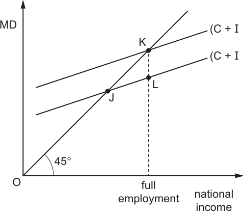
What does the distance KL represent?
Options
A a deflationary gap
B a trade deficit
C an inflationary gap
D an employment gap
Working
The diagram is a Keynesian cross model. The 45-degree line shows all points where aggregate expenditure (MD) equals national income, i.e., equilibrium. The current aggregate expenditure line (C + I + G + X - M)1 intersects the 45-degree line at J, so equilibrium national income is at J, which is below the full employment level of national income (marked by the vertical dashed line). A deflationary gap exists when equilibrium national income is less than full employment national income, representing the shortfall in aggregate expenditure needed to reach full employment. The distance KL is the gap between current aggregate expenditure at full employment income (point L) and the aggregate expenditure required for full employment equilibrium (point K), which is the deflationary gap. A trade deficit measures when imports exceed exports, which is not shown here. An inflationary gap occurs when equilibrium income is above full employment, which is not the case. There is no standard "employment gap" in this context.
Answer
A
A
Background Concept
The Keynesian cross diagram is a core model for national income determination. The vertical axis measures aggregate expenditure (also called aggregate demand, AD, labelled MD in this diagram), which is the total planned spending in the economy: consumption (C) + investment (I) + government spending (G) + exports (X) - imports (M). The horizontal axis measures national income (Y), which equals total output in the economy.
The 45-degree line from the origin plots all points where aggregate expenditure equals national income (Y = AD). This is the equilibrium condition: at any point on this line, total spending equals total output, so firms have no unplanned inventory changes and have no incentive to increase or decrease production. The intersection of an aggregate expenditure line and the 45-degree line is the equilibrium level of national income.
Full employment national income (also called potential output) is the level of national income at which all available labour and capital resources are fully utilised, with no cyclical unemployment. It is represented by a vertical line on the Keynesian cross, as it is independent of the level of aggregate expenditure.
A deflationary gap (or recessionary gap) occurs when the equilibrium level of national income is below the full employment level. This means there is insufficient aggregate demand to buy all the output the economy can produce at full employment, leading to unused capacity and cyclical unemployment. The size of the deflationary gap is the difference between full employment income and equilibrium income, and it represents the amount by which aggregate expenditure must increase to close the gap and reach full employment.
An inflationary gap is the opposite scenario: equilibrium national income is above the full employment level, meaning aggregate demand is too high, leading to demand-pull inflation as firms compete for scarce resources.
Understanding the Question
The question provides a Keynesian cross diagram with two aggregate expenditure lines, and states the economy is in equilibrium at point J (on the lower aggregate expenditure line and the 45-degree line). A vertical dashed line marks the full employment level of national income, which is to the right of J, meaning equilibrium income is below full employment. The question asks what the distance KL represents, where K is on the higher aggregate expenditure line at the full employment income level, and L is on the lower aggregate expenditure line at the same full employment income level.
The question tests recognition of national income gap concepts applied to a standard diagram. We need to match the diagram's configuration to the correct gap type, eliminating the three incorrect options.
Approach
First, eliminate clearly incorrect options:
- Option B (trade deficit): A trade deficit is a balance of payments concept where import value exceeds export value. While net exports (X-M) are a component of aggregate expenditure, KL does not measure the difference between exports and imports, so this is irrelevant.
- Option D (employment gap): This is not a standard term used in national income analysis to describe the difference between equilibrium and full employment income, so it can be discarded immediately.
Next, distinguish between the two remaining gap types:
- Deflationary gap: Equilibrium income < full employment income (the scenario in the diagram, as J is left of the full employment line).
- Inflationary gap: Equilibrium income > full employment income (not the case here, as J is left of the full employment line).
This leaves Option A as the only plausible answer. We can confirm by linking KL to the definition of a deflationary gap.
Step-by-Step Reasoning
- Interpret the diagram's components: The 45-degree line is the equilibrium line, where aggregate expenditure (AD) equals national income. The lower aggregate expenditure line (C + I + G + X - M)1 is the current level of total planned spending in the economy. Its intersection with the 45-degree line at J is the current equilibrium national income, which is lower than the full employment level (the x-coordinate of the vertical dashed line).
- Define the deflationary gap: A deflationary gap is the shortfall of equilibrium national income relative to the full employment level. It arises because current aggregate demand is too low to purchase all the output the economy can produce at full capacity. To close the gap, aggregate expenditure must increase, shifting the AE curve rightward until it intersects the 45-degree line at the full employment income level.
- Interpret points K and L: The vertical dashed line is at the full employment income level. Point L is the level of current aggregate expenditure (from the lower AE line) at this full employment income level. Point K is on the higher aggregate expenditure line at the same full employment income level, and lies on the 45-degree line, meaning this is the level of aggregate expenditure required for the economy to be in equilibrium at full employment.
- Link KL to the deflationary gap: The vertical distance KL is the difference between the required aggregate expenditure for full employment (point K) and the current aggregate expenditure at full employment income (point L). This difference is exactly the deflationary gap: it measures how much aggregate expenditure is currently falling short of the level needed to achieve full employment equilibrium. While the deflationary gap is often expressed as the horizontal difference between equilibrium income and full employment income, the vertical distance KL is an equivalent measure of the spending shortfall causing the gap.
- Confirm elimination of other options: As noted earlier, a trade deficit (B) is unrelated to the gap between equilibrium and full employment income. An inflationary gap (C) would require equilibrium income to be above full employment, which is not the case here. There is no standard macroeconomic concept of an "employment gap" (D) in this context.
Key Takeaways
- The Keynesian cross diagram identifies equilibrium national income at the intersection of the aggregate expenditure line and the 45-degree line.
- A deflationary gap exists when equilibrium income is below full employment income, indicating insufficient aggregate demand.
- An inflationary gap is the opposite, with equilibrium income above full employment, indicating excessive aggregate demand.
- Always check the position of the equilibrium point relative to the full employment line to identify the type of gap.
Common Mistakes
- Mixing up deflationary and inflationary gaps: Students often confuse which gap corresponds to equilibrium below vs above full employment. A simple mnemonic is: deflationary = below full employment (associated with recession, unused capacity), inflationary = above full employment (associated with overheating, demand-pull inflation).
- Misinterpreting the 45-degree line as the full employment line: The 45-degree line is the set of all equilibrium points, while full employment is a separate vertical line showing potential output. Confusing these leads to incorrectly identifying the gap type.
- Linking the gap to trade: Since aggregate expenditure includes net exports, students may incorrectly assume the gap relates to a trade deficit, but the gap here is between equilibrium and full employment income, not between export and import values.
- Selecting the non-standard "employment gap" option: This term is not used in standard Cambridge A-Level Economics to describe this scenario, so it can be eliminated immediately.
Things to Be Careful About
- Always verify the relative position of the equilibrium point and the full employment line: if equilibrium is to the left of full employment, it is a deflationary gap; if to the right, inflationary.
- The distance KL represents the vertical spending shortfall at full employment income, which is equivalent to the horizontal deflationary gap (adjusted for the marginal propensity to consume). In the context of this question, it is explicitly identified as the deflationary gap.
- Remember that the aggregate expenditure line includes all components of AD (C+I+G+X-M), so changes to any of these components shift the line and change the size of the deflationary or inflationary gap.
A country experiences an increase in unemployment due to deficiency of aggregate demand.
What will be the effect of this on tax revenue and government expenditure, assuming that tax rates and rates of unemployment benefit remain unchanged?
Options
| tax revenue | government expenditure | |
|---|---|---|
| A | decrease | increase |
| B | decrease | no change |
| C | increase | decrease |
| D | no change | increase |
Answer
A rise in unemployment caused by a deficiency of aggregate demand reduces incomes and spending. With unchanged tax rates, income tax and consumption tax revenues fall, so tax revenue decreases. At the same time, more people qualify for unemployment benefits, so government expenditure on benefits increases. The correct option is A.
A
Background Concept
This question tests the concept of automatic stabilisers in fiscal policy. Automatic stabilisers are features of the tax and benefit system that automatically dampen fluctuations in aggregate demand without discretionary government action. When the economy slows and unemployment rises, tax revenues fall and welfare spending rises, which injects net spending into the economy and cushions the downturn. The opposite happens in a boom. The two key automatic stabilisers here are:
- Progressive income tax and consumption taxes (VAT/sales tax): These are proportional to income and spending. When incomes fall, tax payments fall automatically.
- Unemployment benefits (and other means-tested welfare payments): These rise automatically as more people become eligible.
Understanding the Question
The question presents a scenario: a country experiences a rise in unemployment caused by a deficiency of aggregate demand (i.e., a demand-deficient or cyclical unemployment, not structural or frictional). It asks what happens to tax revenue and government expenditure, assuming tax rates and the rate of unemployment benefit are unchanged. The answer requires tracing the direct, automatic effects — not any discretionary policy change.
Approach
- Identify the immediate consequence of higher unemployment: lower total household income and lower consumer spending.
- Trace the effect on tax revenue: with unchanged tax rates, lower incomes and spending mean lower income tax and VAT receipts.
- Trace the effect on government expenditure: more unemployed people means more claimants for unemployment benefits, so government spending on benefits rises.
- Match this pair (tax revenue falls, government spending rises) to the options.
Step-by-Step Reasoning
- Step 1: Unemployment rises due to deficient AD. Firms produce less, so they lay off workers. National income (GDP) falls.
- Step 2: Effect on tax revenue. Most tax revenue comes from income tax (on wages and profits) and consumption taxes (VAT, sales tax). With fewer people employed and lower total wages, income tax receipts fall. With lower consumer spending, VAT receipts also fall. Since tax rates are unchanged, the fall in the tax base (income and spending) directly reduces revenue. So tax revenue decreases.
- Step 3: Effect on government expenditure. The government pays unemployment benefits to those who lose their jobs. With more unemployed people, the number of claimants rises. The benefit rate per person is unchanged, so total spending on benefits increases. So government expenditure increases.
- Step 4: Match to options. The pair is: tax revenue decreases, government expenditure increases. This corresponds to option A.
Key Takeaways
- Automatic stabilisers mean that during a recession, the government budget automatically moves towards a deficit (lower revenue, higher spending), which helps support aggregate demand.
- The question tests the ability to distinguish automatic effects from discretionary policy changes.
- Always trace the causal chain: change in economic activity -> change in tax base/benefit eligibility -> change in revenue/spending.
Common Mistakes
- Confusing automatic stabilisers with discretionary policy: Some students might think the government actively cuts taxes or raises spending, but the question explicitly says tax rates and benefit rates are unchanged.
- Thinking government expenditure is unchanged: A common error is to assume that because benefit rates are fixed, spending stays the same — but the number of claimants rises, so total spending rises.
- Reversing the direction: Some might think tax revenue rises because the government needs more money to pay benefits, but revenue depends on the tax base, not on spending needs.
Things to Be Careful About
- The question specifies "deficiency of aggregate demand" — this is demand-deficient unemployment, not structural or frictional. The mechanism is the same for any rise in unemployment that reduces incomes, but the cause matters for policy implications.
- The assumption of unchanged tax and benefit rates is crucial — without it, the answer could be different.
- Note that the government expenditure increase here is on transfer payments (benefits), not on goods and services. Transfer payments are counted as government expenditure in national accounts but do not directly add to GDP (they are transfers, not purchases).
A government is successful in raising the rate of economic growth.
As a result, which other macro-economic aim would it most likely have achieved in the short run?
Options
A balance of payments surplus
B higher employment
C lower inflation
D stronger exchange rate
Reasoning
In the short run, a government that successfully raises the rate of economic growth is likely to see higher output. To produce more goods and services, firms typically employ more workers, so unemployment falls and employment rises. This is the most direct short-run effect among the options. A balance of payments surplus is unlikely because higher national income tends to increase imports, worsening the current account. Lower inflation is not expected, as rising aggregate demand often fuels demand-pull inflation. A stronger exchange rate is not a guaranteed short-run outcome; it depends on interest rate responses and capital flows. Therefore, the macro-economic aim most likely to be achieved is higher employment.
Answer
B
B
Background Concept
In macroeconomics, governments pursue several objectives simultaneously: low inflation, low unemployment, sustainable economic growth, a stable balance of payments, and a stable exchange rate. In the short run, these objectives are not always compatible. The traditional Phillips curve illustrates a short-run trade-off between inflation and unemployment: when aggregate demand grows faster, output rises, unemployment falls, but inflation tends to increase. Economic growth (usually measured as the percentage increase in real GDP) is positively correlated with employment in the short run, because higher output requires more labour input — especially when there is spare capacity. This relationship is sometimes known as Okun’s law. However, the same growth may put upward pressure on the price level and can worsen the current account if the extra demand 'leaks' into imports.
Understanding the Question
The question asks: 'A government is successful in raising the rate of economic growth. As a result, which other macro-economic aim would it most likely have achieved in the short run?' Four options are given: balance of payments surplus, higher employment, lower inflation, and a stronger exchange rate. The phrase 'in the short run' is crucial — it directs us to consider immediate cyclical effects rather than long-run structural outcomes. We need to identify which of the four objectives is typically enhanced when growth accelerates, based on standard macroeconomic theory.
Approach
Evaluate each option against the likely short-run consequences of faster economic growth:
- Balance of payments surplus: Growth increases national income, which raises spending on imports. Unless exports rise at the same rate (unlikely in the short run), the current account worsens. So a surplus is improbable.
- Higher employment: As output expands, firms demand more labour. If the economy is operating below full employment, growth will reduce unemployment and raise employment. This is a well-established positive short-run relationship.
- Lower inflation: Faster growth, especially if demand-driven, tends to increase the general price level (demand-pull inflation). The Phillips curve suggests a negative short-run relationship between unemployment and inflation. Therefore, lower inflation is unlikely.
- Stronger exchange rate: The effect is ambiguous. Growth may attract foreign capital (if accompanied by higher interest rates) and appreciate the currency, but it could also increase imports and weaken the currency. Direct and immediate strengthening is not a predictable short-run outcome.
Thus, the most plausible and direct positive short-run effect is higher employment.
Step-by-Step Reasoning
- Start with the fact: The government has successfully raised the rate of economic growth (faster increase in real GDP).
- Identify the short-run mechanism: In the short run, with capital stock fixed, higher output requires more variable inputs, especially labour. Firms hire additional workers to meet the increased demand for goods and services. This reduces unemployment and increases employment.
- Check each option in turn:
- Option A (balance of payments surplus): Higher GDP raises disposable income, which typically increases import spending. Unless the growth is export-led (e.g., a boom in export industries), the current account moves towards deficit. A surplus is the opposite and therefore not likely.
- Option B (higher employment): As explained, this is directly linked. Growth in output generally pulls more people into work, especially if the economy was below full capacity. This is the standard result.
- Option C (lower inflation): According to the short-run Phillips curve, reduced unemployment (from faster growth) is associated with higher inflation, not lower. Demand-pull inflation tends to rise when AD grows faster than AS. So lower inflation is not expected.
- Option D (stronger exchange rate): The exchange rate is influenced by many factors: interest rates, capital flows, expectations, and the trade balance. Faster growth could theoretically attract foreign investment (if interest rates rise), leading to appreciation. However, stronger growth also raises imports, which could weaken the currency. The net effect is uncertain and not reliably positive in the short run. The question asks for 'most likely', making this option weaker than the clear employment link.
- Conclude: The only option with a clear, predictable, and positive short-run relationship to economic growth is higher employment (Option B).
Key Takeaways
- Economic growth and employment are positively correlated in the short run (Okun’s law).
- Growth often comes at the cost of higher inflation and a worsening current account.
- The exchange rate effect of growth is ambiguous and not a direct short-run priority.
- When answering multiple-choice questions on macro objectives, distinguish short-run from long-run effects and recall the trade-offs from the Phillips curve and other macro models.
Common Mistakes
- Assuming growth always reduces inflation: This is incorrect; demand-pull inflation usually accompanies faster growth unless the growth is purely supply-side driven in the long run.
- Thinking growth automatically strengthens the exchange rate: The exchange rate depends on interest rates and capital flows, not just output growth.
- Choosing the balance of payments surplus: Many students associate growth with export success, but in the short run, imports typically rise faster.
- Ignoring the 'short run' qualifier: Without it, supply-side growth could have different effects (e.g., lower inflation, stronger currency).
Things to Be Careful About
- Always read the question's time frame ('short run' vs 'long run') — it changes the expected answer.
- Remember that macro objectives often conflict in the short run: growth helps employment but worsens inflation and the current account.
- When eliminating options, use economic reasoning rather than intuition. For example, a balance of payments surplus is generally a sign of weak growth, not strong growth.
- The word 'most likely' allows for some uncertainty, but the employment link is the most direct and well-supported by theory.
Which argument for lowering income tax rates is always valid?
Options
A It boosts economic activity.
B It promotes the incentive to work.
C It reduces the budget deficit.
D It reduces the incentive to evade taxes.
Reasoning
The question asks which argument for lowering income tax rates is always valid. Each option must be tested against this absolute criterion.
A – Lower tax rates may boost economic activity if they increase disposable income and spending, but if the economy is already at full capacity, the effect may be inflationary rather than a real boost. Not always valid.
B – Lower tax rates can increase the incentive to work by raising the post-tax wage, but for workers who are already earning enough to meet their target income, a lower tax rate may reduce their need to work additional hours (the income effect may outweigh the substitution effect). Not always valid.
C – Lower tax rates reduce government revenue per unit of tax base, so unless the tax base expands sufficiently (the Laffer curve effect), the budget deficit will increase. The Laffer effect is not guaranteed. Not always valid.
D – Lower tax rates reduce the financial gain from evading taxes, because the difference between the legal tax paid and the illegal avoidance is smaller. This reduces the incentive to evade taxes. This is always true: a lower tax rate always reduces the marginal benefit of evasion, regardless of other conditions.
Answer
D
D
Background Concept
This question tests the ability to evaluate economic arguments against an absolute standard — the word 'always'. In economics, very few relationships are invariant across all circumstances. The Laffer curve is relevant: it shows that tax revenue may rise or fall when tax rates change, depending on the elasticity of the tax base. The incentive to work is affected by both substitution and income effects. The budget deficit depends on the balance between tax revenue and government spending. Tax evasion is a rational choice based on comparing the expected benefit (tax saved) with the expected cost (penalty times probability of detection).
Understanding the Question
The question presents four common arguments for lowering income tax rates and asks which one is 'always valid'. This is a critical thinking question: three of the statements are contingent on specific conditions and therefore not always true. Only one is logically necessary regardless of circumstances. The candidate must identify the one that holds under all possible scenarios.
Approach
Test each option against the 'always' criterion. For each, ask: 'Is there any plausible scenario in which this statement would be false?' If yes, eliminate it. The correct answer is the one that survives this test.
Step-by-Step Reasoning
Option A: 'It boosts economic activity.'
- Lower tax rates increase disposable income, which can raise consumption and aggregate demand. This could boost economic activity.
- However, if the economy is at full employment, the increase in demand may simply cause inflation without raising real output. Also, if the tax cut is financed by borrowing, higher interest rates could crowd out private investment, reducing economic activity. So the statement is not always true.
Option B: 'It promotes the incentive to work.'
- A lower tax rate increases the net wage, making work more attractive relative to leisure (substitution effect). This tends to increase labour supply.
- But for workers who have a target income, a higher net wage means they can reach that target with fewer hours, so they may choose to work less (income effect). The net effect on work incentive is ambiguous and depends on individual preferences. Not always true.
Option C: 'It reduces the budget deficit.'
- Lower tax rates reduce government revenue per unit of income. To reduce the deficit, the tax base must expand enough to offset the rate cut (the Laffer curve argument). This is not guaranteed; it depends on the elasticity of taxable income. In many cases, a tax cut increases the deficit. Not always true.
Option D: 'It reduces the incentive to evade taxes.'
- Tax evasion is a decision under uncertainty: the evader compares the benefit (tax saved) with the expected cost (penalty × probability of detection). A lower tax rate directly reduces the benefit of evasion — the amount saved per unit of concealed income is smaller. This reduces the incentive to evade, regardless of the penalty or detection probability. The statement is always true.
Key Takeaways
- The word 'always' in economics questions signals that only a logically necessary relationship qualifies. Most economic relationships are contingent on assumptions or conditions.
- Tax evasion is a rational choice model: lower tax rates reduce the marginal benefit of evasion, making it less attractive.
- The Laffer curve shows that tax cuts may increase or decrease revenue; they do not always reduce the deficit.
- The income and substitution effects on labour supply can work in opposite directions, so the net effect on work incentive is ambiguous.
Common Mistakes
- Choosing A or B because they seem intuitively plausible without considering counter-examples (full capacity, target income).
- Assuming that a tax cut always stimulates the economy, ignoring the possibility of crowding out or inflation.
- Confusing tax evasion (illegal) with tax avoidance (legal). The question is about evasion.
- Overlooking the 'always' qualifier and selecting a statement that is true in many cases but not all.
Things to Be Careful About
- Read the question carefully: 'always valid' is the key phrase. Do not settle for 'usually true'.
- For option C, remember that the Laffer curve is a theoretical possibility, not a guaranteed outcome. The question does not assume the economy is on the 'wrong side' of the curve.
- For option D, the logic is straightforward: a lower tax rate reduces the gain from evasion, so the incentive to evade falls. This is unconditional.
The table shows the percentage of labour force unemployed and the rate of inflation in a country over a five-year period.
| year | unemployment % | inflation % |
|---|---|---|
| 1 | 3.5 | 4.0 |
| 2 | 4.1 | 3.6 |
| 3 | 4.3 | 2.5 |
| 4 | 4.5 | 2.2 |
| 5 | 4.8 | 2.0 |
Which statement about the application of the Phillips curve theory to this country is most supported by the data?
Options
A The data are entirely consistent with the theory of the Phillips curve.
B The data prove conclusively that the Phillips curve theory does not operate.
C The data suggest that no conclusions can be reached about the validity of the Phillips curve theory.
D The data suggest that the theory of the Phillips curve is correct, though with time lags.
Reasoning
The traditional Phillips curve describes an inverse (trade-off) relationship between the rate of unemployment and the rate of inflation. The data show that as the unemployment rate rises from 3.5% to 4.8% over the five years, the inflation rate falls from 4.0% to 2.0%. This is exactly the pattern the Phillips curve predicts: lower inflation is associated with higher unemployment. The data are therefore entirely consistent with the theory.
Answer
A
A
Background Concept
The Phillips curve, originally observed by A.W. Phillips, shows an inverse (negative) relationship between the rate of unemployment and the rate of wage (and later price) inflation. The traditional (short-run) Phillips curve suggests that when unemployment is low, inflation tends to be high, and when unemployment is high, inflation tends to be low. This is because low unemployment puts upward pressure on wages as firms compete for scarce labour, which feeds through into higher prices. Conversely, high unemployment reduces wage pressure, leading to lower inflation. The curve is typically drawn with the unemployment rate on the horizontal axis and the inflation rate on the vertical axis, sloping downwards from left to right.
Understanding the Question
The question presents a table of data for a single country over five years, showing unemployment and inflation rates. It asks which statement about the application of Phillips curve theory to this country is most supported by the data. The four options range from full consistency (A), to conclusive disproof (B), to no conclusions possible (C), to consistency with time lags (D). The task is to see whether the observed pattern matches the predicted inverse relationship.
Approach
- Examine the data: note the direction of change in both variables over the five-year period.
- Recall the prediction of the traditional Phillips curve: an inverse relationship between unemployment and inflation.
- Compare the observed pattern to the prediction.
- Evaluate each option against the observed pattern.
Step-by-Step Reasoning
-
Read the data:
- Year 1: unemployment 3.5%, inflation 4.0%
- Year 2: unemployment 4.1%, inflation 3.6%
- Year 3: unemployment 4.3%, inflation 2.5%
- Year 4: unemployment 4.5%, inflation 2.2%
- Year 5: unemployment 4.8%, inflation 2.0%
-
Identify the trend:
- Unemployment rises steadily from 3.5% to 4.8% (an increase of 1.3 percentage points).
- Inflation falls steadily from 4.0% to 2.0% (a decrease of 2.0 percentage points).
-
Apply Phillips curve theory:
- The traditional Phillips curve predicts that as unemployment rises, inflation should fall. This is exactly what the data show. The inverse relationship is present and consistent across all five years.
-
Evaluate each option:
- Option A: "The data are entirely consistent with the theory of the Phillips curve." This is correct. The data show the predicted inverse relationship without any contradiction.
- Option B: "The data prove conclusively that the Phillips curve theory does not operate." This is false. The data support the theory, not disprove it.
- Option C: "The data suggest that no conclusions can be reached about the validity of the Phillips curve theory." This is false. The data clearly show the inverse relationship, so a conclusion can be reached.
- Option D: "The data suggest that the theory of the Phillips curve is correct, though with time lags." This is not the best answer. While time lags might exist in reality, the data show a contemporaneous inverse relationship (each year's unemployment and inflation move in opposite directions). There is no evidence of a lagged effect in the data, so this option introduces an unnecessary complication that is not supported.
-
Conclusion: Option A is the most supported statement.
Key Takeaways
- The traditional Phillips curve predicts an inverse relationship between unemployment and inflation.
- When interpreting data, look for the predicted pattern (one variable rising while the other falls).
- Be careful not to over-interpret: the data are consistent with the theory, but they do not "prove" it conclusively (other factors could also produce this pattern). Option A uses the word "consistent", which is appropriate.
- Avoid options that introduce unsupported claims (like time lags) or that overstate the conclusion (like "prove conclusively").
Common Mistakes
- Choosing Option D because students think Phillips curve effects always involve time lags. The data show a simultaneous inverse relationship, so there is no need to invoke lags.
- Choosing Option C because students think five data points are insufficient. While more data would be better, the data do show a clear pattern, so a conclusion can be reached.
- Misreading the data and thinking unemployment and inflation are moving in the same direction.
Things to Be Careful About
- Read the data carefully: note that unemployment rises and inflation falls.
- Understand the precise wording of each option. "Consistent with" is a weaker claim than "proves", and it is the correct level of certainty for this question.
- Do not confuse the traditional Phillips curve with the expectations-augmented Phillips curve, which introduces the concept of the natural rate of unemployment and suggests the trade-off may only exist in the short run. The question refers to the "Phillips curve theory" in general, and the data are consistent with the traditional version.
What indicates that a more equal distribution of income has been achieved?
Options
A a faster rate of economic growth
B a higher Human Development Index
C a lower Gini coefficient
D a lower tax /GDP ratio
Answer
The Gini coefficient is the standard measure of income inequality within a country. It ranges from 0 (perfect equality) to 1 (perfect inequality). A lower Gini coefficient therefore indicates a more equal distribution of income.
A is incorrect because a faster rate of economic growth does not guarantee a more equal distribution; growth can be concentrated among the wealthy.
B is incorrect because the Human Development Index (HDI) is a composite measure of life expectancy, education, and income per capita, not a direct measure of income distribution.
D is incorrect because a lower tax/GDP ratio indicates a smaller government sector relative to the economy, which does not directly imply a more equal income distribution.
C
Background Concept
The Gini coefficient is a statistical measure of income or wealth inequality within a nation or any other group of people. It is derived from the Lorenz curve, which plots the cumulative percentage of total income received against the cumulative percentage of the population (ordered from poorest to richest). The Gini coefficient is the ratio of the area between the line of perfect equality (the 45-degree line) and the Lorenz curve, divided by the total area under the line of perfect equality. The coefficient ranges from 0 (perfect equality, where everyone has the same income) to 1 (perfect inequality, where one person has all the income).
Understanding the Question
The question asks which of the four options is a direct indicator that a more equal distribution of income has been achieved. It tests the candidate's ability to distinguish between different macroeconomic indicators: economic growth (A), human development (B), income inequality (C), and the size of the government sector (D). The correct answer is the one that specifically measures how income is spread across the population.
Approach
To answer this question, recall the definition and purpose of each indicator:
- Economic growth measures the increase in a country's output (GDP). It does not inherently tell us anything about how that output is distributed.
- Human Development Index (HDI) is a composite statistic of life expectancy, education, and per capita income indicators. It measures average achievement, not distribution.
- Gini coefficient is the standard measure of income inequality. A lower value means the Lorenz curve is closer to the line of perfect equality.
- Tax/GDP ratio measures the total tax revenue collected by the government as a share of the economy. It is a measure of fiscal capacity or government size, not a direct measure of income distribution.
By process of elimination, the Gini coefficient is the only option that directly answers the question.
Step-by-Step Reasoning
- Option A (a faster rate of economic growth): Economic growth can occur alongside rising inequality (e.g., if growth is driven by capital-intensive industries that benefit the wealthy) or falling inequality (e.g., if growth is broad-based and raises the incomes of the poor). The Kuznets curve hypothesis even suggests that inequality first rises and then falls during the process of economic development. Therefore, a faster growth rate is not a reliable indicator of a more equal distribution.
- Option B (a higher Human Development Index): The HDI is a composite index that combines three dimensions: a long and healthy life (life expectancy), knowledge (education), and a decent standard of living (GNI per capita). While a higher HDI generally indicates better development outcomes, it does not measure how income is distributed within the country. A country could have a high HDI but high inequality (e.g., some oil-rich nations).
- Option C (a lower Gini coefficient): This is the correct answer. The Gini coefficient is specifically designed to measure income inequality. A lower coefficient means the country's income distribution is moving closer to perfect equality. This is the only option that is a direct measure of distribution.
- Option D (a lower tax/GDP ratio): The tax/GDP ratio indicates the proportion of a country's output that is collected by the government through taxes. A lower ratio could mean lower taxes, but this does not automatically imply a more equal distribution of income. The distributional impact of taxes depends on whether the tax system is progressive (taxing the rich more) or regressive (taxing the poor more). A lower tax/GDP ratio could even be associated with higher inequality if it results from cuts to progressive taxes.
Key Takeaways
- The Gini coefficient is the definitive statistical measure of income or wealth inequality.
- It is derived from the Lorenz curve.
- A lower Gini coefficient indicates a more equal distribution; a higher coefficient indicates a more unequal distribution.
- It is important to distinguish between indicators of growth (GDP), development (HDI), inequality (Gini), and government size (Tax/GDP).
Common Mistakes
- Confusing growth with equity: Students often assume that economic growth automatically leads to a more equal distribution of income. This is not necessarily true, as growth can be concentrated in specific sectors or among specific groups.
- Confusing development with distribution: The HDI is a measure of average achievement, not how that achievement is shared. A country can have a high HDI and high inequality.
- Misinterpreting the Gini coefficient: Forgetting the scale (0 = perfect equality, 1 = perfect inequality) and thinking a higher coefficient means more equality.
Things to Be Careful About
- Precise definitions: Know the exact definition and purpose of each economic indicator.
- Direct vs. indirect measures: The question asks for an indicator that indicates a more equal distribution. The Gini coefficient is a direct measure. The other options are indirect or unrelated.
- The Lorenz curve: Understanding the graphical representation of the Lorenz curve helps solidify the concept of the Gini coefficient.
In 2018, the United States (US) government introduced tariffs on a wide range of imports from China.
Which type of policy was the US government adopting?
Options
A expenditure-reducing
B expenditure-switching
C expansionary monetary
D contractionary monetary
Working
Tariffs are taxes on imported goods. They increase the price of imports relative to domestic goods, encouraging consumers to switch expenditure from imports to domestically produced goods. This is the essence of an expenditure-switching policy, which aims to correct a balance of payments deficit by redirecting spending.
Expenditure-reducing policies lower aggregate demand, contractionary monetary policy reduces the money supply, and expansionary monetary policy increases it. None of these involve trade barriers.
Answer
B
B
Background Concept
In macroeconomics, policies to correct a current account deficit fall into two categories: expenditure-reducing policies and expenditure-switching policies. Expenditure-reducing policies aim to lower aggregate demand (e.g., contractionary fiscal or monetary policy), which reduces the demand for imports because total spending falls. Expenditure-switching policies aim to change the relative prices of domestic and foreign goods so that consumers switch from imports to domestic products. Common tools include devaluation/depreciation of the currency, tariffs (import taxes), quotas, and export subsidies. Tariffs specifically raise the price of imported goods, making domestic goods relatively cheaper, thus encouraging domestic consumers to buy local products instead of imports.
Understanding the Question
The question presents a factual event: in 2018, the US imposed tariffs on Chinese imports. It asks which type of policy this represents: expenditure-reducing, expenditure-switching, expansionary monetary, or contractionary monetary. This is a classification question that tests understanding of the definitions of these policy categories.
Approach
Recognise that tariffs are a trade barrier that directly affect relative prices, not aggregate demand or the money supply. Therefore the answer must be expenditure-switching. Eliminate the other options by understanding what they entail: expenditure-reducing uses demand management to cut imports; monetary policies affect interest rates and the money supply, not trade barriers.
Step-by-Step Reasoning
-
Expenditure-reducing policy: This includes any policy that reduces total spending in the economy, such as higher taxes, lower government spending, or higher interest rates. The aim is to reduce imports because lower income reduces import demand. Tariffs do not reduce aggregate demand directly; they may even have a small inflationary effect. So A is incorrect.
-
Expenditure-switching policy: This changes the relative price of imports compared to domestic goods. A tariff adds a tax on imports, making them more expensive. Domestic goods become relatively cheaper, so consumers switch from imports to domestic goods. This exactly describes a tariff. So B is correct.
-
Expansionary monetary policy: This involves lowering interest rates or increasing the money supply to boost aggregate demand. It would likely increase imports, not reduce them. Tariffs are not a monetary tool. So C is incorrect.
-
Contractionary monetary policy: This involves raising interest rates or reducing the money supply to cool demand. While this could reduce imports by lowering income, it is not what tariffs do. Tariffs are a trade policy, not a monetary policy. So D is incorrect.
Thus the correct classification is expenditure-switching.
Key Takeaways
- Expenditure-switching policies change relative prices to redirect spending from foreign to domestic goods.
- Tariffs, quotas, and devaluation are key examples.
- Expenditure-reducing policies lower aggregate demand to cut imports.
- Monetary policies affect the money supply and interest rates; they are not trade policies.
Common Mistakes
- Confusing expenditure-reducing with expenditure-switching: both can reduce imports, but the mechanism is different. Expenditure-reducing cuts total spending; expenditure-switching redirects spending.
- Thinking tariffs are a form of monetary policy because they affect prices; but monetary policy refers to central bank actions on money and credit.
- Failing to recognise that the question is about classification, not evaluation of effectiveness.
Things to Be Careful About
- Definitions: expenditure-switching does not necessarily reduce the total value of imports; it reduces the volume/share of imports relative to domestic goods. Expenditure-reducing reduces the total.
- The question is specific to policy type, not the debate over whether the tariff was effective.
A US company receives a US$20 million dividend from shares that it owns in a Brazilian company.
How would this dividend be shown in the balance of payments of the United States?
Options
A a credit in the capital account
B a credit in the current account
C a debit in the capital account
D a debit in the current account
Working
Dividends from foreign shares are income from a foreign investment. In the balance of payments, income from foreign investments is recorded in the current account under 'primary income'. Since the US company receives the dividend, it is a receipt for the US, so it is a credit entry.
Therefore, the dividend is a credit in the current account.
Answer
B
B
Background Concept
The balance of payments is a record of all economic transactions between residents of one country and the rest of the world over a period. It has three main accounts:
- Current account: records trade in goods (visible trade), services (invisible trade), primary income (income from investments such as dividends, interest, and profits), and secondary income (transfers). A credit in the current account represents an inflow of funds (e.g. exports, income received from abroad). A debit represents an outflow (e.g. imports, income paid abroad).
- Capital account: records capital transfers (e.g. debt forgiveness) and acquisition/disposal of non-produced, non-financial assets (e.g. patents). It is relatively small for most economies.
- Financial account: records transactions in financial assets and liabilities, such as direct investment, portfolio investment, and reserve assets. This is where the purchase of shares in a Brazilian company by a US resident would appear as a financial outflow (debit), not the income from those shares.
Dividends are a return on equity investment. They represent a flow of income from the country where the investment is made to the country of the investor. Therefore, they belong in the current account as primary income.
Understanding the Question
The question describes a specific transaction: a US company receives a US$20 million dividend from shares it owns in a Brazilian company. The question asks how this dividend would be shown in the US balance of payments — specifically, which account and whether it is a credit or a debit. The options present a combination of 'credit/debit' and 'current account/capital account'. (Note: In the Cambridge 9708 syllabus, the capital account and financial account are separate, but here 'capital account' in the options likely refers to the broader capital and financial account as sometimes used loosely; however, the correct answer must differentiate based on the actual classification.) The transaction is an inflow of funds to the US: the dividend is received by the US company from abroad.
Approach
To answer, recall the standard classification of international transactions:
- Income flows from foreign investments (dividends, interest, profits) are part of primary income in the current account.
- An inflow of funds (receipt) is a credit; an outflow (payment) is a debit.
Since the US company is receiving the dividend, it is a credit to the US balance of payments. The incorrect options involve the capital account or a debit, which do not fit the nature of the transaction.
Step-by-Step Reasoning
-
Identify the nature of the transaction: The US company owns shares in a Brazilian company. The dividend is the return on that investment. It is not the purchase or sale of the shares themselves, which would be a financial account transaction. Instead, it is income earned from the investment.
-
Determine the correct account: According to the IMF's Balance of Payments Manual (and the Cambridge A-Level syllabus), investment income is recorded in the current account under 'primary income'. Therefore, the dividend belongs in the current account, not the capital account.
-
Determine the direction: The dividend is paid by the Brazilian company (resident of Brazil) to the US company (resident of the US). Money flows from Brazil to the US. For the US, this is a receipt, i.e., an inflow. In the balance of payments, inflows are recorded as credits (positive entries). So it is a credit.
-
Eliminate incorrect options:
- Option A: credit in the capital account — incorrect because capital account records capital transfers and non-produced assets, not income flows.
- Option C: debit in the capital account — incorrect for the same reason and because it is a receipt, not a payment.
- Option D: debit in the current account — incorrect because it is an inflow, so it must be a credit.
-
Therefore, the correct answer is B: a credit in the current account.
Key Takeaways
- Investment income (dividends, interest, profits) is recorded in the current account, not the financial account.
- Inflows are credits; outflows are debits.
- Distinguish between the flow of income from an investment (current account) and the flow of the investment principal (financial account).
Common Mistakes
- Confusing the financial account with the current account: many students think that because the US company owns shares (a financial asset), the dividend must be in the financial account. However, the financial account records the acquisition and disposal of assets, not the income generated by them.
- Misidentifying the sign: a receipt from abroad is a credit. Some students incorrectly think all foreign receipts are debits because they confuse 'credit' with 'positive' in a current account deficit context.
- Thinking that dividends are capital transfers: dividends are not transfers; they are a return on investment and are classified as income.
Things to Be Careful About
- In some older presentations (pre-IMF BPM6), the current account included only goods and services, and investment income was sometimes in the capital account. However, the Cambridge 9708 syllabus follows the standard modern classification where primary income is in the current account.
- The wording of the options uses 'capital account' which in the syllabus context usually means the capital account (transfers and non-produced assets) separate from the financial account. Do not confuse it with the broader 'capital and financial account' sometimes used in older textbooks.
- Always check the direction: who receives the payment? That determines credit/debit.
Conclusion
The correct answer is B: the dividend is a credit in the current account.
An increase or decrease in exchange rates can take place in both a floating and a fixed exchange rate system but different terminology is used for each system.
What is the correct terminology?
Options
| floating rate decreases | fixed rate increases | |
|---|---|---|
| A | depreciation | appreciation |
| B | depreciation | revaluation |
| C | devaluation | appreciation |
| D | devaluation | revaluation |
Reasoning
Under a floating exchange rate system, a decrease in the value of the currency is called depreciation; an increase is called appreciation. Under a fixed exchange rate system, a decrease is called devaluation; an increase is called revaluation. The question asks for a decrease in a floating rate (depreciation) and an increase in a fixed rate (revaluation), which matches option B.
Answer
B
B
Background Concept
Exchange rates can be determined in two broad systems: floating (market-determined) and fixed (government-determined). The terminology for a change in the value of a currency differs depending on the system. For a floating exchange rate, a fall in value is called depreciation, a rise is called appreciation. For a fixed exchange rate, a government-announced reduction in the value is called devaluation, an increase is called revaluation. This distinction is essential because the mechanism of change is different: under floating, it's a market movement; under fixed, it's a deliberate policy adjustment.
Understanding the Question
The question asks to match the correct terminology for two scenarios: when the exchange rate decreases under a floating system, and when the exchange rate increases under a fixed system. You are given a table with two columns: "floating rate decreases" and "fixed rate increases". The correct terms are depreciation (for floating decrease) and revaluation (for fixed increase). The distractors mix up the terms (e.g., using devaluation for floating, or appreciation for fixed).
Approach
Recall the definitions: floating: depreciation (down), appreciation (up). Fixed: devaluation (down), revaluation (up). Then apply to the two scenarios. Option B correctly pairs depreciation with floating decrease and revaluation with fixed increase.
Step-by-Step Reasoning
- Identify the exchange rate system for each column.
- "floating rate decreases" refers to a floating system.
- "fixed rate increases" refers to a fixed system.
- Recall the terminology:
- Floating: a decrease is depreciation.
- Floating: an increase is appreciation.
- Fixed: a decrease is devaluation.
- Fixed: an increase is revaluation.
- Match the first column: floating rate decreases -> depreciation.
Match the second column: fixed rate increases -> revaluation. - Option B: depreciation | revaluation (depreciation first, revaluation second) is correct.
Option A: appreciation for fixed increase is wrong.
Option C: devaluation for floating decrease is wrong.
Option D: devaluation for floating decrease is wrong; revaluation for fixed increase is correct but the first column is wrong.
Key Takeaways
- Always distinguish the system when using terms: floating uses depreciation/appreciation; fixed uses devaluation/revaluation.
- The same direction of change (increase or decrease) can have different names depending on the regime.
Common Mistakes
- Using "devaluation" for a floating rate decrease (common error).
- Using "appreciation" for a fixed rate increase (appreciation is a market movement, not a policy change).
- Confusing the two columns: the question clearly labels the system, so read carefully.
Things to Be Careful About
- The wording "an increase or decrease in exchange rates can take place in both a floating and a fixed exchange rate system" sets up the context: you must use the correct system-appropriate term.
- Note that the first column says "floating rate decreases" (not "floating rate increases"), and the second says "fixed rate increases" (not "fixed rate decreases"). Answer accordingly.
Company X is a multinational company that produces batteries for electric cars. It decides to invest in a new factory in country N.
Under which conditions is this investment most likely to improve the current account balance on the balance of payments in country N?
Options
| % of raw materials used to make batteries supplied by country N | income elasticity of demand for electric cars outside country N | |
|---|---|---|
| A | 10 | 0.5 |
| B | 10 | 1.5 |
| C | 90 | 0.5 |
| D | 90 | 1.5 |
The current account balance improves when exports increase relative to imports. The investment in a new factory will produce batteries for export, but it may also require imports of raw materials. The current account improves if the net export effect is positive. The conditions favouring improvement are: a high percentage of raw materials supplied by country N (90%) reduces imports, and a high income elasticity of demand for electric cars outside country N (1.5) means that as global income grows, demand for exports will increase more than proportionally. Therefore, option D is most likely to improve the current account balance.
Answer
D
D
Background Concept
The balance of payments consists of the current account (trade in goods and services, income, transfers) and the financial account (capital flows). Foreign direct investment (FDI) is a financial account inflow. However, the investment can affect the current account through its impact on production and trade. When a multinational builds a factory, it may import raw materials and machinery, and later export the finished goods. The net effect on the current account depends on the difference between the value of exports generated and the value of imports required. Income elasticity of demand measures how responsive demand for a good is to changes in income. A good with income elasticity >1 is a luxury; demand grows faster than income. For an export good, a high income elasticity means that as global incomes rise, export demand will increase strongly, boosting the current account.
Understanding the Question
The question asks: under which conditions (combination of local raw material sourcing and income elasticity of export demand) is FDI most likely to improve the current account? The table gives two levels for each: 10% or 90% of raw materials supplied locally, and income elasticity of 0.5 or 1.5. The correct answer is the combination that maximizes the net export surplus: low imports (high local sourcing) and high export responsiveness (high income elasticity). Option D provides both.
Approach
Compare the two variables independently. For imports: the higher the percentage of raw materials sourced locally, the lower the import bill, so less leakage from the current account. For exports: the higher the income elasticity of demand for the product, the more exports will grow as world income rises, improving the current account. The best combination is both high. Therefore, D is correct.
Step-by-Step Reasoning
- Option A: 10% local sourcing → 90% of raw materials imported, so large import bill. Income elasticity 0.5 → demand for exports is relatively inelastic to income; even if world income grows, export demand increases only modestly. Net effect on current account is likely negative or small.
- Option B: 10% local sourcing (high imports) but income elasticity 1.5 (high). Exports may grow strongly, but the import bill is also high. The net effect could be positive if export growth is strong enough, but the high import content reduces the improvement. Not the best.
- Option C: 90% local sourcing (low imports) but income elasticity 0.5 (low). Exports grow slowly, so the current account improvement is limited by weak export demand growth.
- Option D: 90% local sourcing (low imports) and income elasticity 1.5 (high). Imports are minimal, and exports grow strongly with world income. This combination is most likely to yield a net improvement in the current account. Therefore, D is correct.
Key Takeaways
- FDI can improve the current account if it leads to net exports.
- The import content of production is crucial: local sourcing reduces imports.
- The income elasticity of demand for exports determines how much exports grow as the world economy expands.
- When both conditions are favourable, the current account improvement is most likely.
Common Mistakes
- Focusing only on the export side without considering the import content.
- Assuming that any FDI improves the current account; in reality, if the factory imports a lot of inputs, the net effect could be negative.
- Misinterpreting income elasticity: a low elasticity does not necessarily mean export demand is low, but it means it grows slowly with income.
- Forgetting that the question is about the current account, not the financial account.
Things to Be Careful About
- The percentage of raw materials supplied by country N is the share of inputs sourced locally; the rest is imported.
- Income elasticity of demand: 1.5 means that a 1% increase in income leads to a 1.5% increase in demand; 0.5 means a 0.5% increase.
- The question asks "most likely to improve", so we are looking for the combination that gives the highest probability of improvement.
- The investment itself is a financial inflow, but that is not part of the current account.
The diagram shows two Lorenz curves.
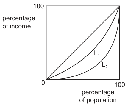
If the Lorenz curve shifts from L1 to L2, what is least likely to have caused this?
Options
A Capital gains tax has been reduced.
B Income tax has been made more progressive.
C Inheritance tax has been reduced.
D The tax-free allowance has been decreased for everyone.
Reasoning
The shift from L1 to L2 moves the Lorenz curve further from the line of perfect equality, indicating an increase in income inequality (a larger share of total income is held by a smaller share of the population).
- Option A: Reducing capital gains tax increases after-tax income for higher-income households (who own more assets) more than for low-income households, worsening inequality and causing the shift.
- Option B: A more progressive income tax takes a higher proportion of income from high earners, reducing disposable income inequality. This would move the Lorenz curve closer to the line of equality, so it is least likely to cause the L1 to L2 shift.
- Option C: Reducing inheritance tax benefits wealthier households (more likely to receive inheritances), increasing wealth-derived income and worsening inequality, causing the shift.
- Option D: Reducing the tax-free allowance increases the tax burden proportionally more for low-income households (who previously paid tax on a smaller share of their income) than for high-income households, worsening inequality and causing the shift.
Answer
B
B
Background Concept
Lorenz curves are a graphical tool used to measure the distribution of income (or wealth) across a population. The horizontal axis plots the cumulative percentage of the population (ordered from lowest to highest income), and the vertical axis plots the cumulative percentage of total income earned by that group. The 45-degree diagonal line of perfect equality represents a situation where each percentage of the population earns exactly that percentage of total income (for example, the bottom 50% of the population earns 50% of total income). A Lorenz curve that lies further below this line indicates greater income inequality, as a smaller share of the population holds a larger share of total income. The Gini coefficient, calculated as the area between the line of equality and the Lorenz curve divided by the total area under the line of equality, quantifies this inequality: a higher Gini coefficient means greater inequality.
Tax policies are a key tool for redistributing income:
- A progressive tax takes a larger proportion of income from high earners than low earners, reducing disposable income inequality.
- A regressive tax takes a larger proportion of income from low earners than high earners, worsening inequality.
- A proportional (flat) tax takes the same proportion of income from all earners, leaving the distribution of disposable income unchanged relative to pre-tax income.
Capital gains tax is levied on profits made from selling assets (for example, stocks, property), which are disproportionately owned by higher-income households. Inheritance tax is levied on the value of assets passed on to heirs after death, which also disproportionately benefits higher-income households who are more likely to inherit significant wealth. The tax-free allowance (also called the personal allowance) is the amount of income a household can earn before paying any income tax.
Understanding the Question
The question provides a diagram of two Lorenz curves, L1 and L2, where L2 is further from the line of perfect equality than L1. This means the shift from L1 to L2 represents an increase in income inequality: a smaller share of the population now holds a larger share of total income. The question asks which of the four listed policy changes is least likely to have caused this increase in inequality. This is an application question testing understanding of how fiscal policy tools affect income distribution, and how to interpret Lorenz curve shifts. The key is to identify the policy that would either reduce inequality or have no effect on it, rather than increasing it.
Approach
First, confirm the meaning of the Lorenz curve shift: L1 to L2 = increased income inequality. Then, for each option, analyse the likely effect of the policy change on the distribution of disposable income, focusing on which income groups are most affected by the tax change. The policy that reduces inequality (or has no effect) is the least likely cause of the shift, so that is the correct answer.
Step-by-Step Reasoning
- Interpret the Lorenz curve shift: The line of perfect equality is the 45-degree line where cumulative percentage of the population equals cumulative percentage of income. L2 lies further below this line than L1, meaning inequality has risen. We need to find the policy least likely to cause this rise.
- Evaluate Option A (Capital gains tax reduced): Capital gains are earned primarily by higher-income households, as they own far more financial and property assets than low-income households. Reducing the tax rate on capital gains increases the after-tax income of high earners by more than it increases the after-tax income of low earners (who rarely earn capital gains). This widens the gap between high and low disposable incomes, increasing inequality. This would cause the L1 to L2 shift, so it is not the correct answer.
- Evaluate Option B (Income tax made more progressive): A progressive income tax system charges higher tax rates on higher income brackets. Making the tax more progressive increases the average tax rate for high earners and reduces it (or leaves it unchanged) for low earners. This reduces the disposable income of high earners proportionally more than low earners, narrowing the income gap and reducing inequality. A reduction in inequality would shift the Lorenz curve closer to the line of equality (from L2 back to L1), so this policy is least likely to cause the L1 to L2 shift. This is the correct answer.
- Evaluate Option C (Inheritance tax reduced): Inheritance tax is paid on the value of assets passed on to heirs after death. Higher-income households are far more likely to receive large inheritances (of property, investments, etc.) than low-income households. Reducing inheritance tax increases the net wealth (and thus future income) of high-income households more than low-income households, widening the wealth and income gap over time. This increases inequality, so it would cause the L1 to L2 shift, so it is not the correct answer.
- Evaluate Option D (Tax-free allowance decreased for everyone): The tax-free allowance is the amount of income a household pays no tax on. Reducing this allowance means all households pay tax on a larger share of their income. However, low-income households previously paid tax on a smaller share of their income (since their total income was closer to the old allowance level) than high-income households (who already paid tax on most of their income). For example, if the allowance falls from £12,000 to £10,000: a household earning £15,000 now pays tax on £5,000 instead of £3,000, an extra tax burden equal to 13.3% of their total income; a household earning £100,000 now pays tax on £90,000 instead of £88,000, an extra burden equal to 0.4% of their total income. This regressive effect increases disposable income inequality, so it would cause the L1 to L2 shift, so it is not the correct answer.
- Conclusion: Only Option B would reduce inequality, so it is the least likely cause of the shift from L1 to L2.
Key Takeaways
- A Lorenz curve further from the line of equality indicates greater income inequality.
- Progressive tax policies reduce income inequality, while regressive tax policies increase it.
- Tax changes that disproportionately benefit high-income households (for example, cutting taxes on capital or inheritance) worsen inequality, while changes that increase the tax burden on high earners reduce inequality.
- Changes to the tax-free allowance are regressive if applied uniformly, as they take a larger share of income from low earners.
Common Mistakes
- Confusing Lorenz curve direction: Some students think a curve further from the line of equality means less inequality, but it is the opposite: greater distance from the line means a more unequal distribution of income.
- Misidentifying progressive tax effects: Some students assume any tax cut reduces inequality, but cutting taxes that are paid mostly by the rich (like capital gains tax) increases inequality, while making income tax more progressive reduces it.
- Ignoring who pays each tax: Students may assume all taxes affect everyone equally, but capital gains, inheritance and higher-rate income tax are paid almost exclusively by the wealthy, so changes to these taxes have disproportionate effects on high-income households.
- Misanalysing the tax-free allowance: Students may think cutting the allowance affects everyone equally, but it is regressive because low earners were previously exempt from tax on a larger share of their income, so the change hits their disposable income harder.
- Misreading the question: Some students may look for the policy that causes the shift, rather than the one that is least likely to cause it, leading them to pick the wrong option.
Things to Be Careful About
- Always link the position of the Lorenz curve to the level of inequality: further from the line of perfect equality = greater inequality, closer = less inequality.
- When evaluating tax policies, think about which income groups are most affected by the tax change, not just whether the tax is increased or decreased.
- For "least likely" questions, actively look for the option that would have the opposite effect (reduce inequality) rather than just a smaller increase in inequality.
- Remember that Lorenz curves measure the distribution of disposable income, so focus on after-tax effects of policy changes, not pre-tax income.
What is a likely result of globalisation?
Options
A Absolute advantage replaces comparative advantage as the basis for trade.
B Firms’ supply chains are shortened.
C Trade is less likely to suffer from international economic shocks.
D There are higher standards of living.
Answer
Globalisation involves the increasing integration of economies through trade, investment, and the movement of labour and capital. A likely result is that countries experience higher standards of living as they benefit from specialisation, economies of scale, and access to a wider variety of goods and services. Option D is correct.
Option A is incorrect because comparative advantage, not absolute advantage, remains the basis for trade. Option B is incorrect because globalisation typically lengthens supply chains as firms source inputs from around the world. Option C is incorrect because increased interdependence makes trade more vulnerable to international economic shocks.
D
Background Concept
Globalisation refers to the growing interdependence of economies worldwide through cross-border flows of goods, services, capital, labour, technology, and information. It is driven by trade liberalisation, advances in transport and communication, and the activities of multinational corporations. The key economic consequences include increased trade, greater specialisation according to comparative advantage, economies of scale, technology transfer, and higher living standards for many countries. However, it also brings risks such as greater vulnerability to global shocks, increased inequality, and environmental concerns.
Understanding the Question
This is a multiple-choice question asking for a likely result of globalisation. The candidate must identify which of the four options is a well-established consequence. The distractors present common misconceptions: that globalisation changes the basis of trade, shortens supply chains, or reduces vulnerability to shocks. The correct answer is the one that aligns with the standard economic analysis of globalisation's benefits.
Approach
Evaluate each option against the definition and known effects of globalisation. Eliminate those that contradict established theory or empirical evidence. The correct answer should be a widely accepted outcome.
Step-by-Step Reasoning
- Option A: Absolute advantage replaces comparative advantage as the basis for trade. This is false. Comparative advantage (the ability to produce a good at a lower opportunity cost) remains the fundamental reason for trade, even if a country has an absolute advantage in everything. Globalisation does not change this principle.
- Option B: Firms’ supply chains are shortened. This is the opposite of what happens. Globalisation encourages firms to source inputs from the cheapest locations worldwide, often lengthening and fragmenting supply chains across many countries.
- Option C: Trade is less likely to suffer from international economic shocks. This is incorrect. Greater interdependence means that a recession or financial crisis in one major economy can quickly spread to others through trade and financial links. Globalisation increases, not decreases, vulnerability to shocks.
- Option D: There are higher standards of living. This is correct. Globalisation allows countries to specialise according to comparative advantage, achieve economies of scale, access new technologies, and benefit from increased competition and consumer choice. These factors tend to raise productivity and real incomes, leading to higher living standards over time.
Key Takeaways
- Globalisation increases economic integration and interdependence.
- It is associated with higher living standards through specialisation, economies of scale, and technology transfer.
- It does not change the basis of trade (comparative advantage remains key).
- It typically lengthens supply chains and increases vulnerability to international shocks.
Common Mistakes
- Confusing absolute advantage with comparative advantage. The basis for trade is comparative advantage, not absolute advantage.
- Assuming that globalisation shortens supply chains. In reality, it often lengthens them as firms seek the cheapest inputs globally.
- Thinking that interdependence reduces risk. In fact, it can amplify the transmission of economic shocks.
Things to Be Careful About
- Read each option carefully and consider whether it aligns with the standard economic analysis of globalisation.
- Avoid choosing an option that sounds positive but is not a direct consequence of globalisation (e.g., higher living standards is a direct consequence, not just a general benefit).
Your score so far
Answer a question to start scoring
Your marks add up here as you work through the paper.