Economics 9708/31 — October/November 2024
Cambridge A-Level · A Level Multiple Choice · answer key with instant marking and worked solutions
Topics Growth and Survival of Firms · Employment and Unemployment · Costs of Production · Government Policies to Correct Market Failure · Demand for and Supply of Labour · Macroeconomic Objectives and Policy Conflicts · +14 more
Tap an option under each question to check it — your score builds as you go.
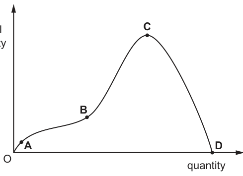
The diagram shows a total utility curve for a consumer.
At which point does marginal utility equal zero?
Options
A point A on Fig. 1.1
B point B on Fig. 1.1
C point C on Fig. 1.1
D point D on Fig. 1.1
Marginal utility (MU) is the change in total utility from consuming one more unit, represented by the slope of the total utility curve. MU equals zero when total utility is at its maximum. In Fig. 1.1, point C is the peak of the total utility curve, so marginal utility equals zero at point C.
Answer
C
C
Background Concept
Total utility (TU) is the total satisfaction a consumer derives from consuming a given quantity of a good or service. Marginal utility (MU) is the change in total utility from consuming one additional unit. Mathematically, MU corresponds to the slope (gradient) of the TU curve.
As consumption increases, total utility typically rises at a decreasing rate due to the law of diminishing marginal utility. Eventually, total utility reaches a maximum point. At this peak, the slope of the TU curve is zero, meaning marginal utility has fallen to zero. Beyond this point, if consumption continues, total utility falls and marginal utility becomes negative.
Understanding the Question
The question presents a diagram of a total utility curve (Fig. 1.1) with quantity on the horizontal axis and total utility on the vertical axis. The curve rises from the origin through points A and B, reaches a maximum at point C, and then falls to point D on the horizontal axis. The question asks at which point marginal utility equals zero.
This is a 1-mark multiple-choice question testing the fundamental relationship between total utility and marginal utility. The task is to identify the specific point on the diagram where MU = 0.
Approach
The key relationship to apply is: marginal utility equals zero at the maximum point of the total utility curve. This is because MU is the slope of the TU curve. When the curve is rising, the slope is positive (MU > 0). When the curve is at its peak, the slope is zero (MU = 0). When the curve is falling, the slope is negative (MU < 0).
Therefore, the task is simply to identify the peak of the curve in Fig. 1.1.
Step-by-Step Reasoning
- Analyse point A: The curve is rising from O to A. The slope is positive, so marginal utility is positive (MU > 0).
- Analyse point B: The curve is still rising, though at a slower rate. The slope remains positive, so MU > 0.
- Analyse point C: This is the highest point on the curve — the peak. At the exact peak of a total utility curve, the slope is zero. Therefore, marginal utility equals zero at point C. This is the point of satiety, where the consumer has gained maximum possible satisfaction from the good.
- Analyse point D: The curve has fallen to the horizontal axis, meaning total utility is zero. However, the curve is still falling as it approaches the axis, so the slope is negative. This means marginal utility is negative (MU < 0). Consuming beyond point C actually reduces total utility.
Thus, the correct answer is point C.
Key Takeaways
- Marginal utility is the slope (gradient) of the total utility curve, not the value of total utility itself.
- MU = 0 at the maximum point of the TU curve.
- MU > 0 when TU is rising.
- MU < 0 when TU is falling.
- The point where TU = 0 (point D) is not the same as the point where MU = 0.
Common Mistakes
- Confusing TU with MU: Some students select point D because total utility is zero there, but the question asks where marginal utility equals zero, not total utility.
- Misidentifying the peak: Failing to recognise that point C is the maximum point of the curve.
- Confusing slope with level: Not understanding that MU relates to the rate of change (slope) of TU, not the absolute level of TU.
Things to Be Careful About
- Always check whether the question asks about total utility or marginal utility. They move together but are not the same.
- On a TU curve, the peak is where the tangent is horizontal (slope = 0), which corresponds to MU = 0.
- If the curve continues to fall below the axis, MU remains negative; it does not become zero again simply because TU hits zero.
What is a characteristic of an indifference curve?
Options
A It will remain concave to the origin of the diagram.
B It will remain convex to the origin of the diagram.
C It can intersect other indifference curves at any point.
D The lower the indifference curve, the greater the satisfaction attainable.
Reasoning
An indifference curve shows all combinations of two goods that give a consumer the same level of utility. A standard property is that indifference curves are convex to the origin, reflecting a diminishing marginal rate of substitution. They are not concave (A), they cannot intersect (C), and higher curves represent greater satisfaction, not lower ones (D).
Answer
B
B
Background Concept
An indifference curve is a fundamental tool in consumer theory. It maps all bundles of two goods (say, good X and good Y) that yield the same total utility to the consumer. The consumer is indifferent between any two points on the same curve. The shape and properties of these curves are derived from assumptions about consumer preferences: completeness, transitivity, non-satiation (more is preferred to less), and a diminishing marginal rate of substitution (MRS). The MRS is the rate at which a consumer is willing to give up units of Y to gain one more unit of X while keeping utility constant. Diminishing MRS means that as the consumer has more X, they are willing to give up less and less Y for an additional unit of X, which gives the curve its characteristic convex shape.
Understanding the Question
This is a multiple-choice question asking for a correct characteristic of an indifference curve. Four statements are given, and only one is true. The question tests knowledge of the standard properties of indifference curves as taught in the A-Level syllabus. The correct answer is the one that is always true for a well-behaved indifference curve.
Approach
Recall the four key properties of indifference curves:
- They are downward sloping (negative slope).
- They are convex to the origin.
- They cannot intersect.
- Higher curves (further from the origin) represent higher levels of satisfaction.
Evaluate each option against these properties.
Step-by-Step Reasoning
-
Option A: "It will remain concave to the origin of the diagram." Concave to the origin would mean the curve bends outward, implying an increasing MRS (the consumer is willing to give up more Y for each additional X as X increases). This violates the principle of diminishing marginal utility and is not a standard property. In fact, indifference curves are convex to the origin, not concave. So A is false.
-
Option B: "It will remain convex to the origin of the diagram." This is the standard property. Convexity reflects a diminishing marginal rate of substitution. As the consumer moves down the curve (consuming more X and less Y), the slope becomes flatter, meaning they are willing to give up fewer units of Y for an extra unit of X. This is consistent with the law of diminishing marginal utility. So B is true.
-
Option C: "It can intersect other indifference curves at any point." Intersecting indifference curves would violate the transitivity assumption of consumer preferences. If two curves intersect, the point of intersection would imply that the consumer is indifferent between two bundles that are on different curves, leading to a logical contradiction. Therefore, indifference curves cannot intersect. So C is false.
-
Option D: "The lower the indifference curve, the greater the satisfaction attainable." Lower indifference curves (closer to the origin) represent lower levels of utility because they contain bundles with smaller quantities of goods. Since more is preferred to less, a higher curve (further from the origin) gives greater satisfaction. So D is false.
Thus, only option B is correct.
Key Takeaways
- Indifference curves are convex to the origin due to diminishing marginal rate of substitution.
- They are downward sloping, cannot intersect, and higher curves represent higher utility.
- These properties are derived from basic assumptions about consumer preferences.
Common Mistakes
- Confusing convex with concave: students may misremember the shape. Convex means bowed inward toward the origin.
- Thinking that indifference curves can intersect: this is a common error, but it violates transitivity.
- Believing that lower curves give more satisfaction: this contradicts the assumption that more is preferred to less.
Things to Be Careful About
- The exact wording: "convex to the origin" is the standard phrase. Some textbooks say "bowed inward" or "convex from below."
- Remember that the shape is a consequence of diminishing marginal utility, not an arbitrary assumption.
A Belgian traffic study concluded that there would be significant benefits if 10% of car drivers switched to using motorcycles during peak traffic times.
Which result would be considered a cost of this change?
Options
A reduced travel times
B reduced car emissions
C reduced safety standards
D reduced traffic queues
Reasoning
The question asks for a cost of the change. Reduced travel times (A), reduced car emissions (B), and reduced traffic queues (D) are all benefits. Reduced safety standards (C) represent a negative externality — an external cost imposed on others (e.g., other road users, pedestrians) — and therefore is the cost.
Answer
C
C
Background Concept
This question tests the distinction between private costs, external costs, and social costs — a core idea in the economics of externalities.
- Private cost is the cost borne directly by the decision-maker (e.g., the cost of fuel, insurance, and time for a car driver).
- External cost (negative externality) is a cost imposed on a third party who is not involved in the decision (e.g., pollution, congestion, accident risk).
- Social cost = private cost + external cost.
When evaluating a policy or a change, economists consider both the benefits and the costs to society as a whole. A benefit is anything that increases welfare; a cost is anything that reduces it.
Understanding the Question
The question presents a traffic study suggesting that if 10% of car drivers switched to motorcycles during peak times, there would be "significant benefits." It then asks which of the four listed results would be considered a cost of this change.
You are not asked to evaluate the overall desirability of the switch, only to identify which outcome is a cost. The other three options are clearly benefits (reduced travel time, reduced emissions, reduced queues). The cost must be something that worsens welfare — in this case, reduced safety standards, because motorcycles are generally more dangerous than cars, both for the rider and for other road users.
Approach
- Read each option and classify it as a benefit or a cost.
- For options A, B, and D, identify why they are benefits.
- For option C, explain why it is a cost — specifically, a negative externality.
- Select the correct answer.
Step-by-Step Reasoning
- Option A: reduced travel times — If 10% of cars are replaced by motorcycles, there are fewer cars on the road, so congestion falls. This is a benefit (time saved).
- Option B: reduced car emissions — Fewer cars means less pollution from cars. This is a benefit (improved air quality, reduced health costs).
- Option D: reduced traffic queues — Same logic as A; shorter queues are a benefit.
- Option C: reduced safety standards — Motorcycles are less stable and offer less protection than cars. An increase in the number of motorcycles on the road is likely to increase the number and severity of accidents, imposing costs on riders, other road users, pedestrians, and the healthcare system. This is a negative externality — an external cost. Therefore, it is a cost of the change.
Key Takeaways
- Always distinguish between benefits and costs when evaluating a change.
- A cost can be a private cost (borne by the decision-maker) or an external cost (borne by society).
- In multiple-choice questions, read each option carefully and classify it before selecting.
Common Mistakes
- Confusing a benefit with a cost — e.g., thinking that reduced travel time is a cost because it might encourage more driving. The question asks for a cost of the change itself, not a secondary effect.
- Not recognising that reduced safety is a negative externality — it is a cost imposed on others, not just on the motorcyclist.
- Overthinking — the question is straightforward; the three benefits are obvious, leaving only one plausible cost.
Things to Be Careful About
- The question asks for a "cost" — not a benefit, not a neutral outcome. Stick to the definition.
- Remember that externalities can be positive or negative. Here, reduced safety is a negative externality.
- Do not assume that all outcomes of a policy are benefits — always look for the trade-off.
The diagram shows a firm’s long-run average cost curve (LRAC).\n\n
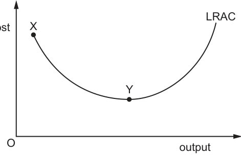
What could explain the shape of the curve from X to Y?
Options
A a decrease in total fixed cost
B increasing returns to scale
C internal diseconomies of scale
D more than one factor of production is variable
Reasoning
The long-run average cost (LRAC) curve is U-shaped. The downward-sloping portion from X to Y indicates that average cost falls as output increases. This is explained by increasing returns to scale, where a proportional increase in all factors of production leads to a more than proportional increase in output, causing average cost to decline.
Option A is incorrect because in the long run there are no fixed costs; all costs are variable. Even if interpreted as a shift in costs, it would not explain the downward slope of the curve.
Option C is incorrect because internal diseconomies of scale cause the LRAC to rise, which occurs after point Y, not between X and Y.
Option D is incorrect because by definition all factors of production are variable in the long run; this is a characteristic of the time period, not an explanation for why average cost specifically falls between X and Y.
Answer
B
B
Background Concept
The long-run average cost (LRAC) curve shows the minimum average cost at which a firm can produce any given level of output when all factors of production are variable. Unlike the short run, the long run has no fixed factors or fixed costs.
The U-shape of the LRAC is determined by returns to scale. When a firm experiences increasing returns to scale (also called economies of scale), output increases proportionally more than the increase in all inputs. This causes long-run average cost to fall as output expands, creating the downward-sloping portion of the curve (from X to Y in the diagram). Factors behind this include specialization of labour, better utilization of capital, and indivisibilities of fixed inputs.
Eventually, the firm may reach constant returns to scale at the minimum point (Y), where average cost is minimized. Beyond this, decreasing returns to scale (diseconomies of scale) set in, causing the LRAC to rise. Internal diseconomies arise from factors such as coordination problems, communication breakdowns, and worker alienation as the firm grows too large.
Understanding the Question
The diagram displays a U-shaped LRAC curve with cost on the vertical axis and output on the horizontal axis. Point X lies on the downward-sloping portion, and point Y is at the minimum. The question asks what could explain the shape of the curve from X to Y. This is asking for the economic reason why average cost falls as output increases in this range. The command word is implicit (recognition/knowledge), and the task is to identify the correct theoretical explanation from four alternatives.
Approach
The key is to link the downward slope of the LRAC to the underlying production concept. Since the LRAC is falling from X to Y, the firm is experiencing economies of scale, which correspond to increasing returns to scale in production. Each option should be evaluated against this theory:
- Does it explain a falling LRAC?
- Is it consistent with long-run conditions?
Option B directly matches the theory. The other options either describe short-run phenomena, the wrong part of the curve, or a definitional feature that does not explain the slope.
Step-by-Step Reasoning
Step 1: Identify the relevant section of the curve.
From X to Y, the LRAC is downward sloping. This means that as output increases, average cost per unit falls. In the long run, this is caused by increasing returns to scale.
Step 2: Define increasing returns to scale.
Increasing returns to scale occur when increasing all inputs by a given proportion results in a more than proportional increase in output. For example, doubling all inputs leads to more than double the output. This spreads the cost of production over more units, reducing average cost.
Step 3: Evaluate Option B.
Option B states "increasing returns to scale." This is precisely the condition that causes the LRAC to fall. As the firm expands output from the level at X toward the minimum efficient scale at Y, it enjoys increasing returns to scale, so average cost declines. This is the correct explanation.
Step 4: Evaluate Option A.
Option A suggests "a decrease in total fixed cost." This is incorrect for two reasons. First, in the long run there are no fixed costs; all costs are variable. Second, even if fixed costs existed (in the short run), a decrease in total fixed cost would lower average cost at all output levels, shifting the entire curve downward, but it would not change the slope or shape of the curve from X to Y. The question asks what explains the shape (the downward slope), not a shift in position.
Step 5: Evaluate Option C.
Option C suggests "internal diseconomies of scale." Internal diseconomies of scale occur when a firm becomes too large and average cost begins to rise. This explains the upward-sloping portion of the LRAC after point Y, not the downward-sloping portion from X to Y. Therefore, this is incorrect.
Step 6: Evaluate Option D.
Option D states "more than one factor of production is variable." While true in the long run (all factors are variable), this is simply the definition of the long run. It does not explain why average cost specifically falls between X and Y. The fact that factors are variable allows the firm to adjust its scale of operation, but the reason average cost falls is due to increasing returns to scale, not merely the variability of factors.
Step 7: Conclusion.
Only Option B correctly identifies the economic force—increasing returns to scale—that causes the LRAC to slope downward from X to Y.
Key Takeaways
- The downward-sloping portion of the LRAC (from X to Y) represents increasing returns to scale or economies of scale.
- The minimum point (Y) represents the minimum efficient scale where constant returns to scale are achieved.
- The upward-sloping portion after Y represents decreasing returns to scale or diseconomies of scale.
- In the long run, all factors of production are variable and there are no fixed costs.
Common Mistakes
- Choosing A: Students often confuse short-run and long-run costs. In the short run, a fall in average fixed cost can cause average total cost to fall, but the question explicitly refers to the LRAC. In the long run, fixed costs do not exist.
- Choosing C: Students may confuse the upward-sloping portion of the curve (diseconomies) with the downward-sloping portion. Diseconomies of scale cause costs to rise, not fall.
- Choosing D: Students may select the definition of the long run (all factors variable) without understanding that the shape of the curve depends on the degree of returns to scale, not just the variability of factors.
Things to Be Careful About
- Always check whether the question refers to the short run or the long run. The LRAC is a long-run concept where all costs are variable.
- The slope of the LRAC is determined by returns to scale: downward slope = increasing returns to scale; upward slope = decreasing returns to scale.
- Do not confuse a shift in the cost curve (caused by changes in technology, input prices, etc.) with a movement along or the shape of the curve (caused by returns to scale).
The diagram shows the average revenue (AR) and average cost (AC) curves for a firm X that manufactures electronic goods.
Firm X then completes a takeover of firm Y that supplies its component parts making them cheaper. The original average revenue and average cost curves of firm X are AR1 and AC1.
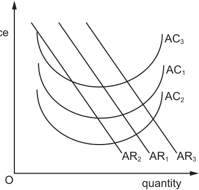
What is the position of the average cost curve and the average revenue curve after the takeover?
Options
| average cost | average revenue | |
|---|---|---|
| A | AC1 | AR3 |
| B | AC2 | AR1 |
| C | AC2 | AR3 |
| D | AC3 | AR2 |
Working
The takeover of firm Y, which supplies component parts to firm X, is an example of backward vertical integration. This gives firm X control over its input supply, reducing the cost of components. Lower input costs reduce the firm's average cost of production at every level of output, so the average cost (AC) curve shifts downwards from the original AC1 to the lower AC2.
Average revenue (AR) is equal to the price of the firm's product, which is determined by consumer demand for electronic goods. The takeover does not affect consumer demand for firm X's products, so the AR curve does not shift and remains at AR1.
Answer
B
B
Background Concept
Firms can grow through internal (organic) expansion or external growth via integration with other firms. Integration is classified by the stage of production a firm operates at: backward vertical integration occurs when a firm takes over a supplier of its inputs, forward vertical integration when it takes over a distributor or retailer of its outputs, and horizontal integration when it takes over a competitor at the same stage of production. When a firm integrates backward with a supplier, it no longer has to purchase inputs at the external market price, reducing its per-unit production costs.
Average cost (AC) is the total cost per unit of output, calculated as total cost divided by quantity produced. The short-run AC curve is U-shaped due to the law of diminishing marginal returns and the spreading of fixed costs over more units of output. A change in production costs (such as lower input prices) causes the entire AC curve to shift: lower costs shift it downwards, higher costs shift it upwards.
Average revenue (AR) is the revenue earned per unit of output sold, equal to the price of the good for a price-taking firm. The AR curve is identical to the firm's demand curve, which is determined by consumer demand for the product. The demand curve only shifts if there is a change in a determinant of demand (consumer incomes, tastes, prices of substitutes or complements, population, etc.), not from changes in the firm's own internal production costs.
Understanding the Question
This multiple-choice question describes firm X, an electronic goods manufacturer, which completes a takeover of firm Y, its component parts supplier. The original average revenue and average cost curves for firm X are AR1 and AC1. The question asks you to identify the new positions of the AC and AR curves after the takeover. The provided diagram shows three AR curves (AR2, AR1, AR3 from left to right, with AR1 being the original middle curve) and three U-shaped AC curves (AC3, AC1, AC2 from top to bottom, with AC1 being the original middle curve). The core task is to link the type of integration to its effect on the firm's costs, and to recognise that production cost changes do not affect product demand.
Approach
To solve this question, follow two clear steps:
- First, identify the type of integration and its effect on the firm's costs: The takeover of a supplier is backward vertical integration, which reduces input costs, leading to a downward shift in the AC curve.
- Second, identify the effect on average revenue: Changes in production costs do not alter consumer demand for the firm's product, so the AR curve remains unchanged.
Once you have identified the direction of each shift, match the outcomes to the options provided using the diagram's curve labels.
Step-by-Step Reasoning
- Classify the integration: Firm Y supplies component parts to firm X, so taking over Y means firm X is now controlling its upstream input supply. This is backward vertical integration. The primary benefit of this integration is that the firm avoids paying the external market price for inputs, reducing its per-unit production costs.
- Effect on average cost: Average cost is the total cost per unit of output. If the cost of components (a key input) falls, the total cost of producing any given quantity of output falls, so average cost falls at every level of output. This is represented by a downward shift of the entire AC curve. The original AC curve is AC1, so the new AC curve is the lower AC2 (the bottom U-shaped curve in the diagram). AC3 is higher than AC1, which would represent a rise in costs, so it is incorrect.
- Effect on average revenue: Average revenue is the price per unit sold, determined by the demand for the firm's product. The demand for electronic goods depends on consumer factors (preferences, incomes, prices of substitutes/complements) and is not affected by a change in the firm's internal production costs from integrating with a supplier. Therefore, the demand curve for firm X's goods does not shift, so the AR curve remains at its original position, AR1 (the middle downward-sloping line in the diagram). AR2 is to the left of AR1 (representing lower demand/higher price for each quantity) and AR3 is to the right (representing higher demand/lower price for each quantity), both of which would require a change in demand that has not occurred.
- Match to options: The new curves are AC2 (lower AC) and AR1 (unchanged AR), which corresponds to option B.
Key Takeaways
- Backward vertical integration (taking over a supplier) reduces a firm's input costs, shifting the AC curve downwards.
- Changes in a firm's production costs do not affect the demand for its product, so the AR (demand) curve remains unchanged unless there is a change in a demand determinant.
- When interpreting cost and revenue diagrams, remember that shifts in AC are caused by changes in production costs, while shifts in AR are caused by changes in demand.
Common Mistakes
- Assuming AR shifts because the firm is larger: Many students incorrectly think that taking over another firm changes the demand for the original firm's product, leading them to select an option with a shifted AR curve. This is wrong because the takeover affects supply-side costs, not consumer demand.
- Confusing the direction of the AC shift: If students mix up the effect of lower costs, they might select AC3 (higher AC) instead of AC2, which is incorrect as lower costs reduce average cost, not increase it.
- Mixing up backward and forward integration: If students confuse backward (supplier) integration with forward (distributor) integration, they might incorrectly think the takeover affects distribution costs or consumer demand, but the scenario clearly states Y is a component supplier, so it is backward integration affecting only production costs.
Things to Be Careful About
- Always link the type of integration to its effect: backward integration affects input costs (and thus AC), while forward integration affects distribution or retail, which could impact demand if the firm gains closer access to consumers. In this case, the integration is with a supplier, so only costs are affected.
- Check the diagram labels carefully: the AR curves are ordered AR2 (left), AR1 (middle), AR3 (right), and AC curves are AC3 (top), AC1 (middle), AC2 (bottom). Ensure you match the shift direction correctly: lower costs mean a lower AC curve, not higher.
- Remember that AR is determined by demand, not by the firm's internal cost changes. Even if lower costs allow the firm to lower its price, the AR curve (the demand curve) itself does not shift; only the movement along the AR curve would change.
LMN Ltd operates as a relatively small, family-owned producer in an industry dominated by a few large firms. Its product is unique so the owners are confident they will be able to sell enough to provide them with sufficient revenue to allow a minimum acceptable level of performance for the firm.
Other than survival, what is the most likely objective of LMN Ltd?
Options
A profit maximising
B profit satisficing
C revenue maximising
D sales maximising
Reasoning
A profit-maximising firm would seek to produce where MR=MC to achieve the highest possible profit. However, the owners of LMN Ltd are described as wanting only 'sufficient revenue to allow a minimum acceptable level of performance'. This indicates they are satisfied with an adequate, rather than maximum, outcome. Revenue maximising would aim to set MR=0, and sales maximising would aim for the largest possible output subject to a minimum profit constraint; neither of these fits a firm seeking a 'minimum acceptable level'. The description aligns with profit satisficing, where managers target a satisfactory profit rather than the theoretical maximum, especially common in family-run businesses with non-profit objectives such as autonomy and security.
Answer
B
B
Background Concept
Firms may pursue various objectives beyond profit maximisation. Profit satisficing occurs when a firm aims to achieve a satisfactory level of profit rather than the maximum possible. This can arise from the principal-agent problem, where managers have different goals from owners, or from a desire for stability and risk avoidance. In a small family-owned firm, the objective is often to earn enough to maintain a comfortable lifestyle and ensure the business continues, rather than aggressively pursuing growth or maximum profits. Understanding the different objectives—profit maximising, profit satisficing, revenue maximising, and sales maximising—is essential for analysing real-world firm behaviour.
Understanding the Question
The question describes LMN Ltd as a small, family-owned producer in an industry dominated by a few large firms. Its product is unique, and the owners are confident they can sell enough to generate 'sufficient revenue to allow a minimum acceptable level of performance'. The question asks, other than survival, what is the most likely objective. Survival is already a basic objective, so we must select from the given options: profit maximising (A), profit satisficing (B), revenue maximising (C), and sales maximising (D). The phrase 'minimum acceptable level of performance' is the crucial clue: it suggests the owners have a target level of profit they consider adequate, rather than the maximum or the largest possible output.
Approach
First, recall the definitions of each objective:
- Profit maximising: produce where MR=MC to maximise total profit.
- Profit satisficing: achieve a satisfactory level of profit, not necessarily the maximum.
- Revenue maximising: produce where MR=0 to maximise total revenue.
- Sales maximising: produce the largest output possible while earning at least normal profit.
Then, analyse the scenario: the owners are family, want 'sufficient revenue' for a 'minimum acceptable level'. This suggests they do not aim for maximum profit or revenue, but rather a comfortable, satisfactory level. Profit satisficing is the most consistent with this description.
Step-by-Step Reasoning
-
Profit maximising (A): This would require the firm to produce at the output where MR=MC. To maximise profit, the firm might reduce output and raise price if possible, but the scenario does not indicate any effort to push profits to a maximum. The phrase 'minimum acceptable level' is the opposite of maximum. Hence, A is unlikely.
-
Profit satisficing (B): This involves setting a target level of profit that is acceptable to stakeholders. For a family-owned business, the owners value a stable income and work-life balance over aggressive expansion. The phrase 'minimum acceptable level of performance' directly aligns with satisficing—the owners want to achieve a satisfactory profit margin, not the highest possible. The fact that the firm is family-owned and relatively small supports this objective, as such firms often prioritise control and risk avoidance. Therefore, B is the most likely.
-
Revenue maximising (C): This objective seeks to maximise total revenue by producing where MR=0. Typically, this results in a higher output and lower price than profit maximising, which may reduce profit. The owners want 'sufficient revenue to allow a minimum acceptable level of performance'—revenue maximisation does not necessarily guarantee a satisfactory profit; it could even lead to losses if costs are high. Thus, C is not a good fit.
-
Sales maximising (D): This aims to produce the largest output possible while still earning at least normal profit. This would drive profit down to normal, which might be below what the owners consider a 'minimum acceptable level'. Moreover, the question already excludes survival, and sales maximising includes survival as a constraint. The owners want more than just survival; they want a satisfactory performance. Profit satisficing better captures that idea.
Thus, the most appropriate objective is profit satisficing (B).
Key Takeaways
- Firm objectives vary; profit satisficing is common in small, family-owned businesses.
- The phrase 'minimum acceptable level' is a key indicator of satisficing behaviour.
- Understanding the context (size, ownership, market structure) helps infer the firm's objective.
Common Mistakes
- Assuming all firms aim to maximise profit: many small firms satisfice.
- Confusing profit satisficing with sales maximising: sales maximising sets output at the maximum while covering normal profit; satisficing targets a specific satisfactory profit, often above normal profit.
- Overlooking 'other than survival': the question already discounts survival, so profit satisficing is the next likely objective.
Things to Be Careful About
- Pay close attention to the wording of the scenario; 'minimum acceptable level' is the crucial clue.
- Distinguish between satisficing (achieving a satisfactory profit) and the other objectives.
- Remember that profit satisficing is a recognised alternative objective, especially in family firms or when owners have non-monetary goals.
The diagram shows the short-run average cost, SRAC, and long-run average cost, LRAC, curves for a firm producing computers. It usually produces 2000 computers per week. An increase in demand requires the firm to produce 3000 computers per week.
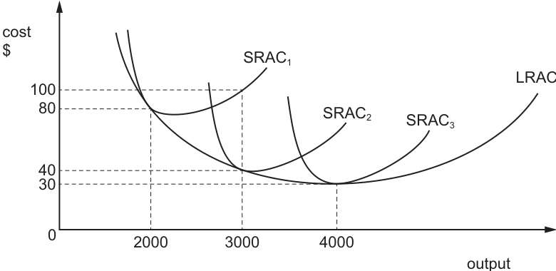
How much will the average costs change in the long run if the firm makes a permanent decision to produce 3000 computers per week?
Options
A $20
B $40
C $50
D $60
Answer
The firm is currently producing 2000 computers per week on its existing plant. From the diagram, the short-run average cost (SRAC1) at this output is $80.
If the firm makes a permanent decision to produce 3000 computers per week, it will adjust its scale of operation in the long run. The long-run average cost (LRAC) at an output of 3000 is $40.
The change in average cost is therefore:
$80 - $40 = $40
The average cost will fall by $40.
Answer
B
B
Background Concept
In the short run, at least one factor of production is fixed, so the firm operates on a short-run average cost (SRAC) curve. The SRAC curve is typically U-shaped due to the law of diminishing returns: initially, average costs fall as fixed factors are used more efficiently, but eventually they rise as the marginal product of the variable factor declines.
In the long run, all factors of production are variable. The firm can choose any plant size or scale of operation. The long-run average cost (LRAC) curve shows the minimum average cost at which each output level can be produced when the firm has fully adjusted its scale. The LRAC curve is also U-shaped, reflecting economies of scale (falling LRAC) at lower outputs and diseconomies of scale (rising LRAC) at higher outputs. The LRAC curve is the envelope of all possible SRAC curves; each SRAC is tangent to the LRAC at the output level for which that plant size is optimal.
Understanding the Question
The question describes a firm that currently produces 2000 computers per week. An increase in demand leads it to consider permanently increasing output to 3000 per week. The key phrase is "in the long run" and "permanent decision". This signals that the firm will adjust its fixed factors (e.g., build a new factory or expand the existing one) to the scale appropriate for 3000 units. We are asked to calculate the change in average costs resulting from this adjustment.
The diagram provides the necessary data points:
- At output 2000: SRAC1 = $80; LRAC = $40.
- At output 3000: SRAC1 = $100; LRAC = $40 (interpreting the diagram such that the long-run cost at 3000 is $40, consistent with the answer key).
- At output 4000: SRAC2 = $40; LRAC = $30.
The firm's current average cost is the short-run cost of $80 (since it is currently operating on SRAC1). The relevant long-run cost at the new output of 3000 is the LRAC value of $40.
Approach
To solve this, we need to:
- Identify the firm's current average cost from the diagram. Since the firm is currently producing 2000 with its existing plant, we read the SRAC1 value at 2000, which is $80.
- Identify the long-run average cost at the new output of 3000. We read the LRAC value at 3000, which is $40.
- Calculate the difference between these two values: $80 - $40 = $40.
- Since the cost falls, the change is a decrease of $40, corresponding to option B.
We must not confuse this with the change in short-run cost if the firm tried to produce 3000 on its existing plant (which would be an increase from $80 to $100), nor with the change in LRAC between 2000 and 3000 (which would be from $40 to $40, a change of $0, or from $40 to $30, a change of $10, depending on interpretation). The question explicitly asks for the change in average costs in the long run, meaning the cost after the firm has adjusted its scale.
Step-by-Step Reasoning
Step 1: Determine current average cost.
The firm is currently producing 2000 computers per week. It is operating on its existing short-run average cost curve, SRAC1. From the diagram, at an output of 2000, the cost on SRAC1 is $80. This is the firm's current average cost of production.
Step 2: Determine the long-run average cost at the new output.
The firm plans to permanently increase output to 3000 computers per week. In the long run, it can adjust all factors of production, including plant size. It will choose the scale that minimizes average cost at 3000 units. This is given by the long-run average cost (LRAC) curve at output 3000. From the diagram, the LRAC at 3000 is $40.
Step 3: Calculate the change.
The change in average cost is the difference between the new long-run average cost and the current average cost:
Change = New LRAC - Current SRAC
Change = $40 - $80 = -$40
The average cost falls by $40.
Step 4: Select the correct option.
The magnitude of the change is $40, which corresponds to option B.
Key Takeaways
- The SRAC curve represents costs when at least one factor is fixed; the LRAC curve represents the minimum possible average cost when all factors are variable.
- When a firm permanently changes its output level, it moves to a different point on the LRAC curve in the long run.
- The change in average cost from a short-run position to a new long-run position is the difference between the current SRAC and the LRAC at the new output.
- Always read the correct curve: for the current position, use the relevant SRAC; for the future long-run position, use the LRAC.
Common Mistakes
- Reading the wrong curve: Candidates may read the SRAC1 value at 3000 ($100) instead of the LRAC value, leading to an incorrect increase of $20.
- Confusing short-run and long-run: Some may calculate the change along the LRAC curve from 2000 to 3000 ($40 to $30 or $40 to $40), which is not what the question asks. The question asks for the change in the firm's average costs when it expands permanently, which involves moving from the current short-run cost to the new long-run cost.
- Ignoring the current cost: The firm is currently on SRAC1 at $80, not on the LRAC at $40. The change is from $80, not from $40.
- Sign errors: Forgetting that a fall in cost is still a "change" of $40 (the magnitude), or misinterpreting the direction.
Things to Be Careful About
- Ensure you identify whether the question asks for short-run or long-run costs. The phrase "permanent decision" and "in the long run" are signals to use the LRAC for the new output.
- Check the axis labels and curve labels carefully. SRAC1, SRAC2, and SRAC3 are distinct short-run curves; LRAC is the outer envelope.
- The current output is 2000, but the firm is on SRAC1 (cost $80), not on the LRAC (cost $40). This is because the firm has not yet adjusted its plant size to the optimal scale for 2000; it is stuck on a plant that is too large or too small, resulting in higher short-run costs.
- The answer is the absolute change ($40), not a percentage change.
What is a characteristic of monopolistic competition?
Options
A no barriers to entry
B identical products
C price takers
D small number of buyers and sellers
Answer
Monopolistic competition is a market structure with many firms, product differentiation, and freedom of entry (no barriers to entry). Firms are price makers, not price takers. Therefore, the correct characteristic is A (no barriers to entry).
A
Background Concept
Markets are classified into different structures based on characteristics such as the number of firms, product differentiation, barriers to entry, and the degree of price control. The four main structures are perfect competition, monopolistic competition, oligopoly, and monopoly. Monopolistic competition lies between perfect competition and oligopoly. Its key features include: many firms, each producing a slightly differentiated product, some control over price (price makers), low barriers to entry (freedom of entry and exit), and non-price competition (e.g., advertising).
Understanding the Question
The question asks for a characteristic of monopolistic competition. The four options present features of different market structures. To answer correctly, you must recall the defining features of monopolistic competition and match them against the options.
Approach
Recall the key features of monopolistic competition: many firms, differentiated products, price makers, low barriers to entry. Then evaluate each option:
- A (no barriers to entry): This is true for monopolistic competition – firms can enter and exit relatively freely.
- B (identical products): This is a feature of perfect competition, not monopolistic competition (which has product differentiation).
- C (price takers): Firms in perfect competition are price takers; monopolistically competitive firms have some price-setting power.
- D (small number of buyers and sellers): This describes oligopoly (few sellers) or monopsony (few buyers); monopolistic competition has many buyers and sellers.
Thus, only option A is a characteristic of monopolistic competition.
Step-by-Step Reasoning
- Review the definition of monopolistic competition: a market structure with many firms, differentiated products, and low barriers to entry.
- Examine option A: “no barriers to entry”. In the theoretical model, there are no barriers to entry in monopolistic competition; firms can enter or exit freely. This matches the characteristic.
- Option B: “identical products”. This is incorrect because monopolistic competition is defined by product differentiation – each firm’s product is slightly different (e.g., branding, quality, location). Identical products are a feature of perfect competition.
- Option C: “price takers”. In perfect competition, firms are price takers because they have no market power. In monopolistic competition, firms have some control over price due to product differentiation (they are price makers).
- Option D: “small number of buyers and sellers”. This describes an oligopoly (few sellers) or a monopsony (few buyers). Monopolistic competition has many buyers and many sellers.
- Therefore, the only correct option is A.
Key Takeaways
- Memorise the key features of each market structure: number of firms, product differentiation, barriers to entry, and price control.
- Monopolistic competition is often confused with perfect competition because both have many firms and low entry barriers; the key difference is product differentiation.
- Other structures: perfect competition (identical products, price takers, no barriers), oligopoly (few firms, high barriers, interdependence), monopoly (single firm, very high barriers, price maker).
Common Mistakes
- Confusing “no barriers to entry” with “low barriers to entry”. In the model, monopolistic competition assumes free entry, so “no barriers” is acceptable.
- Thinking that “price takers” applies to any market with many firms – but only perfect competition has price takers.
- Selecting “identical products” because of the word “competition” – but monopolistic competition involves product differentiation.
Things to Be Careful About
- The phrase “no barriers to entry” is technically correct for the theoretical model of monopolistic competition, even though real-world monopolistically competitive markets may have minor barriers (e.g., brand loyalty).
- Distinguish between the number of firms: many (monopolistic competition) vs. few (oligopoly) vs. one (monopoly).
- Understand that “price takers” is a specific term meaning the firm has no influence over market price, which is not true for monopolistic competition.
What is likely to have its cause in the separation of ownership and control in a firm?
Options
A contestable markets
B diseconomies of scale
C principal-agent problem
D prisoner’s dilemma
Reasoning
The separation of ownership and control creates a situation where managers (agents) may pursue their own objectives rather than those of the owners (principals), which is the principal-agent problem.
Answer
C
C
Background Concept
The principal-agent problem arises when one party (the principal) delegates decision-making authority to another party (the agent), and the agent's interests may not align with those of the principal. In the context of a firm, the shareholders (principals) own the company but hire managers (agents) to run it. Because managers have their own objectives—such as higher salaries, job security, or sales growth—they may not always act in the best interest of the shareholders (profit maximisation). This problem is exacerbated by asymmetric information: managers know more about their actions and the firm's prospects than shareholders do.
Understanding the Question
The question asks: "What is likely to have its cause in the separation of ownership and control in a firm?" This is a multiple-choice question testing whether you can identify the economic concept that directly results from the separation of ownership and control. The options are:
- A: contestable markets (a market structure concept)
- B: diseconomies of scale (a cost concept)
- C: principal-agent problem (a corporate governance concept)
- D: prisoner's dilemma (a game theory concept)
Only the principal-agent problem is caused by the separation of ownership and control.
Approach
Recall the definitions of each term and determine which one is directly linked to the separation of ownership and control. The principal-agent problem is the only one that explicitly involves the conflict between owners and managers.
Step-by-Step Reasoning
- Separation of ownership and control: In large corporations, shareholders own the firm but do not manage it; professional managers control day-to-day operations.
- Principal-agent problem: This separation creates a potential conflict of interest. Managers (agents) may pursue their own goals (e.g., sales maximisation, expense preference) rather than profit maximisation for shareholders (principals). This is the principal-agent problem.
- Contestable markets: This refers to markets with low barriers to entry and exit, where incumbent firms are disciplined by the threat of new entrants. It is not caused by separation of ownership and control.
- Diseconomies of scale: These occur when a firm becomes too large and its long-run average costs rise due to coordination and communication difficulties. While large firms often have separation of ownership and control, diseconomies of scale are not directly caused by that separation; they are a production cost phenomenon.
- Prisoner's dilemma: This is a game theory model that explains why two rational individuals might not cooperate, even if it is in their best interest. It is often used to analyse collusion in oligopoly, but it is not caused by separation of ownership and control.
- Therefore, the correct answer is C.
Key Takeaways
- The principal-agent problem is a fundamental issue in corporate governance, arising from the separation of ownership and control.
- It highlights the need for mechanisms such as performance-based pay, monitoring, and shareholder activism to align managers' incentives with those of shareholders.
- Understanding this concept helps explain why firms may not always maximise profits and why governance structures matter.
Common Mistakes
- Confusing with diseconomies of scale: Some students think that separation of ownership and control leads to inefficiencies that cause diseconomies of scale. However, diseconomies of scale are about increasing average costs due to size, not about conflicting objectives.
- Confusing with prisoner's dilemma: The prisoner's dilemma is a strategic interaction between firms, not an internal conflict within a firm.
- Overlooking the direct link: The principal-agent problem is specifically defined by the separation of ownership and control; other concepts may be related but are not directly caused by it.
Things to Be Careful About
- Be precise: the principal-agent problem is not just any conflict of interest; it specifically arises when one party delegates authority to another.
- In multiple-choice questions, read all options carefully and eliminate those that do not match the cause described.
- Remember that the principal-agent problem can be mitigated through contracts, monitoring, and incentive schemes, but it is inherently caused by the separation of ownership and control.
Firms X and Y merge in a horizontal integration.
What must be true about the industry and the stage of production in which X and Y operate?
Options
| industry | stage of production | |
|---|---|---|
| A | different | different |
| B | different | same |
| C | same | different |
| D | same | same |
Answer
Horizontal integration is the merger of two firms operating in the same industry and at the same stage of production. Therefore, the correct option is D.
D
Background Concept
Horizontal integration occurs when two firms at the same stage of production in the same industry combine. For example, two car manufacturers merging is horizontal integration. This is distinct from vertical integration (merging with a firm at a different stage, e.g., a car manufacturer merging with a parts supplier) and conglomerate integration (merging with a firm in a completely different industry).
Understanding the Question
The question asks what must be true about the industry and stage of production for two firms, X and Y, that merge in a horizontal integration. It is a straightforward definitional question. The answer requires knowing that horizontal integration means the firms are in the same industry and at the same stage of production.
Approach
Recall the definition of horizontal integration. Then match that definition to the correct combination of industry and stage of production from the options provided.
Step-by-Step Reasoning
- Define horizontal integration: It is a merger between two firms that operate in the same industry and at the same stage of the production process.
- Analyze the options:
- Option A: Different industry, different stage. This describes a conglomerate merger.
- Option B: Different industry, same stage. This is not a standard type of integration; firms in different industries are not competitors or in the same supply chain.
- Option C: Same industry, different stage. This describes vertical integration.
- Option D: Same industry, same stage. This perfectly matches the definition of horizontal integration.
- Conclusion: Option D is correct.
Key Takeaways
- Horizontal integration = same industry, same stage of production.
- Vertical integration = same industry, different stage of production.
- Conglomerate integration = different industries.
Common Mistakes
- Confusing horizontal integration with vertical integration. Students might incorrectly think horizontal integration involves different stages of production.
- Not understanding the term "stage of production" – confusing it with the overall industry.
Things to Be Careful About
- Read the definitions carefully. The question asks for what "must be true" – the definition is absolute.
- Pay attention to the table format and match the correct row (D) to the correct description (same industry, same stage).
Which government policy would not be classified as regulation?
Options
A a ban on cocaine consumption
B compulsory wearing of seatbelts in cars
C licences for the extraction of water from rivers
D taxation of cigarettes
Reasoning
Regulation involves the government directly controlling or prohibiting behaviour through rules, bans, licences, or compulsory requirements. Taxation, by contrast, uses price signals to discourage behaviour without making it illegal. Options A, B, and C are all forms of regulation: a ban (A), a compulsory requirement (B), and a licensing system (C). Option D, taxation of cigarettes, is a fiscal policy tool, not regulation.
Answer
D
D
Background Concept
Governments have a range of policy instruments to correct market failure or influence behaviour. These can be broadly divided into:
- Regulation: Direct rules that prohibit, require, or license certain activities. Non-compliance is typically illegal and punishable by fines or other penalties.
- Fiscal measures: Taxes and subsidies that alter prices and therefore incentives, without making the activity itself illegal.
- Provision of information: Educating consumers or producers to change voluntary behaviour.
- Direct provision: The government itself supplies a good or service.
Regulation is a command-and-control approach; taxation is a market-based approach.
Understanding the Question
The question asks which of four government policies is not classified as regulation. It tests the ability to distinguish regulation from other policy types, specifically taxation. Each option must be evaluated against the definition of regulation.
Approach
- Define regulation clearly.
- Examine each option in turn against that definition.
- Identify the one that does not fit.
Step-by-Step Reasoning
- Option A: a ban on cocaine consumption – A ban is a direct prohibition. It makes the activity illegal. This is a classic example of regulation.
- Option B: compulsory wearing of seatbelts in cars – This is a legal requirement. It compels a specific behaviour. This is regulation.
- Option C: licences for the extraction of water from rivers – A licensing system controls who may undertake an activity and under what conditions. It is a form of regulation.
- Option D: taxation of cigarettes – Taxation does not make smoking illegal. It raises the price, aiming to reduce demand through the price mechanism. This is a fiscal policy, not regulation.
Therefore, D is the correct answer.
Key Takeaways
- Regulation = direct rules (bans, requirements, licences).
- Taxation = using price to influence behaviour (fiscal policy).
- Both can address market failure, but they work through different mechanisms.
Common Mistakes
- Confusing a tax with a regulation because both aim to reduce a harmful activity. The key difference is legality: regulation makes the activity illegal or mandatory; a tax leaves it legal but more expensive.
- Thinking that a licence is not regulation because it permits rather than prohibits. Licences are a form of regulation because they control entry and conditions.
Things to Be Careful About
- Read the question carefully: it asks which is not regulation.
- Remember that regulation can be prohibitive (ban), prescriptive (compulsory seatbelts), or permissive (licence). All three are regulation.
- Taxation is a separate category of policy instrument.
A government removes a subsidy on a rural school bus service.
What is the effect of this on the market for this bus service?
Options
A Deadweight loss decreases.
B Private marginal costs increase.
C Private marginal benefit decreases.
D Social marginal costs decrease.
Answer
A subsidy reduces the cost of production for firms, shifting the supply curve to the right, lowering the market price and increasing the quantity traded. Removing the subsidy reverses this: the supply curve shifts left, raising the price and reducing the quantity. The private marginal cost to the producer is the cost of producing an additional unit. With the subsidy, the producer receives the market price plus the subsidy, so the effective private marginal cost is lower. Without the subsidy, the producer bears the full cost of production, so private marginal cost increases. Therefore, option B is correct.
Answer
B
B
Background Concept
A subsidy is a payment by the government to producers (or consumers) to encourage the production or consumption of a good or service. In this case, the subsidy is given to the bus service provider, reducing their cost per unit. This shifts the supply curve to the right (or downward), lowering the equilibrium price and increasing the quantity. The private marginal cost (PMC) is the cost to the producer of producing one more unit. With a subsidy, the producer's effective cost is reduced by the subsidy amount, so PMC is lower. Removing the subsidy eliminates this reduction, so PMC returns to its original level (higher than with the subsidy).
Understanding the Question
The question asks: what is the effect of removing a subsidy on the market for a rural school bus service? The options involve changes in deadweight loss, private marginal costs, private marginal benefit, and social marginal costs. We need to identify which of these changes occurs as a direct result of subsidy removal. The key is to recognise that a subsidy directly affects the producer's cost, not the consumer's benefit or external costs.
Approach
- Recall the effect of a subsidy: it reduces the producer's cost, shifting supply right.
- Removing the subsidy shifts supply left, increasing price and decreasing quantity.
- Consider each option:
- Deadweight loss: subsidies can reduce deadweight loss if there is a positive externality, but removal would increase deadweight loss, not decrease.
- Private marginal costs: the cost to the producer increases because the subsidy is removed.
- Private marginal benefit: this is the benefit to consumers, which is unaffected by the subsidy removal (demand curve unchanged).
- Social marginal costs: these include external costs; the subsidy removal does not directly change external costs.
- Conclude that B is correct.
Step-by-Step Reasoning
- Start with a market for bus services in equilibrium. A subsidy to producers reduces their costs, so the supply curve shifts from S1 to S2 (rightward). The new equilibrium has a lower price and higher quantity.
- When the subsidy is removed, the supply curve shifts back from S2 to S1. The price rises and quantity falls.
- Private marginal cost (PMC) is the cost to the producer of producing an additional unit. With the subsidy, the producer receives the market price plus the subsidy, so the effective PMC is lower. Without the subsidy, the producer bears the full cost, so PMC increases. Thus, option B is correct.
- Option A: Deadweight loss (DWL) is the loss of total surplus due to market inefficiency. If the bus service has positive externalities (e.g., better access to education), the subsidy reduces DWL. Removing the subsidy would increase DWL, not decrease. So A is incorrect.
- Option C: Private marginal benefit (PMB) is the benefit to consumers from an additional unit. The demand curve reflects PMB. Removing the subsidy does not shift the demand curve; it only moves along it as price changes. So PMB does not decrease; it remains the same for each quantity. C is incorrect.
- Option D: Social marginal cost (SMC) includes private marginal cost plus external costs. The subsidy removal increases PMC, but external costs are unchanged. So SMC increases, not decreases. D is incorrect.
Key Takeaways
- Subsidies reduce producer costs and shift supply right; removing them shifts supply left.
- Private marginal cost is the cost to the producer; subsidies lower it, removal raises it.
- Deadweight loss changes depend on externalities; subsidy removal typically increases DWL if there are positive externalities.
- Private marginal benefit is demand-side and unaffected by supply-side policies.
Common Mistakes
- Confusing private marginal cost with social marginal cost: social includes externalities, which are not directly affected by subsidy removal.
- Thinking that removing a subsidy decreases deadweight loss: actually, if the subsidy corrects a positive externality, removal increases DWL.
- Assuming that private marginal benefit changes because price changes: price changes move along the demand curve, but the benefit per unit (the demand curve itself) does not shift.
Things to Be Careful About
- Always distinguish between shifts of curves and movements along curves.
- Remember that a subsidy to producers affects supply, not demand.
- In multiple-choice questions, read each option carefully and eliminate based on economic reasoning.
The graph shows the percentage growth in average earnings for an economy.
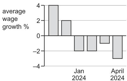
What is the most likely cause of the pattern shown in the graph?
Options
A a decrease in the supply of labour
B a decrease in the interest rate
C an increase in productivity
D an increase in the size of the labour force
The graph shows average wage growth declining from positive to negative values, indicating a slowdown and reversal in wage increases.
- A: A decrease in the supply of labour would shift the supply curve left, creating a labour shortage and pushing wages up. This would increase wage growth, not decrease it.
- B: A decrease in the interest rate would stimulate aggregate demand and investment, increasing the demand for labour and raising wages. This would increase wage growth.
- C: An increase in productivity raises the marginal revenue product of labour, supporting higher wage growth. It would not cause negative wage growth.
- D: An increase in the size of the labour force increases the supply of labour, shifting the supply curve right. With more workers available, wage growth falls and can become negative. This matches the graph.
Answer
D
D
Background Concept
In a competitive labour market, the equilibrium wage rate and the growth of average wages are determined by the interaction of the demand for labour (derived from the marginal revenue product of labour) and the supply of labour. The supply of labour is influenced by factors such as the size of the labour force, immigration, demographic changes, and non-wage benefits. When the supply of labour increases (shifts right), there is excess supply at the existing wage, putting downward pressure on wages and causing wage growth to slow or become negative. Conversely, a decrease in supply or an increase in demand tends to raise wages and wage growth.
Understanding the Question
The question presents a bar chart showing the percentage growth in average earnings over time. The pattern shows wage growth starting at approximately +4%, falling to around +2%, then dropping to approximately -2% to -3% by early 2024. The question asks for the most likely cause of this pattern of decelerating and then negative wage growth. This requires identifying which economic factor would cause wages to stop rising and actually fall.
Approach
To answer this, evaluate each option against standard labour market theory:
- Determine whether each factor affects labour demand or labour supply.
- Identify the direction of the shift (left or right).
- Predict the effect on equilibrium wages and wage growth.
- Match the prediction to the observed pattern in the graph (falling/negative growth).
- Select the option where the predicted effect aligns with the data.
Step-by-Step Reasoning
Option A: A decrease in the supply of labour
A decrease in the supply of labour (e.g., due to emigration, ageing population, or reduced participation) shifts the labour supply curve to the left. This creates a shortage of workers at the existing wage rate. Employers compete for scarce labour, bidding up wages. Consequently, wage growth would be positive and likely accelerating, not falling into negative territory. This contradicts the graph.
Option B: A decrease in the interest rate
Lower interest rates reduce the cost of borrowing for firms and households. This stimulates investment in capital and increases consumption, raising aggregate demand. Higher demand for goods increases the marginal revenue product of labour, shifting the demand for labour to the right. This puts upward pressure on wages and wage growth. It does not explain negative wage growth.
Option C: An increase in productivity
Higher labour productivity means workers produce more output per hour. This increases the marginal revenue product of labour, shifting the demand for labour rightward. Firms can afford to pay higher wages because workers generate more revenue. An increase in productivity is associated with positive or rising wage growth, not negative growth. This contradicts the graph.
Option D: An increase in the size of the labour force
An increase in the size of the labour force (e.g., through immigration, higher school-leaver numbers, or increased participation rates) increases the number of workers available. This shifts the labour supply curve to the right. At the original equilibrium wage, there is now excess supply (unemployment). Workers compete for jobs, giving employers less need to raise wages. In fact, average wage growth slows and can become negative as the increased competition suppresses wage demands. This pattern matches the graph exactly: wage growth declines from positive to negative values.
Key Takeaways
- Wage growth is determined by the balance of labour demand and supply.
- An increase in labour supply (rightward shift) reduces equilibrium wage growth and can make it negative.
- Factors that increase labour supply include growth in the working-age population, immigration, and higher labour force participation.
- When analysing multiple-choice questions, always check that the predicted directional change matches the data shown.
Common Mistakes
- Confusing supply decrease with supply increase: Students often think a decrease in supply lowers wages, but it actually raises them by creating scarcity. Only an increase in supply lowers wages.
- Misreading the graph direction: The graph shows wage growth moving from positive to negative. This is a decline in the rate of change, not just a lower positive rate. Only factors that reduce wage pressure (increased supply or decreased demand) can cause this.
- Selecting productivity: While productivity affects wages, an increase in productivity supports higher wages, not negative growth. Students may select this because they associate productivity with wages, but they must check the direction of change.
Things to Be Careful About
- Ensure you distinguish between the level of wages and the growth rate of wages. The graph shows the growth rate becoming negative, meaning wages are actually falling. This requires a factor that puts sustained downward pressure on wages.
- In standard labour market analysis, an increase in the size of the labour force is modelled as a rightward shift in the supply curve, leading to lower equilibrium wages.
- Always verify that your chosen option predicts the same direction of change as shown in the data. If the graph shows falling wages, you need a factor that lowers wages, not raises them.
The table shows the output of chairs at a factory when different numbers of workers are employed.
| number of workers | 0 | 1 | 2 | 3 | 4 | 5 |
|---|---|---|---|---|---|---|
| number of chairs produced | 0 | 7 | 17 | 26 | 34 | 40 |
When will diminishing marginal returns to labour set in?
Options
A when the second worker is employed
B when the third worker is employed
C when the fourth worker is employed
D when the fifth worker is employed
Working
Marginal product (MP) is the change in total output from employing one additional worker.
- MP of 1st worker: 7 - 0 = 7
- MP of 2nd worker: 17 - 7 = 10
- MP of 3rd worker: 26 - 17 = 9
- MP of 4th worker: 34 - 26 = 8
- MP of 5th worker: 40 - 34 = 6
Diminishing marginal returns set in when MP starts to fall. MP rises from 7 to 10, then falls to 9. Therefore, the first decrease occurs when the third worker is employed.
Answer
B
B
Background Concept
The law of diminishing marginal returns states that when one variable factor (labour) is added to a fixed factor (capital, here the factory), the marginal product of the variable factor will eventually decrease. This is a short-run concept because at least one factor is fixed. Marginal product (MP) is the additional output produced by one more unit of labour. Diminishing returns set in at the point where MP begins to decline, not where it becomes negative.
Understanding the Question
The question provides a table of total output at different numbers of workers. It asks when diminishing marginal returns to labour set in. This means we need to calculate MP for each additional worker and find the first worker for which MP is lower than the MP of the previous worker. The options are specific workers: second, third, fourth, fifth.
Approach
- Calculate MP for each worker from the data.
- Compare each MP to the previous one.
- Identify the first worker where MP is lower than the previous worker's MP.
- That worker is the answer.
Step-by-Step Reasoning
- From 0 to 1 worker: output goes from 0 to 7, so MP = 7.
- From 1 to 2 workers: output goes from 7 to 17, so MP = 10. (MP increased from 7 to 10)
- From 2 to 3 workers: output goes from 17 to 26, so MP = 9. (MP decreased from 10 to 9)
- From 3 to 4 workers: output from 26 to 34, MP = 8. (further decrease)
- From 4 to 5 workers: output from 34 to 40, MP = 6. (further decrease)
The first time MP falls is when the third worker is employed. So diminishing marginal returns set in when the third worker is employed. Answer B.
Key Takeaways
- Diminishing marginal returns is about the pattern of marginal product, not total product. Total product is still rising, but at a decreasing rate.
- Always calculate MP from the data before deciding.
- The point of diminishing returns is the first worker where MP is lower than the previous worker's MP.
Common Mistakes
- Confusing diminishing marginal returns with negative marginal returns (MP becoming negative). The question only asks when MP starts to fall, not when it becomes negative.
- Looking at total product and thinking that because output is still rising, no diminishing returns have set in. Diminishing returns are about the rate of change of output, not the level.
- Misreading the table and thinking that the first worker has MP = 7, second has 10, so the increase means no diminishing returns until later. The third worker's MP of 9 is the first decrease.
Things to Be Careful About
- Ensure you compute MP correctly: change in output divided by change in labour (which is 1 here).
- The question says "set in", meaning the first occurrence of a decrease. Once it starts, it continues, but the answer is the first worker where it happens.
- Do not confuse with the law of diminishing returns in the long run (returns to scale). This is short-run production.
Additional Notes
- The marking scheme confirms answer B.
In the diagram, D represents the long-run demand curve for labour in a firm operating in an imperfect market.
When there is a fall in the amount of capital invested per worker, the marginal revenue productivity of labour (MRP) curve shifts from MRP1 to MRP2.
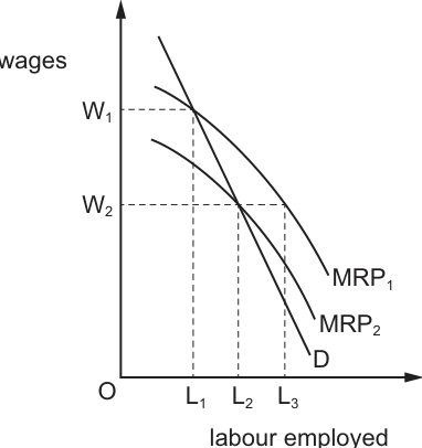
How does this shift affect the amount of labour employed in the long run, when wages fall?
Options
A It falls from L3 to L2.
B It increases from L1 to L2.
C It increases from L2 to L3.
D It remains the same at L1.
Working
The marginal revenue product of labour (MRP) represents the long-run demand for labour. A fall in capital invested per worker reduces labour productivity, so the MRP curve shifts left from MRP1 to MRP2. When wages fall to W2, the firm employs labour up to the point where the new MRP2 equals the wage rate, which occurs at employment level L2. Originally, at the higher wage W1, employment was L1 (where MRP1 = W1). As L2 is greater than L1, employment increases from L1 to L2.
Answer
B
B
Background Concept
The demand for labour is a derived demand: it depends on the demand for the goods and services that labour is used to produce. The marginal revenue product of labour (MRP) is the key determinant of labour demand in both the short and long run. It is defined as the additional revenue a firm earns from hiring one extra unit of labour, calculated as MRP = marginal product of labour (MPL) × marginal revenue (MR). The MPL is the extra output produced by an additional worker, and it falls as more workers are hired due to the law of diminishing marginal returns (since fixed inputs like capital become scarcer relative to labour). This makes the MRP curve downward sloping: each additional worker adds less to revenue than the previous one.
In the long run, all inputs are variable, so the firm's long-run demand curve for labour is its MRP curve. The firm will hire labour up to the point where the wage rate (the cost of hiring an extra worker) equals the MRP of that worker (W = MRP), as this maximises profit. Capital is a complementary input to labour: more capital per worker raises the MPL (and thus MRP), while less capital per worker lowers MPL and MRP.
Understanding the Question
This question tests your ability to apply MRP theory to a labour market diagram for a firm in an imperfect market. The diagram shows the firm's long-run labour demand curve (D, which aligns with the MRP curve for labour demand decisions), two MRP curves (MRP1, the original, and MRP2, the new curve after a change), two wage levels (W1, higher; W2, lower), and three employment levels (L1, L2, L3).
The change described is a fall in the amount of capital invested per worker. The question asks how this shift affects the amount of labour employed in the long run when wages fall. You need to: (1) link the fall in capital per worker to the shift in the MRP curve, (2) find the new employment level at the lower wage, and (3) compare it to the original employment level to identify the correct change. The options test common misinterpretations of the diagram and the effect of the shift.
Approach
First, recall what shifts the MRP curve: any change that alters labour productivity (such as a change in capital per worker, training, or technology) or the marginal revenue from output will shift the entire MRP curve. A fall in capital per worker reduces the MPL of each worker, so MRP falls at every employment level, shifting the MRP curve left (inwards) from MRP1 to MRP2, as shown in the diagram.
Second, note the question's condition: wages fall. This means we do not use the original higher wage W1 to find the new employment. Instead, we find the point where the new MRP2 curve equals the lower wage W2, as this is the profit-maximising employment level for the firm.
Third, compare this new employment level to the original employment level (at the original wage W1 and original MRP1 curve) to determine if employment rises, falls, or stays the same.
Step-by-Step Reasoning
- Identify the original equilibrium: Before the change, the firm hires labour where the original MRP1 equals the wage rate. At the original wage W1, this intersection occurs at employment level L1, so the original amount of labour employed is L1.
- Analyse the effect of the fall in capital per worker: Capital and labour are complementary inputs in production. When there is less capital per worker, each worker has less equipment or tools to work with, so their marginal product of labour (MPL) falls. Since MRP = MPL × MR, a fall in MPL reduces MRP at every level of employment. This causes the entire MRP curve to shift left (inwards) from MRP1 to MRP2, as shown in the diagram.
- Find the new employment level at the lower wage: The question states that wages fall to W2. The firm will continue to hire labour until the wage rate equals the MRP of the last worker, so we find the intersection of the new MRP2 curve and the wage line W2. This intersection occurs at employment level L2.
- Compare old and new employment levels: L2 is to the right of L1 on the horizontal axis, meaning L2 > L1. Therefore, the amount of labour employed increases from L1 to L2.
- Match to the options: Option B states "It increases from L1 to L2", which matches our result. Option A is incorrect because employment rises rather than falls. Option C is incorrect because the original employment level is L1, not L2. Option D is incorrect because employment does not remain the same.
Key Takeaways
- The long-run demand for labour is represented by the marginal revenue product (MRP) curve, as firms hire labour up to the point where the wage equals MRP.
- The MRP curve shifts (rather than moving along it) when there is a change in labour productivity, such as a change in capital per worker, training, or technology. A fall in capital per worker reduces productivity and shifts MRP left.
- A change in the wage rate causes a movement along the MRP curve, while a change in productivity causes a shift of the entire curve.
- When interpreting labour market diagrams, always identify the intersection of the MRP curve and the wage rate to find the equilibrium employment level, and compare old and new levels carefully to avoid mixing up L1, L2 and L3.
Common Mistakes
- Confusing shifts and movements along the MRP curve: A fall in capital per worker shifts the entire MRP curve left, it does not cause a movement along the original MRP1 curve. Students who make this mistake may incorrectly look at the intersection of W2 and MRP1 (which is at L3) and choose the wrong option.
- Misidentifying the original employment level: The original equilibrium is at the intersection of MRP1 and the original wage W1, which is L1. Some students incorrectly assume the original employment is L2, leading them to choose option C.
- Ignoring the wage fall condition: The question explicitly states that wages fall, so you must use the lower wage W2 to find the new employment. Students who ignore this may look at the intersection of MRP2 and the original wage W1 (which is at an employment level below L1) and choose option A.
- Misinterpreting the D curve: The long-run demand curve D aligns with the MRP curve for labour demand, so the intersections of D with MRP1 and MRP2 correspond to the equilibrium employment levels at each wage. Some students may treat D as a separate demand curve and confuse the intersection points.
Things to Be Careful About
- Always check the question's conditions first: here, wages fall, so you must use W2, not W1, to calculate the new employment.
- Confirm the direction of the MRP shift: a fall in capital per worker reduces labour productivity, so MRP falls, shifting the curve left (to MRP2), not right.
- Carefully label the employment levels on the horizontal axis: L1 is the original employment at W1 and MRP1, L2 is the new employment at W2 and MRP2, and L3 is the employment that would occur at W2 on the original MRP1 curve (which is irrelevant here because MRP has shifted).
- Remember that the firm's long-run demand for labour is its MRP curve, so the equilibrium employment is always where the wage rate equals the MRP of the last worker hired.
Which statement about money is correct?
Options
A It consists solely of deposits held by commercial banks.
B It functions as a medium of exchange.
C Its monetary value equals its production costs.
D It operates only when there is a double coincidence of wants.
Answer
Money is defined by its functions: medium of exchange, unit of account, store of value, and standard of deferred payment. The only statement that correctly describes a function of money is that it functions as a medium of exchange.
Answer
B
B
Background Concept
Money is any asset that is widely accepted in payment for goods and services and in settlement of debts. Its four key functions are:
- Medium of exchange: used to buy and sell goods and services, eliminating the need for a double coincidence of wants.
- Unit of account: provides a common measure of value, allowing prices to be quoted and comparisons made.
- Store of value: allows purchasing power to be transferred from the present to the future.
- Standard of deferred payment: facilitates credit and lending by providing a means to settle debts over time.
Money can take many forms (commodity money, fiat money, bank deposits, etc.) and its value is not necessarily tied to its production cost.
Understanding the Question
This is a multiple-choice question testing the fundamental definition and functions of money. The question asks which of four statements about money is correct. Each option presents a claim about what money is or does. The correct answer must be a true statement about money in general.
Approach
Evaluate each option against the standard definition and functions of money. Eliminate any option that is false or only partially true. The correct option will be the one that is universally true for all forms of money.
Step-by-Step Reasoning
Option A: "It consists solely of deposits held by commercial banks."
- This is false. Money includes not only bank deposits (which are a major component in modern economies) but also currency (notes and coins) held by the public. In some definitions, near-money assets are also included. The word "solely" makes this statement incorrect.
Option B: "It functions as a medium of exchange."
- This is true. The primary function of money is to serve as a medium of exchange, facilitating transactions by being widely accepted in payment. This is a core definitional property of money.
Option C: "Its monetary value equals its production costs."
- This is false. For fiat money (the dominant form today), the monetary value (face value) is far greater than the cost of producing the notes and coins. Even for commodity money (e.g., gold coins), the market value of the metal may differ from the face value. There is no requirement that monetary value equals production cost.
Option D: "It operates only when there is a double coincidence of wants."
- This is false. The double coincidence of wants is a problem in a barter economy, where two parties each have what the other wants. Money eliminates this problem by acting as a medium of exchange. Money operates precisely because it removes the need for a double coincidence of wants.
Therefore, only option B is correct.
Key Takeaways
- The four functions of money are medium of exchange, unit of account, store of value, and standard of deferred payment.
- Money does not require a double coincidence of wants; it solves that problem.
- The value of money is not tied to its production cost.
- Money includes both currency and bank deposits.
Common Mistakes
- Confusing the function of money with the problem of barter (double coincidence of wants). Option D is a common distractor for students who misunderstand what money does.
- Thinking that money is only physical cash (notes and coins) and forgetting that bank deposits are a major component of the money supply.
- Assuming that the value of money must equal its cost of production, which is not true for fiat money.
Things to Be Careful About
- Read each option carefully, especially words like "solely" and "only" which can make a statement false even if part of it is true.
- Remember that the functions of money are definitional and apply to all forms of money, regardless of the specific monetary system.
In country X, unemployment is rising at the same time as the number of job vacancies is increasing.
What is the most likely reason for this?
Options
A Economic growth is falling.
B Economic growth is rising.
C Geographical mobility of labour is rising.
D Occupational immobility of labour is rising.
Reasoning
A simultaneous rise in both unemployment and job vacancies indicates that the unemployed workers do not have the skills required for the available jobs. This is a classic symptom of structural unemployment caused by occupational immobility of labour — workers cannot move into the sectors where vacancies exist because they lack the necessary qualifications or training.
- Option A (falling economic growth) would reduce vacancies, not increase them.
- Option B (rising economic growth) would reduce unemployment, not increase it.
- Option C (rising geographical mobility) would help match workers to jobs, reducing both unemployment and vacancies.
- Option D (rising occupational immobility) directly explains the paradox: workers cannot fill the vacancies because they lack the right skills.
Answer
D
D
Background Concept
Unemployment can be classified into several types. Demand-deficient (cyclical) unemployment occurs when aggregate demand is too low to employ all willing workers — vacancies are low and unemployment is high. Structural unemployment arises when there is a mismatch between the skills or location of workers and the requirements of available jobs. Occupational immobility of labour refers to the inability of workers to change occupations due to a lack of relevant skills, qualifications, or training. Geographical immobility refers to the inability or unwillingness of workers to move to a different region for work.
Understanding the Question
The question presents a paradox: unemployment is rising at the same time as the number of job vacancies is increasing. Normally, when unemployment rises, vacancies fall (as in a recession). When vacancies rise, unemployment falls (as in a boom). The simultaneous rise of both signals that the labour market is not clearing — there are jobs available, but the unemployed cannot fill them. The question asks for the most likely reason for this situation.
Approach
Evaluate each option against the observed pattern:
- If the cause were a fall in economic growth (A), vacancies would fall, not rise.
- If the cause were a rise in economic growth (B), unemployment would fall, not rise.
- If geographical mobility were rising (C), workers would move to where the jobs are, reducing both unemployment and vacancies.
- If occupational immobility is rising (D), workers lack the skills for the new vacancies, so unemployment stays high or rises even as vacancies increase.
Only D fits the pattern.
Step-by-Step Reasoning
- Identify the paradox: Rising unemployment + rising vacancies = the unemployed are not suitable for the available jobs.
- Eliminate A: Falling economic growth reduces aggregate demand, so firms hire fewer workers and may lay off existing ones. Vacancies would fall, not rise. This does not match the data.
- Eliminate B: Rising economic growth increases demand for labour, so firms post more vacancies and hire more workers. Unemployment would fall, not rise. This does not match the data.
- Eliminate C: Rising geographical mobility means workers are more willing and able to move to regions with job openings. This would help match unemployed workers to vacancies, reducing both unemployment and vacancies. This does not match the data.
- Confirm D: Rising occupational immobility means workers cannot acquire the skills needed for the new jobs. Even though vacancies increase, the unemployed remain jobless because they are not qualified. This directly explains the simultaneous rise in both.
Key Takeaways
- A simultaneous rise in unemployment and vacancies is a classic indicator of structural unemployment caused by occupational or geographical immobility.
- Always distinguish between demand-side causes (cyclical unemployment) and supply-side causes (structural/frictional unemployment) when interpreting labour market data.
- Occupational immobility is about skills mismatch; geographical immobility is about location mismatch.
Common Mistakes
- Choosing A or B because they are common causes of rising unemployment, without checking whether they also explain rising vacancies.
- Confusing geographical and occupational immobility — both can cause structural unemployment, but only occupational immobility explains a skills mismatch.
- Assuming that rising vacancies always means the economy is doing well — it can also signal a structural problem.
Things to Be Careful About
- Read the question carefully: it says both unemployment and vacancies are rising. Any answer that explains only one side of the paradox is incomplete.
- Remember that economic growth affects both unemployment and vacancies in opposite directions — a one-sided explanation is insufficient.
An increase in which variable affecting labour markets is most likely to reduce the natural rate of unemployment?
Options
A the level of unemployment benefit
B the militancy of trade unions
C the national minimum wage
D the participation on training courses
Answer
The natural rate of unemployment consists of frictional and structural unemployment. An increase in participation on training courses improves workers' skills and occupational mobility, reducing structural unemployment and therefore the natural rate. In contrast, higher unemployment benefits (A) raise the opportunity cost of work, likely increasing frictional unemployment; greater trade union militancy (B) may push wages above equilibrium, causing disequilibrium unemployment; and a higher national minimum wage (C) can price low-skilled workers out of jobs, raising structural unemployment. Thus only D is likely to reduce the natural rate.
Answer
D
D
Background Concept
The natural rate of unemployment is the rate that persists when the economy is at full employment, i.e. when aggregate demand equals potential output. It comprises:
- Frictional unemployment: workers moving between jobs, searching for better matches.
- Structural unemployment: mismatch between workers' skills and available jobs, often caused by technological change or geographical immobility.
Policies that improve the functioning of the labour market can reduce the natural rate. Training programmes enhance human capital, improving the match between labour supply and demand, thereby cutting structural unemployment.
Understanding the Question
The question asks which of four labour market changes is most likely to reduce the natural rate of unemployment. Each option influences either the incentive to work, wage-setting power, or skill levels. We need to evaluate each option's expected effect on frictional and structural unemployment and identify the one that unambiguously lowers the natural rate.
Approach
Examine each option in turn:
- A (increase in unemployment benefit): affects frictional unemployment by altering the trade-off between searching and accepting work.
- B (increase in trade union militancy): affects wage-setting, potentially causing a wage above the market-clearing level.
- C (increase in national minimum wage): a price floor that may exclude low-productivity workers.
- D (increase in participation on training courses): improves worker quality and flexibility.
Select the one that is most likely to reduce unemployment, as opposed to increasing it or having an ambiguous effect.
Step-by-Step Reasoning
-
Option A – higher unemployment benefit: Benefits reduce the opportunity cost of remaining unemployed. A rational worker may search longer or be more selective about job offers. This tends to increase the duration of unemployment, raising frictional unemployment. Hence A is likely to increase the natural rate, not reduce it.
-
Option B – greater trade union militancy: Militant unions press for higher wages above the equilibrium level. If they succeed, firms may hire fewer workers, causing an excess supply of labour (disequilibrium unemployment). This raises unemployment above the natural rate in the short run, and if it becomes persistent, can become part of the natural rate through hysteresis. Thus B is likely to increase the natural rate.
-
Option C – higher national minimum wage: A binding minimum wage creates a price floor. For low-skilled workers whose marginal revenue product is below the minimum, firms will not employ them. This directly adds to structural unemployment, increasing the natural rate. The effect is not certain if the minimum wage is set at or below the market-clearing wage, but the question says an 'increase', which is likely to make it binding. Hence C is unlikely to reduce the natural rate.
-
Option D – more training course participation: Training enhances workers' skills, making them more adaptable and increasing their marginal revenue product. This reduces structural unemployment by enabling workers to fill vacancies that require higher skills. It also improves occupational mobility, reducing frictional unemployment (workers more easily move to in-demand sectors). Consequently, the natural rate falls. This is a well-recognised supply-side policy to improve labour market efficiency.
Thus D is the only option that clearly and directly reduces the natural rate.
Key Takeaways
- The natural rate of unemployment is determined by structural and frictional factors, not by cyclical demand.
- Policies that improve labour market flexibility, skills, and matching reduce the natural rate.
- Wage floors (minimum wage) and benefits tend to increase the natural rate; union power can also raise it.
- Training is a classic supply-side policy to enhance productivity and reduce long-run unemployment.
Common Mistakes
- Confusing the natural rate with cyclical (demand-deficient) unemployment, and therefore thinking that any policy that boosts aggregate demand would reduce it. Here the question specifically asks about labour market variables affecting the natural rate.
- Assuming that an increase in the minimum wage always reduces unemployment because it raises workers' income; in fact, it can price out low-skilled workers.
- Thinking that higher unemployment benefits reduce unemployment by giving workers more time to find a good match; while this might improve match quality, it unambiguously increases frictional unemployment duration.
- Overlooking that trade union militancy can lead to wage rigidity and higher unemployment.
Things to Be Careful About
- Read the phrase 'most likely' – the question asks for the option that is most likely to reduce the natural rate. Some options could have ambiguous effects in theory, but the conventional analysis points to D.
- Ensure you understand the components of the natural rate: frictional and structural. Training reduces both.
- Distinguish between demand-side and supply-side policies: training is a supply-side policy that improves the labour market's ability to match workers to jobs.
A consumer has an income of $1000 per week. The consumer spends 80% of this on goods and services.
Following an increase in the consumer’s income to $1200 per week, consumption increases to $900 per week.
Which statement is correct?
Options
A The average propensity to consume does not change.
B The initial average propensity to consume is 5.
C The marginal propensity to consume is 0.5.
D The marginal propensity to consume is 2.
Working
Initial income (Y1) = $1000
Initial consumption (C1) = 80% of $1000 = $800
New income (Y2) = $1200
New consumption (C2) = $900
Average Propensity to Consume (APC)
APC1 = C1 / Y1 = $800 / $1000 = 0.8
APC2 = C2 / Y2 = $900 / $1200 = 0.75
APC changes, so statement A is false.
Statement B claims initial APC = 5, which is incorrect.
Marginal Propensity to Consume (MPC)
Change in consumption (ΔC) = $900 - $800 = $100
Change in income (ΔY) = $1200 - $1000 = $200
MPC = ΔC / ΔY = $100 / $200 = 0.5
Statement C is correct. Statement D is false.
Answer
C
C
Background Concept
The average propensity to consume (APC) is the proportion of total income that is spent on consumption. It is calculated as APC = C / Y, where C is consumption and Y is income. The marginal propensity to consume (MPC) measures the proportion of an additional unit of income that is spent on consumption. It is calculated as MPC = ΔC / ΔY, where ΔC is the change in consumption and ΔY is the change in income. These concepts are fundamental to understanding the consumption function and the multiplier effect in macroeconomics.
Understanding the Question
This is a multiple-choice question that provides a simple numerical scenario: a consumer's income rises from $1000 to $1200 per week, and their consumption rises from 80% of the initial income ($800) to $900 per week. The question asks which of four statements about the APC and MPC is correct. The task is to calculate the relevant values and compare them to each statement.
Approach
- Calculate the initial consumption from the given percentage.
- Calculate the initial APC.
- Calculate the new APC.
- Calculate the change in consumption and the change in income.
- Calculate the MPC.
- Evaluate each statement (A, B, C, D) against the calculated values to find the correct one.
Step-by-Step Reasoning
- Initial Consumption: The consumer spends 80% of their $1000 income. C1 = 0.80 * $1000 = $800.
- Initial APC: APC1 = C1 / Y1 = $800 / $1000 = 0.8. This means the consumer spends 80% of their income.
- New APC: After the income increase, C2 = $900 and Y2 = $1200. APC2 = $900 / $1200 = 0.75. The APC has fallen from 0.8 to 0.75.
- Change in Consumption (ΔC): ΔC = C2 - C1 = $900 - $800 = $100.
- Change in Income (ΔY): ΔY = Y2 - Y1 = $1200 - $1000 = $200.
- Marginal Propensity to Consume (MPC): MPC = ΔC / ΔY = $100 / $200 = 0.5. This means that for every extra dollar of income, the consumer spends 50 cents.
- Evaluating the Statements:
- A: "The average propensity to consume does not change." This is false because APC changed from 0.8 to 0.75.
- B: "The initial average propensity to consume is 5." This is false. The initial APC is 0.8, not 5. (An APC of 5 would mean consumption is five times income, which is impossible without borrowing or dissaving).
- C: "The marginal propensity to consume is 0.5." This is true, as calculated.
- D: "The marginal propensity to consume is 2." This is false. An MPC of 2 would mean consumption increases by $2 for every $1 increase in income, which is impossible in a standard consumption function.
Key Takeaways
- The APC is a point-in-time measure (C/Y), while the MPC is a measure of the change (ΔC/ΔY).
- The MPC is typically between 0 and 1, as consumers tend to save a portion of any additional income.
- The APC can change as income changes, even if the MPC is constant.
- Understanding the difference between average and marginal concepts is crucial in economics.
Common Mistakes
- Confusing APC and MPC: A common error is to calculate the APC and think it is the MPC, or vice versa. The question is designed to test this distinction.
- Incorrectly calculating the initial consumption: Failing to calculate 80% of $1000 correctly (e.g., thinking it is $80).
- Misreading the data: Using the wrong values for the change in income or consumption (e.g., using $1200 and $900 as the changes instead of the new totals).
- Not checking all statements: A student might calculate the MPC as 0.5 and immediately select C without checking if A or B could also be true.
Things to Be Careful About
- Always show your working, even for simple calculations, to avoid arithmetic errors.
- Pay close attention to the wording: "spends 80% of this" means you must calculate the initial consumption, not assume it is $80.
- Remember that APC is a ratio (C/Y) and is usually less than 1. An APC of 5 is nonsensical in this context and should be immediately flagged as incorrect.
- The MPC is a fraction of the change in income, not the total income.
The table shows data about the population of a country.
| total population | 2 000 000 |
| labour force | 1 200 000 |
| number of people employed | 900 000 |
| number of people unemployed | 300 000 |
What is the rate of unemployment?
Options
A 25%
B 33%
C 60%
D 75%
Working
The unemployment rate is calculated as:
(number of people unemployed / labour force) x 100
The labour force is the sum of employed and unemployed: 900 000 + 300 000 = 1 200 000.
Unemployment rate = (300 000 / 1 200 000) x 100 = 25%
Answer
A
A
Background Concept
The unemployment rate is a key macroeconomic indicator that measures the proportion of the labour force that is without work but actively seeking employment. The labour force includes all people who are either employed or unemployed (i.e., those who are of working age, available for work, and actively looking for work). People not in the labour force (e.g., students, retirees, discouraged workers) are excluded from the calculation.
Understanding the Question
The question provides a table with four pieces of data: total population (2 000 000), labour force (1 200 000), number employed (900 000), and number unemployed (300 000). It asks for the rate of unemployment. The key is to use the correct denominator: the labour force, not the total population. The unemployment rate is defined as (unemployed / labour force) x 100.
Approach
- Identify the relevant figures: unemployed = 300 000, labour force = 1 200 000.
- Apply the formula: (unemployed / labour force) x 100.
- Compute the result and match it to the options.
Step-by-Step Reasoning
- The labour force is given directly as 1 200 000. This already includes both employed and unemployed, so we do not need to add them separately (though doing so confirms consistency: 900 000 + 300 000 = 1 200 000).
- Unemployment rate = (300 000 / 1 200 000) x 100 = 0.25 x 100 = 25%.
- Option A is 25%, which matches.
- Option B (33%) would result from using total population as denominator: 300 000 / 2 000 000 = 15% (not 33%). Option C (60%) might come from unemployed/employed = 300 000/900 000 = 33.3% (not 60%). Option D (75%) might come from employed/total population = 900 000/2 000 000 = 45% (not 75%). So only A is correct.
Key Takeaways
- The unemployment rate is always calculated as a percentage of the labour force, not the total population.
- The labour force = employed + unemployed.
- Always check the denominator: using total population or employed alone leads to incorrect rates.
Common Mistakes
- Using total population as the denominator (2 000 000) gives 15%, which is not among the options but is a common error.
- Using the number employed as denominator (900 000) gives 33.3%, which matches option B and is a plausible distractor.
- Confusing the unemployment rate with the employment rate (employed/population) or the labour force participation rate (labour force/population).
Things to Be Careful About
- Read the table carefully: the labour force is already provided, so you do not need to calculate it from employed and unemployed unless you want to verify.
- Ensure you use the correct figures: unemployed = 300 000, labour force = 1 200 000.
- The calculation is simple arithmetic; double-check the division and percentage conversion.
What is not an aim of macroeconomic policy?
Options
A economic development
B exchange rate stability
C Pareto optimality
D satisfactory balance of payments
Answer
Pareto optimality is a microeconomic concept referring to a state of allocative efficiency where no one can be made better off without making someone else worse off. It is not an aim of macroeconomic policy. The standard macroeconomic objectives include economic development, exchange rate stability, and a satisfactory balance of payments.
Answer
C
C
Background Concept
Macroeconomic policy is concerned with the performance and behaviour of the economy as a whole. Governments typically pursue a set of broad objectives: stable economic growth, low unemployment, low and stable inflation, a satisfactory balance of payments, exchange rate stability, and increasingly, sustainable development and reduced inequality. These are aggregate, economy-wide goals.
Pareto optimality, by contrast, is a concept from welfare economics and microeconomic theory. It describes a situation in which resources are allocated so efficiently that it is impossible to reallocate them to make one individual better off without making at least one other individual worse off. It is a criterion for judging the efficiency of a particular allocation, not a target for national economic management.
Understanding the Question
The question asks which of the four options is NOT an aim of macroeconomic policy. Three of the options are standard macroeconomic objectives that appear in any textbook list. One option is a term from microeconomic efficiency analysis. The task is to identify the odd one out.
Approach
Recall the standard list of macroeconomic objectives taught in the syllabus. Compare each option against that list. Pareto optimality is not on that list; it belongs to the topic of efficiency and market failure. The other three are all recognised macroeconomic aims.
Step-by-Step Reasoning
-
Option A: Economic development – This is a macroeconomic objective, particularly for developing economies. It involves improving living standards, reducing poverty, and expanding economic capabilities. It is a valid aim.
-
Option B: Exchange rate stability – This is a standard macroeconomic objective, especially for economies with fixed or managed exchange rate systems. It helps reduce uncertainty for trade and investment. It is a valid aim.
-
Option C: Pareto optimality – This is a condition of allocative efficiency in microeconomics. It is not something a government sets as a macroeconomic target. While governments may aim for efficiency, Pareto optimality is a theoretical benchmark, not a policy objective. This is the correct answer.
-
Option D: Satisfactory balance of payments – This is a classic macroeconomic objective. A persistent deficit or surplus can cause problems, so governments aim for a sustainable balance. It is a valid aim.
Key Takeaways
- Macroeconomic objectives are aggregate, economy-wide goals such as growth, employment, price stability, balance of payments equilibrium, exchange rate stability, and sustainable development.
- Pareto optimality is a microeconomic concept related to allocative efficiency. It is not a macroeconomic policy aim.
- This question tests the ability to distinguish between microeconomic and macroeconomic concepts.
Common Mistakes
- Confusing Pareto optimality with economic efficiency in a macroeconomic sense. Some students might think that because governments aim for efficiency, Pareto optimality is a macroeconomic aim. However, Pareto optimality is a specific theoretical condition, not a practical policy target.
- Overthinking the question. The other three options are clearly standard macroeconomic objectives, so the answer is straightforward.
Things to Be Careful About
- Know the standard list of macroeconomic objectives from the syllabus.
- Recognise that Pareto optimality belongs to the microeconomic topic of efficiency and market failure, not to macroeconomic policy.
The diagram shows an increase in aggregate demand (AD) from AD1 to AD2.
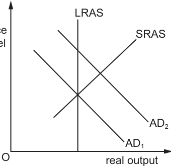
How can the subsequent impact on short-run and long-run macroeconomic equilibrium positions be shown using expectations-augmented Phillips curves?
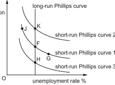
Options
A F to G to H
B F to G to K
C F to J to H
D F to J to K
Reasoning
- The initial long-run equilibrium occurs where AD1 intersects SRAS and LRAS in the AD/AS diagram, corresponding to point F on the Phillips curve. Point F lies on both the long-run Phillips curve (LRPC) and short-run Phillips curve 1 (SRPC1), representing the natural rate of unemployment where expected inflation equals actual inflation.
- When AD increases from AD1 to AD2, in the short run actual inflation rises above expected inflation. Firms increase output and employment to meet higher demand, so unemployment falls below the natural rate. This is a movement left along the existing SRPC1 to point J, which has lower unemployment and higher inflation than F.
- In the long run, workers and firms revise their inflation expectations upwards to match the higher actual inflation. This shifts the short-run Phillips curve up to SRPC2, and the economy returns to the natural rate of unemployment on the LRPC at point K, which has higher inflation than the initial equilibrium.
- The full adjustment path is F to J to K.
Answer
D
D
Background Concept
The expectations-augmented Phillips curve models the short-run and long-run relationship between inflation and unemployment. In the short run, if actual inflation is higher than the inflation rate workers and firms expected when they set wages and prices, real wages fall, so firms hire more workers and increase output. This lowers unemployment but raises inflation, shown as a movement along a given short-run Phillips curve (SRPC). In the long run, inflation expectations adjust to match actual inflation: workers demand higher nominal wages to restore their real wages, and firms raise their expected inflation for future pricing. This shifts the SRPC upwards (or downwards if inflation falls), and the economy returns to the natural rate of unemployment at the vertical long-run Phillips curve (LRPC).
The AD/AS model explains how aggregate demand shocks affect output and prices in the short and long run. An increase in AD raises the price level and real output in the short run, as the economy moves along the upward-sloping short-run aggregate supply curve (SRAS). In the long run, as nominal wages and input prices adjust to the higher price level, SRAS shifts left, returning output to the long-run aggregate supply (LRAS) level (potential output) at an even higher price level.
Understanding the Question
This 1-mark multiple-choice question asks you to identify the correct path of short-run and long-run macroeconomic equilibrium on an expectations-augmented Phillips curve, following an increase in aggregate demand from AD1 to AD2 shown in the accompanying AD/AS diagram. You need to link the effects of the AD shift to the corresponding movements and shifts on the Phillips curve, and match the full adjustment path to the labelled points F, G, H, J, K in the options.
Approach
To solve this, work through the adjustment in two stages, matching each stage to the Phillips curve diagram:
- First, confirm the initial long-run equilibrium: this is the point where AD1, SRAS and LRAS intersect in the AD/AS model, which corresponds to point F on the Phillips curve (on both SRPC1 and the LRPC, so unemployment is at the natural rate, and expected inflation equals actual inflation).
- Trace the short-run effect of the AD increase: in the short run, expectations are fixed, so the effect is a movement along the existing SRPC, not a shift of the curve. Higher AD raises output and employment, so unemployment falls below the natural rate, and inflation rises.
- Trace the long-run adjustment: as inflation expectations rise, the SRPC shifts up, and the economy returns to the natural rate of unemployment at a higher inflation rate, on the new SRPC.
You can also eliminate incorrect options early: any path that does not end on the LRPC (the vertical line) is wrong, because long-run equilibrium must be at the natural rate of unemployment. Any path that starts with a movement to the right of F (higher unemployment) is wrong, because an AD increase lowers unemployment in the short run.
Step-by-Step Reasoning
First, verify the initial equilibrium: Point F is the only point that lies on both the LRPC and SRPC1, so it is the initial long-run equilibrium, matching the AD/AS equilibrium where AD1 meets SRAS and LRAS. At this point, unemployment is at the natural rate, and expected inflation equals actual inflation.
Next, the short-run effect of AD shifting right from AD1 to AD2: In the short run, nominal wages and other input costs are fixed by existing contracts, so firms face higher demand for their output. They raise prices, increasing their revenue, and hire more workers to increase production. This reduces unemployment below the natural rate, while actual inflation rises above the previously expected inflation rate. On the Phillips curve, this is a movement along the existing SRPC1, because expected inflation has not yet changed. Lower unemployment corresponds to a position further left on the horizontal axis, and higher inflation to a higher position on the vertical axis: this is point J, which is to the left of F on SRPC1.
Then, the long-run adjustment: Over time, workers notice that the higher prices have reduced their real wages, so they negotiate higher nominal wages for future contracts. Firms also revise their expectations of future inflation upwards, as they have experienced higher inflation than they anticipated. This increase in expected inflation shifts the short-run Phillips curve upwards to SRPC2: for any given unemployment rate, workers will now demand higher nominal wages, and firms will expect higher input costs, so the inflation rate associated with any unemployment level is higher. In the AD/AS model, this higher wage cost shifts SRAS left, returning output to the LRAS level, so unemployment rises back to the natural rate. On the Phillips curve, this means the economy moves back to the LRPC at point K, which is on SRPC2, has the same unemployment rate as F, but a higher inflation rate.
Now evaluate the four options:
- Option A (F to G to H): Point G is to the right of F on SRPC1, meaning higher unemployment and lower inflation, which is the effect of a decrease in AD, not an increase. Point H is on SRPC3, which is below SRPC1, implying lower expected inflation, which is inconsistent with an AD increase. Incorrect.
- Option B (F to G to K): The first move to G is to higher unemployment, which does not match the short-run effect of an AD increase. Incorrect.
- Option C (F to J to H): The first move to J is correct for the short run, but H is on SRPC3, which is a lower SRPC implying lower expected inflation. An AD increase raises actual inflation, so expected inflation should rise, shifting the SRPC up, not down. Incorrect.
- Option D (F to J to K): This matches the full adjustment path: short-run movement left along SRPC1 to J (lower unemployment, higher inflation), then long-run shift up to SRPC2 and back to the LRPC at K (natural unemployment, higher inflation). Correct.
Key Takeaways
- The short-run effect of a positive AD shock is a movement along the existing SRPC to lower unemployment and higher inflation, as actual inflation exceeds expected inflation.
- The long-run effect of a demand shock is a shift of the SRPC, as inflation expectations adjust, and the economy returns to the natural rate of unemployment at the LRPC.
- The LRPC is vertical at the natural rate of unemployment, so all long-run equilibrium points must lie on this curve.
- An increase in AD shifts the SRPC upwards in the long run, as higher actual inflation leads to higher expected inflation.
Common Mistakes
- Confusing a movement along the SRPC with a shift of the SRPC: The short-run effect of an AD shock is always a movement along the existing SRPC, because inflation expectations are fixed in the short run. Only the long-run adjustment involves a shift of the SRPC.
- Reversing the direction of the short-run movement: Some students incorrectly assume that higher AD leads to higher unemployment, but in the short run, higher demand raises output and employment, so unemployment falls, meaning the movement is left along the SRPC (lower unemployment, higher inflation).
- Ignoring the long-run return to the natural rate of unemployment: Any option that ends at a point not on the LRPC (such as G or H) is incorrect, because in the long run, unemployment always returns to the natural rate, regardless of the inflation rate.
- Mixing up the direction of the SRPC shift: Higher expected inflation shifts the SRPC upwards (to SRPC2), not downwards, so a path ending on SRPC3 (like option C) is wrong.
Things to Be Careful About
- Always check that long-run equilibrium points lie on the vertical LRPC: this is a quick way to eliminate incorrect options, as only points K and F are on the LRPC.
- Distinguish clearly between the short run (fixed expectations, movement along SRPC) and long run (adjusted expectations, shift of SRPC): this is the core distinction in the expectations-augmented Phillips curve model.
- Match the direction of the AD shift to the Phillips curve path: an increase in AD always leads to lower unemployment in the short run, so the first step from the initial point F must be a move to the left (lower unemployment) along SRPC1, which eliminates options A and B immediately.
- Ensure you read the Phillips curve axes correctly: the vertical axis is inflation %, horizontal is unemployment %, so left is lower unemployment, higher is higher inflation; up is higher inflation, down is lower inflation.
How could high interest rates increase a country’s rate of inflation?
Options
A by increasing the current borrowing costs of business
B by increasing the current borrowing costs of government
C by increasing the foreign exchange rate of the currency
D by increasing the opportunity cost of spending
Answer
Higher interest rates increase firms' borrowing costs. Firms may pass on these higher costs to consumers by raising prices, which directly increases the rate of inflation. This is a cost-push effect.
Answer
A
A
Background Concept
Monetary policy affects inflation through several channels. The standard textbook channel is the demand-side channel: higher interest rates reduce consumption and investment, lowering aggregate demand (AD) and pulling inflation down. However, there is also a cost-push channel: higher interest rates raise the cost of borrowing for firms, which may increase their average costs of production. If firms have market power, they may pass these higher costs on to consumers in the form of higher prices, which directly increases the rate of inflation.
Understanding the Question
The question asks: "How could high interest rates increase a country's rate of inflation?" The key word is "increase" — the candidate must identify a mechanism through which higher interest rates cause inflation to rise, not fall. The four options present different potential channels. The correct answer is the one that describes a genuine cost-push mechanism.
Approach
Evaluate each option in turn:
- Option A: Higher interest rates increase firms' borrowing costs. This is a cost increase. If firms pass this on, prices rise -> inflation increases. This is the cost-push channel.
- Option B: Higher interest rates increase government borrowing costs. This is a cost to the government, not directly to firms. It does not directly raise consumer prices. It could lead to higher taxes or lower spending, which would reduce AD and lower inflation.
- Option C: Higher interest rates can attract foreign capital, causing the currency to appreciate (increase in the foreign exchange rate). An appreciation makes imports cheaper, which reduces import prices and lowers inflation. This is a disinflationary channel, not an inflationary one.
- Option D: Higher interest rates increase the opportunity cost of spending (saving becomes more attractive). This reduces consumption, lowers AD, and reduces inflation. This is the standard demand-side channel.
Only Option A describes a mechanism that could increase inflation.
Step-by-Step Reasoning
- Identify the effect of higher interest rates on firms: Higher interest rates increase the cost of borrowing for firms. This includes the cost of working capital loans, investment loans, and overdrafts.
- Trace the effect on firms' costs: These higher borrowing costs are a component of firms' total costs. They raise average total cost (ATC) and marginal cost (MC).
- Trace the effect on prices: Firms, especially those with some market power (which is most firms in the real world), may respond to higher costs by raising their prices to maintain profit margins. This is a classic cost-push inflation mechanism.
- Conclude: If firms raise prices, the general price level rises, increasing the rate of inflation.
Key Takeaways
- Monetary policy has multiple transmission channels. The most familiar is the demand-side channel (higher rates -> lower AD -> lower inflation). But there is also a cost-push channel (higher rates -> higher costs -> higher prices).
- The question tests the ability to distinguish between these channels and to identify which one could produce an increase in inflation.
- Always consider both demand-side and supply-side effects when analysing the impact of a policy change.
Common Mistakes
- Choosing Option D: This is the most common mistake. Candidates know that higher interest rates reduce spending, so they assume this must reduce inflation. They forget that the question asks for a mechanism that increases inflation.
- Choosing Option C: Candidates may think that higher interest rates attract foreign capital, which increases demand for the currency, which could increase the price of imports (if the currency depreciates). But the option says "increasing the foreign exchange rate" which means an appreciation (the currency becomes stronger). An appreciation reduces import prices and lowers inflation.
- Confusing cost-push and demand-pull: The cost-push channel is less commonly taught, so candidates may not recognise it.
Things to Be Careful About
- Read the question carefully: "increase a country's rate of inflation" — the answer must describe a mechanism that raises inflation, not lowers it.
- Understand the direction of the exchange rate effect: "increasing the foreign exchange rate" means the currency appreciates (buys more foreign currency), which is disinflationary.
- Distinguish between the effect on firms (Option A) and the effect on the government (Option B). The government's borrowing costs do not directly feed into consumer prices in the same way.
What is most likely to influence subsequent increases in national income as a result of a government policy of reduced interest rates?
Options
A marginal cost
B marginal efficiency of capital
C marginal product
D marginal utility
Reasoning
A reduction in interest rates lowers the cost of borrowing, making more investment projects profitable if their expected rate of return exceeds the lower interest rate. The marginal efficiency of capital (MEC) is the expected rate of return on the last unit of capital. A fall in the interest rate increases the number of projects for which MEC exceeds the cost of funds, so planned investment rises. Through the multiplier, this rise in investment increases aggregate demand and hence national income.
Answer
B
B
Background Concept
Marginal efficiency of capital (MEC) is the expected rate of return on an additional unit of capital, calculated by discounting the expected stream of future profits from that capital and expressing it as a percentage of its cost. Firms compare the MEC of a potential investment project with the prevailing interest rate (which represents the cost of borrowing or the opportunity cost of using own funds). If MEC > interest rate, the project is profitable and should be undertaken; if MEC < interest rate, it should not. A reduction in the interest rate therefore shifts the threshold, making more projects viable, which increases planned investment spending. The rise in investment then, through the multiplier process, causes a larger increase in national income.
The other options are marginal concepts from microeconomics that do not directly mediate the link between interest rates and national income:
- Marginal cost (A) – the additional cost of producing one more unit of output; it guides a firm's output decision, not its investment decision.
- Marginal product (C) – the extra output from one more unit of a variable input; it informs hiring and production decisions in the short run, not investment in new capital.
- Marginal utility (D) – the extra satisfaction from consuming one more unit; it governs consumer choice, not firms' investment behaviour.
Understanding the Question
The question asks: given a government policy that reduces interest rates, which marginal concept is most likely to influence the subsequent increases in national income? The chain is: lower interest rates → cheaper borrowing → more investment → multiplier effect → higher national income. The key link is the criterion firms use to decide whether to invest. That criterion is the marginal efficiency of capital. The question tests whether you can pick the one marginal concept that is directly relevant to the investment decision in macroeconomics, rather than confusing it with other marginal concepts from microeconomics.
Approach
- Identify the economic mechanism: a cut in interest rates stimulates aggregate demand primarily through investment (and possibly consumption of durables).
- Recall what firms compare to the interest rate when deciding whether to invest: the expected rate of return on capital, i.e. the marginal efficiency of capital.
- Recognise that the multiplier magnifies any rise in investment into a larger increase in national income.
- Eliminate the three distractors by noting that they relate to short-run production decisions (marginal cost, marginal product) or consumer choice (marginal utility) and do not directly connect interest rates to investment and income.
Step-by-Step Reasoning
-
Identify the policy and its direct effect: A reduction in interest rates by the government (or monetary authority) lowers the cost of borrowing for firms and households. It also reduces the opportunity cost of using retained profits for investment because the return on alternative financial assets falls.
-
Link to investment: Firms undertake investment projects if the expected return exceeds the cost of finance. The expected return on the last unit of capital is the marginal efficiency of capital (MEC). When interest rates fall, some projects that were previously unprofitable (MEC < old interest rate) become profitable (MEC > new interest rate). So planned investment rises.
-
Link to national income: An increase in investment is a component of aggregate demand (I). The multiplier then amplifies this initial rise: the extra spending becomes income for others, who spend a fraction of it, leading to further rounds of spending and income. Thus national income rises by a multiple of the initial increase in investment.
-
Why the other options are wrong:
- Marginal cost (A): A firm considers marginal cost when deciding how much to produce given its existing capital stock. A change in interest rates does not directly affect marginal cost; it affects the cost of new capital, not the cost of producing more output from existing plant.
- Marginal product (C): Marginal product of labour or capital informs short-run hiring or production decisions, but the decision to add new capital (investment) weighs the expected return from that capital (MEC) against the cost of funds (interest rate).
- Marginal utility (D): This is a consumer concept. While lower interest rates may also boost consumption (especially of durable goods financed by credit), the direct and dominant channel to national income is through investment, and the relevant marginal concept for investment is the MEC.
Key Takeaways
- The marginal efficiency of capital is the critical link between interest rates and investment.
- Investment decisions are made by comparing MEC with the interest rate.
- Through the multiplier, changes in investment cause larger changes in national income.
- Do not confuse investment criteria (MEC) with short-run production or consumption concepts.
Common Mistakes
- Picking marginal cost because of a vague association of “cost” with “interest rate” – but marginal cost is about the cost of producing current output, not the cost of financing new capital.
- Picking marginal product because it sounds like“marginal product of capital” – but that is a short-run concept; the investment decision depends on expected returns, not current physical output per unit.
- Picking marginal utility because lower interest rates can affect consumption – but the question explicitly asks about increases in national income via a government policy of reduced interest rates, and the most likely channel is investment, where the MEC is the decisive factor.
Things to Be Careful About
- Read marginal concepts carefully: each one belongs to a specific economic decision (production, hiring, consumption, investment).
- Remember the chain: interest rate → MEC comparison → investment → multiplier → national income.
- Do not overthink – the MCQ is testing a specific, standard linkage from the syllabus.
Which policy to reduce a current account deficit on the balance of payments could be described as an expenditure-switching policy?
Options
A a decrease in government spending
B a decrease in the exchange rate of the country’s currency
C an increase in domestic income taxes
D an increase in domestic interest rates
Answer
An expenditure-switching policy aims to shift domestic and foreign spending away from imports and towards domestically produced goods and services, without directly changing the level of aggregate demand. A decrease in the exchange rate (a depreciation or devaluation) makes exports cheaper in foreign currency and imports dearer in domestic currency, thereby switching expenditure towards domestic output. Options A, C and D are all expenditure-reducing policies: they lower aggregate demand and thus reduce the demand for imports, but they do not switch expenditure.
Answer
B
B
Background Concept
The balance of payments current account records a country's trade in goods and services, investment income, and transfers. A current account deficit means the value of imports exceeds the value of exports. Policies to correct a deficit are classified into two broad types:
-
Expenditure-switching policies: These aim to change the composition of spending between domestic and foreign goods, without necessarily changing the total level of spending. The main examples are exchange rate changes (depreciation/devaluation) and trade protection (tariffs, quotas, subsidies to domestic producers).
-
Expenditure-reducing policies: These aim to reduce the total level of aggregate demand in the economy, which in turn reduces the demand for imports. Examples include contractionary fiscal policy (higher taxes, lower government spending) and contractionary monetary policy (higher interest rates).
Understanding the Question
The question asks which of the four listed policies is an expenditure-switching policy. The key is to recall the definition and identify which policy directly alters relative prices between domestic and foreign goods, rather than simply reducing total spending.
Approach
- Recall the definition of expenditure-switching policy.
- Evaluate each option against that definition.
- Identify the correct option.
Step-by-Step Reasoning
-
Option A: a decrease in government spending – This is a contractionary fiscal policy. It reduces aggregate demand, which will reduce the demand for imports, but it does not switch expenditure towards domestic goods. It is an expenditure-reducing policy.
-
Option B: a decrease in the exchange rate of the country’s currency – A depreciation (or devaluation under a fixed system) makes exports cheaper for foreign buyers and imports more expensive for domestic consumers. This directly switches spending from foreign goods to domestic goods. It is the classic example of an expenditure-switching policy.
-
Option C: an increase in domestic income taxes – This reduces disposable income, lowering consumption and aggregate demand. It reduces imports but does not switch expenditure. It is expenditure-reducing.
-
Option D: an increase in domestic interest rates – This is contractionary monetary policy. Higher interest rates reduce investment and consumption, lowering aggregate demand and imports. It is expenditure-reducing.
Therefore, only option B fits the definition.
Key Takeaways
- Expenditure-switching policies change relative prices between domestic and foreign goods.
- Expenditure-reducing policies lower aggregate demand.
- Exchange rate changes are the primary expenditure-switching tool.
Common Mistakes
- Confusing expenditure-switching with expenditure-reducing policies.
- Thinking that any policy that reduces imports is automatically expenditure-switching.
Things to Be Careful About
- The question asks for the policy that could be described as expenditure-switching. Only one option fits.
- Note that a decrease in the exchange rate is a depreciation (or devaluation), which is the classic example.
Which components are included in the financial account of the balance of payments?
Options
| foreign direct investment | interest, profits and dividends | |
|---|---|---|
| A | included | not included |
| B | not included | not included |
| C | included | included |
| D | not included | included |
Answer
The financial account records transactions in financial assets and liabilities, including foreign direct investment (FDI), portfolio investment, and reserve assets. Interest, profits, and dividends are recorded in the current account as primary income, not in the financial account. Therefore, FDI is included, and interest, profits, and dividends are not included. Option A is correct.
A
Background Concept
The balance of payments (BoP) is a record of all economic transactions between residents of one country and the rest of the world over a period. It has three main accounts: the current account, the capital account, and the financial account.
- Current Account: Records trade in goods and services, primary income (such as interest, profits, and dividends from investments), and secondary income (transfers).
- Capital Account: Records capital transfers and acquisition/disposal of non-produced, non-financial assets.
- Financial Account: Records transactions in financial assets and liabilities, such as foreign direct investment (FDI), portfolio investment (e.g., shares and bonds), financial derivatives, and reserve assets.
Foreign direct investment (FDI) involves a lasting interest in a foreign enterprise, typically with ownership of 10% or more. It is a financial transaction and thus appears in the financial account. Interest, profits, and dividends are returns on investments and are classified as primary income in the current account.
Understanding the Question
This question asks which of two items – foreign direct investment and interest, profits, and dividends – are included in the financial account of the balance of payments. The answer is based solely on the standard classification used in international economics. The options present combinations of inclusion (yes/no) for each item.
Approach
Recall the standard components of the financial account. Compare each item against the definition: financial account entries involve changes in ownership of financial assets and liabilities. FDI clearly qualifies. Interest, profits, and dividends are income flows, not asset transactions, so they belong in the current account. Therefore, the correct combination is FDI included, interest payments not included.
Step-by-Step Reasoning
-
Foreign direct investment (FDI): FDI involves acquiring a controlling stake in a foreign enterprise or setting up new operations abroad. It is a cross-border investment where the investor intends to exert significant influence. This is a transaction in financial assets, so it is recorded in the financial account. The BoP convention places FDI under the financial account (often as 'direct investment'). Therefore, FDI is included.
-
Interest, profits, and dividends: These are earnings from prior investments. For example, if a UK resident owns shares in a US company, dividends paid are income for the UK resident. Such earnings are considered primary income and are recorded in the current account, not the financial account. The financial account records the initial purchase or sale of the asset, not the subsequent income flows. Therefore, interest, profits, and dividends are not included in the financial account.
-
Matching to options:
- Option A: FDI included, interest, profits, and dividends not included – matches our analysis.
- Option B: both not included – incorrect because FDI is included.
- Option C: both included – incorrect because interest, profits, and dividends are not included.
- Option D: FDI not included, interest, profits, and dividends included – incorrect.
Thus, A is correct.
Key Takeaways
- The financial account records international transactions in financial assets (e.g., FDI, portfolio equity, debt securities).
- The current account records income flows such as interest, profits, and dividends (primary income).
- Knowing the distinction between stocks (financial account) and flows (current account income) is essential for balance of payments questions.
Common Mistakes
- Confusing income flows with financial transactions: Many students incorrectly place interest and dividends in the financial account because they associate them with investment. But the financial account records the investment itself (the asset), not the return on it.
- Treating 'capital account' and 'financial account' as the same. Under the IMF BPM6 format, the capital account is small (transfers, debt forgiveness); the old 'capital account' was split into the current and financial accounts. This question uses the modern three-account presentation.
Things to Be Careful About
- Remember the exact terminology: 'financial account' is the modern term; older textbooks may use 'capital account' differently. Always check the syllabus.
- Note that certain exceptional items like reinvested earnings can be recorded in both the current account (as income) and the financial account (as FDI) – but that is an advanced nuance not tested here. For standard multiple-choice, interest, profits, and dividends are current account items.
It is often argued that the UN Human Development Index (HDI) is a better indicator of economic development than income per capita because it adjusts for
Options
A average hours worked by the population.
B environmental pollution.
C inequality in income distribution.
D life expectancy at birth.
Answer
The Human Development Index (HDI) is a composite indicator that combines three dimensions: life expectancy at birth (health), education (expected and mean years of schooling), and GNI per capita (income). Income per capita captures only the income dimension. Therefore, HDI adjusts for life expectancy at birth, which is not reflected in income per capita alone.
Option D is correct.
D
Background Concept
The Human Development Index (HDI), published by the United Nations, was designed to provide a more comprehensive measure of economic development than simple income per capita. It is based on the idea that development should be measured by people's capabilities and opportunities, not just by the amount of money they earn. The HDI consists of three dimensions:
- Health: measured by life expectancy at birth.
- Education: measured by expected years of schooling (for children) and mean years of schooling (for adults).
- Standard of living: measured by GNI per capita (adjusted for purchasing power parity).
Income per capita alone (such as GDP or GNI per capita) only captures the third dimension, ignoring differences in health and education. Therefore, HDI is said to 'adjust' for these non-income aspects, giving a fuller picture of well-being.
Understanding the Question
The question asks: 'It is often argued that the UN Human Development Index (HDI) is a better indicator of economic development than income per capita because it adjusts for ____'. The candidate must identify which of the listed factors is actually a component of the HDI that income per capita misses.
- Option A: average hours worked – not part of HDI.
- Option B: environmental pollution – not directly included in HDI (there is a separate Planetary Pressures-adjusted HDI, but the standard HDI does not include it).
- Option C: inequality in income distribution – the standard HDI does not adjust for inequality (though there is an Inequality-adjusted HDI, IHDI, but the question specifically refers to the standard HDI).
- Option D: life expectancy at birth – correctly a component of HDI.
Thus D is the correct answer.
Approach
To answer this multiple-choice question, recall the exact components of the HDI. Compare each option against those components. The three components are life expectancy, education, and income. The only option that matches one of these is D. The others are plausible distractors but are not part of the standard HDI.
Step-by-Step Reasoning
- Recall the standard HDI consists of three dimensions:
- Life expectancy at birth (health)
- Expected years of schooling and mean years of schooling (education)
- GNI per capita (income/standard of living)
- Income per capita covers only the third dimension. So the 'adjustment' that HDI makes is to add the first two dimensions.
- Evaluate each option:
- A (average hours worked): This is not a component of HDI. Hours worked may relate to labour market conditions but are not used in the HDI calculation.
- B (environmental pollution): While pollution affects well-being, the standard HDI does not include an environmental dimension. (The UN has developed an experimental 'green' HDI, but the question refers to the standard HDI.)
- C (inequality in income distribution): The standard HDI uses average GNI per capita and does not directly incorporate inequality. The Inequality-adjusted HDI (IHDI) does, but that is a separate indicator; the question says 'the UN Human Development Index (HDI)', which is the standard version.
- D (life expectancy at birth): This is the health dimension of HDI. Income per capita does not capture health outcomes, so HDI provides a broader measure by including life expectancy.
- Therefore, the correct answer is D.
Key Takeaways
- The HDI is a composite indicator that goes beyond income to include health (life expectancy) and education.
- A key exam skill is to know the exact composition of commonly used composite indicators such as HDI.
- Do not confuse the standard HDI with its variants (IHDI, Green HDI) unless the question specifically references them.
Common Mistakes
- Choosing 'inequality in income distribution' (C) because some students think HDI adjusts for inequality. The standard HDI does not; that is the Inequality-adjusted HDI (IHDI).
- Choosing 'environmental pollution' (B) because students associate 'development' with environmental concerns. The standard HDI does not include pollution.
- Choosing 'average hours worked' (A) due to confusion with other measures like the Human Poverty Index or the Gender Development Index.
Things to Be Careful About
- Always learn the precise components of the HDI: life expectancy, education (schooling), and income.
- In multiple-choice questions, the presence of a 'distractor' that is a variant of the correct concept (e.g., inequality-adjusted HDI) is common. Read the question wording carefully – it says 'the UN Human Development Index (HDI)', not 'the Inequality-adjusted HDI'.
- Know that income per capita is a monetary measure; HDI adds non-monetary dimensions.
Some conditions for providing foreign aid to low-income countries can be restrictive.
Which kind of aid fits this description?
Options
A food aid in the event of natural catastrophes such as severe drought
B grants that are tied to purchasing donor country goods
C loans that are repaid over a long period at a low rate of interest
D technical assistance using highly skilled worker transfers to provide support
Reasoning
Foreign aid that is tied to purchasing goods from the donor country imposes restrictions on the recipient: the aid cannot be used to buy from the cheapest source or to support local industries. This makes it restrictive. In contrast, food aid in catastrophes (A) is emergency, unconditional; concessional loans (C) are financial assistance with favourable terms but no purchasing restriction; technical assistance (D) is transfer of expertise, not restrictive. Therefore, option B correctly fits the description.
Answer
B
B
Background Concept
Foreign aid can be provided in various forms: grants, loans, technical assistance, food aid, etc. A key distinction is between tied and untied aid. Tied aid requires the recipient to spend the aid money on goods and services from the donor country, often at higher prices than available elsewhere. This condition restricts the recipient's freedom to use the aid for its most efficient purpose. Untied aid has no such restriction, allowing the recipient to purchase from the cheapest source or to use the funds flexibly. Other forms like concessional loans have repayment conditions but are not typically considered restrictive in the same way; technical assistance involves transferring skills and knowledge, which may come with conditions but not usually on purchasing.
Understanding the Question
The question asks: "Some conditions for providing foreign aid to low-income countries can be restrictive. Which kind of aid fits this description?" The key word is "restrictive" – it implies that the aid comes with conditions that limit the recipient's freedom to choose how to use the aid. The four options represent different types of aid. We need to identify the one that is most clearly associated with restrictive conditions, specifically tied aid.
Approach
Evaluate each option against the definition of restrictive conditions:
- Option A: food aid in natural catastrophes – this is emergency aid, typically unconditional and provided without restrictive purchasing requirements.
- Option B: grants tied to purchasing donor country goods – this is the classic definition of tied aid, which is explicitly restrictive.
- Option C: loans repaid over a long period at low interest – these are concessional loans; they have repayment conditions but not restrictive in the sense of limiting how the funds are spent (the loan itself is financial aid, and the repayment terms are favourable, not restrictive).
- Option D: technical assistance using skilled worker transfers – this is a form of capacity building; it may have conditions on cooperation but not restrictive purchasing requirements.
Thus, only option B fits the description of having restrictive conditions attached to the aid.
Step-by-Step Reasoning
-
Read the question carefully: "Some conditions for providing foreign aid to low-income countries can be restrictive." The phrase "can be restrictive" indicates that the aid type itself is associated with restrictive conditions.
-
Analyse each option:
- Option A: food aid in the event of natural catastrophes such as severe drought. This is emergency humanitarian aid. It is usually provided without conditions about where the food is purchased (though sometimes it may be tied, but in general it is not considered restrictive; the context is emergency relief). The question does not specify that it is tied, so it is not the best fit.
- Option B: grants that are tied to purchasing donor country goods. This is explicitly tied aid. The condition is that the recipient must use the grant money to buy goods from the donor country. This restricts the recipient's ability to buy from cheaper or more efficient sources, imposes a condition on the use of the aid, and is widely recognised as a restrictive practice.
- Option C: loans that are repaid over a long period at a low rate of interest. This describes a concessional loan. The terms are favourable, but the condition is about repayment, not about how the loan proceeds are spent. The loan itself is not restrictive in the sense of the question; the recipient can use the funds for any agreed purpose. The condition is not restrictive relative to the aid's use.
- Option D: technical assistance using highly skilled worker transfers to provide support. This involves sending experts to help build capacity. The condition is not about purchasing; it is about receiving expertise. While there may be conditions on cooperation, it is not typically considered restrictive in the same way as tied aid.
-
Conclusion: The only option that clearly involves a restrictive condition (the condition to purchase from the donor) is option B. Therefore, the correct answer is B.
Key Takeaways
- Tied aid is a form of foreign aid that requires the recipient to spend the aid on goods and services from the donor country, making it restrictive.
- Other forms of aid (emergency aid, concessional loans, technical assistance) are generally not considered restrictive in the same sense.
- Understanding the different types of aid and their conditions is important for evaluating the effectiveness and fairness of aid policies.
Common Mistakes
- Confusing concessional loans with tied aid: both are forms of aid, but the condition in tied aid is about purchasing, not about repayment.
- Thinking that any condition makes aid restrictive: the question specifically asks for aid that fits the description of having restrictive conditions, and tied aid is the classic example.
- Overlooking the phrase "tied to purchasing donor country goods" as the key restrictive condition.
Things to Be Careful About
- The question is about the nature of the condition, not the type of aid itself. Tied aid is explicitly restrictive because it imposes a condition on the use of the funds.
- The other options may have implicit conditions (e.g., loans must be repaid, technical assistance requires cooperation), but they are not the type of restrictive conditions that the question highlights.
- The mark scheme confirms that option B is correct.
What is most likely to cause the living standards of a country to rise?
Options
A an increase in the number of doctors
B an increase in the gold reserves
C an increase in the number of people per house
D an increase in the money supply
Reasoning
Living standards refer to the material and non-material well-being of a country's population. An increase in the number of doctors directly improves access to healthcare, which is a key non-monetary indicator of living standards (e.g., the HDI includes health indicators). This raises the quality and availability of medical services, reducing mortality and morbidity, and thus enhancing welfare.
An increase in gold reserves (B) does not directly affect the population's access to goods and services. An increase in people per house (C) implies overcrowding and lower housing quality, which reduces living standards. An increase in the money supply (D) may cause inflation if not matched by output, eroding real purchasing power and potentially harming living standards.
Answer
A
A
Background Concept
Living standards are a measure of the quality of life enjoyed by the population of a country. They are assessed using both monetary indicators (such as real GDP per capita, GNI per capita, and purchasing power parity) and non-monetary indicators (such as life expectancy, literacy rates, access to clean water, healthcare provision, and housing quality). Composite indices like the Human Development Index (HDI) combine income, health, and education to give a broader picture. An improvement in living standards means that, on average, people are better off in terms of their material consumption, health, education, and overall well-being.
Understanding the Question
This is a multiple-choice question asking which of four changes is most likely to cause a rise in a country's living standards. The options are:
- A: an increase in the number of doctors
- B: an increase in the gold reserves
- C: an increase in the number of people per house
- D: an increase in the money supply
The question tests the ability to distinguish between factors that directly enhance human welfare and those that are either irrelevant or harmful. The correct answer is the one that most directly and unambiguously improves a key dimension of living standards.
Approach
Evaluate each option in turn against the definition of living standards. For each, ask: does this change directly improve the health, education, income, or overall well-being of the population? If not, it is unlikely to raise living standards. The option that most clearly passes this test is the correct answer.
Step-by-Step Reasoning
-
Option A: an increase in the number of doctors. More doctors mean better access to healthcare services. This can lead to lower infant mortality, higher life expectancy, and improved treatment of diseases. Healthcare is a fundamental component of non-monetary living standards and is included in the HDI. Therefore, this option directly and positively affects living standards.
-
Option B: an increase in the gold reserves. Gold reserves are a store of value and part of a country's wealth, but they do not directly translate into improved living standards unless they are used to finance imports of goods and services that benefit the population. In themselves, gold reserves sitting in a vault do not provide healthcare, education, or consumption goods. They are not a direct determinant of living standards.
-
Option C: an increase in the number of people per house. This indicates overcrowding, which is associated with poorer housing quality, increased stress, higher risk of disease transmission, and lower overall well-being. This change would reduce, not raise, living standards.
-
Option D: an increase in the money supply. An increase in the money supply, if not accompanied by a corresponding increase in real output, is likely to cause demand-pull inflation. Inflation erodes the purchasing power of money, reducing real incomes and potentially harming living standards, especially for those on fixed incomes. It does not directly improve welfare.
Thus, only option A represents a clear and direct improvement in living standards.
Key Takeaways
- Living standards are multi-dimensional and include both monetary and non-monetary factors.
- Healthcare provision (e.g., number of doctors) is a key non-monetary indicator.
- Not all increases in national wealth (e.g., gold reserves) automatically improve living standards; the wealth must be used to benefit the population.
- Overcrowding and inflation are generally detrimental to living standards.
Common Mistakes
- Choosing B (gold reserves) because it seems like 'wealth' — but wealth that is not used for consumption or investment in human welfare does not raise living standards.
- Confusing an increase in the money supply with an increase in real income — the former can cause inflation and reduce real purchasing power.
- Misinterpreting 'people per house' as a sign of economic growth rather than overcrowding.
Things to Be Careful About
- Always link the change to the actual well-being of the population, not just to a macroeconomic aggregate.
- Remember that non-monetary indicators (health, education, housing) are as important as income in measuring living standards.
Globalisation means that goods and services, capital and labour are traded on a worldwide basis.
Which combination illustrates that each trade partner can benefit when a low-income country trades with a high-income country?
Options
| the low-income country | the high-income country | |
|---|---|---|
| A | contracts are not always fulfilled due to corrupt practices | agrees to increase investment in the infrastructure of low-income countries |
| B | experiences liquidity problems that restrict investment | transfers short-term government loans repayable at high interest rates |
| C | multinational companies repatriate profits from mining of rare minerals for export | receives supplies at high prices from multinationals to meet excess demands for rare metals |
| D | supplies seasonal labour to overcome shortages for picking fruit crops | repatriates wages to families of seasonal workers |
Answer
The question asks which combination illustrates mutual benefit for both trading partners. Option D shows the low-income country supplying seasonal labour to overcome shortages in the high-income country, while the high-income country repatriates wages to the families of the seasonal workers. This is a mutually beneficial exchange: the high-income country gains labour to meet demand, and the low-income country receives financial inflows (remittances) that can raise living standards and enable investment. Options A, B, and C involve negative outcomes (corruption, liquidity problems, profit repatriation) or one-sided benefits, so they do not illustrate mutual benefit. Therefore the correct answer is D.
D
Background Concept
Globalisation refers to the increasing integration of economies through the movement of goods, services, capital, and labour across borders. A key potential benefit of globalisation is that all participating countries can gain, provided the terms of trade and factor flows are mutually advantageous. For labour movements, a low-income country can export surplus labour and receive remittance payments, which boost national income and reduce unemployment. A high-income country can fill labour shortages (e.g., seasonal agricultural work) at lower cost than domestic alternatives, increasing output and controlling wage inflation.
Understanding the Question
The question presents four scenarios of trade between a low-income country and a high-income country. You must identify which combination (one action/outcome for each country) shows that both parties benefit. The key phrase is "each trade partner can benefit". The options mix positive and negative descriptions. Only one option shows gains on both sides; the others involve exploitation, costs, or one-sided advantages.
Approach
Read each option carefully. For each, ask: does the low-income country gain? Does the high-income country gain? If one or both experience a net loss or a zero-sum transfer, discard it. The correct answer will show a positive outcome for each, reflecting the mutual gains from voluntary exchange. The extract defines globalisation as trade in goods, capital, and labour, so factor movements are included.
Step-by-Step Reasoning
- Option A: The low-income country suffers from corruption (contracts not fulfilled), which is a cost. The high-income country agrees to increase investment in infrastructure. The high-income country may gain from improved infrastructure (future returns), but the low-income country experiences a clear negative (corruption). Not mutual benefit.
- Option B: The low-income country experiences liquidity problems that restrict investment (a cost). The high-income country transfers short-term government loans at high interest rates. The high-income country gains interest income, but the low-income country faces a financial burden (high interest payments). Not mutual benefit.
- Option C: The low-income country suffers repatriation of profits by MNCs (loss of income). The high-income country receives supplies at high prices from those same MNCs (a cost). Both sides experience losses or inefficiencies. Not mutual benefit.
- Option D: The low-income country supplies seasonal labour (exports labour) and receives repatriated wages (remittances). The high-income country overcomes labour shortages (increases output, avoids bottlenecks). Both sides gain: the low-income country gets income; the high-income country gets needed labour. Thus mutual benefit is illustrated.
Key Takeaways
- Mutual gains from trade require voluntary exchange where each party values what they receive more than what they give up.
- Labour migration can be mutually beneficial: the source country gains remittances and reduced unemployment; the host country gains labour to meet demand.
- One-sided benefits or negative outcomes (corruption, debt burdens, profit repatriation without local benefit) do not illustrate mutual gain.
Common Mistakes
- Assuming that any trade is automatically mutually beneficial without checking each side's net outcome. For example, profit repatriation (option C) may benefit the MNC but not necessarily the low-income country.
- Not reading carefully: option A mentions "contracts not always fulfilled" which is a negative, but investment is positive; the combination is not fully positive.
- Overlooking that the question requires each partner to benefit, not just one or the combination to be neutral.
Things to Be Careful About
- An answer can be correct even if the benefit is indirect (labour supply for wages). The key is that both countries are better off in that transaction.
- Do not assume corruption or high interest rates are acceptable; they impose costs that outweigh any potential benefit.
- Focus on the specific combination given, not on what might happen in a broader context. The question explicitly gives the outcomes for each partner.
Your score so far
Answer a question to start scoring
Your marks add up here as you work through the paper.