Economics 9708/33 — May/June 2024
Cambridge A-Level · A Level Multiple Choice · answer key with instant marking and worked solutions
Topics Government Policies to Correct Market Failure · Externalities, Social Costs and Benefits · Objectives and Pricing Policies of Firms · Growth and Survival of Firms · Employment and Unemployment · Macroeconomic Objectives and Policy Conflicts · +17 more
Tap an option under each question to check it — your score builds as you go.
Which statement about the concept of utility is correct?
Options
A Diminishing marginal utility means that producers become less efficient the more they produce.
B If marginal utility is above average utility, average utility must be rising.
C The equi-marginal principle says that a consumer gets equal total satisfaction from each item purchased.
D Total utility continually rises as the level of consumption rises.
Reasoning
Marginal utility (MU) is the change in total utility from consuming one more unit. Average utility (AU) is total utility divided by quantity. Whenever a marginal value is above the average value, it pulls the average up. Therefore, if MU > AU, AU must be rising.
Option A is incorrect because diminishing marginal utility refers to the consumer's satisfaction, not the producer's efficiency. Option C is incorrect because the equi-marginal principle states that a consumer maximises utility when the marginal utility per dollar spent is equal across all goods, not that total satisfaction from each item is equal. Option D is incorrect because total utility can fall if marginal utility becomes negative (e.g., overconsumption).
Answer
B
B
Background Concept
Utility theory explains how consumers derive satisfaction from consuming goods and services. Two key concepts are:
- Total Utility (TU): The total satisfaction a consumer gets from consuming a certain quantity of a good.
- Marginal Utility (MU): The additional satisfaction gained from consuming one more unit of the good. MU = change in TU / change in quantity.
A fundamental observation is the law of diminishing marginal utility: as a consumer consumes more units of a good within a given time period, the additional satisfaction from each extra unit eventually falls. This is why demand curves slope downwards — consumers are only willing to pay a lower price for additional units.
The equi-marginal principle (also called the utility-maximising rule) states that a consumer with a fixed income will maximise total utility when the marginal utility per unit of currency spent is equal across all goods. In other words, MUx / Px = MUy / Py for all goods X and Y.
A useful mathematical relationship exists between marginal and average values (not just in utility, but in any context like cost or product): if the marginal value is above the average value, the average must be rising; if the marginal value is below the average, the average must be falling; if they are equal, the average is constant.
Understanding the Question
This is a multiple-choice question testing precise understanding of utility theory terminology and relationships. The question asks which of four statements about utility is correct. Each option presents a common misconception or a misstatement of a key concept. The correct answer requires knowing the relationship between marginal and average utility.
Approach
Evaluate each option systematically against the definitions:
- Option A: Check if diminishing marginal utility relates to producer efficiency or consumer satisfaction.
- Option B: Apply the marginal-average relationship to utility.
- Option C: Check the exact wording of the equi-marginal principle.
- Option D: Consider whether total utility can ever fall.
Step-by-Step Reasoning
Option A: "Diminishing marginal utility means that producers become less efficient the more they produce."
- Diminishing marginal utility is a concept from consumer theory, not producer theory. It describes how a consumer's additional satisfaction falls with more consumption. Producer efficiency is about costs and output, governed by the law of diminishing returns (a different concept). This option confuses two separate ideas. Therefore, A is incorrect.
Option B: "If marginal utility is above average utility, average utility must be rising."
- This is a mathematical truth. Average utility (AU) = TU / Q. Marginal utility (MU) is the addition to TU from the last unit. If the last unit adds more to TU than the current average (i.e., MU > AU), it pulls the average up. For example, if AU is 10 and the next unit gives MU of 15, the new AU becomes (old TU + 15) / (Q + 1), which will be higher than 10. This relationship holds for any marginal-average pair (e.g., marginal cost and average cost, marginal product and average product). Therefore, B is correct.
Option C: "The equi-marginal principle says that a consumer gets equal total satisfaction from each item purchased."
- The equi-marginal principle does not say total satisfaction from each item is equal. It says the consumer allocates spending so that the marginal utility per dollar is equal across all goods. This maximises total utility given the budget constraint. The total satisfaction from different items can be very different (e.g., a car vs. a chocolate bar). Therefore, C is incorrect.
Option D: "Total utility continually rises as the level of consumption rises."
- Total utility rises as long as marginal utility is positive. However, if consumption continues beyond the point of satiety, marginal utility can become negative (e.g., eating too much food causes discomfort). When MU is negative, each additional unit reduces total utility, so TU falls. Therefore, TU does not continually rise; it can peak and then decline. Therefore, D is incorrect.
Key Takeaways
- Understand the precise definitions of total utility, marginal utility, and the equi-marginal principle.
- The marginal-average relationship is a powerful analytical tool that applies across many economic contexts (utility, cost, product, revenue).
- Be careful not to confuse consumer theory concepts (utility) with producer theory concepts (returns, costs).
- Read each option carefully — examiners often test subtle distinctions in wording.
Common Mistakes
- Confusing diminishing marginal utility (consumer satisfaction) with diminishing returns (production efficiency).
- Misstating the equi-marginal principle as equal total satisfaction rather than equal marginal utility per dollar.
- Assuming total utility always increases with consumption, forgetting that negative marginal utility is possible.
- Not applying the marginal-average relationship correctly, even though it is a standard mathematical property.
Things to Be Careful About
- In multiple-choice questions, eliminate clearly wrong options first, then focus on the remaining contenders.
- For marginal-average questions, remember the rule: marginal above average pulls average up; marginal below average pulls average down.
- The equi-marginal principle is about optimisation at the margin, not about total values.
- Utility is subjective and cannot be measured cardinally in reality, but the model assumes it can be for analytical purposes.
The diagram shows indifference curves I1, I2 and a budget line T.
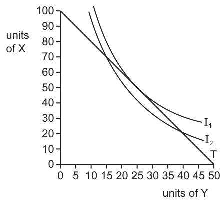
Which combination of X and Y gives the consumer maximum satisfaction?
Options
| units of X | units of Y | |
|---|---|---|
| A | 100 | 0 |
| B | 70 | 15 |
| C | 50 | 25 |
| D | 20 | 40 |
Working
Maximum satisfaction is achieved where the budget line is tangent to the highest attainable indifference curve. Fig. 2.1 shows that indifference curve I2 is tangent to budget line T at the combination of 50 units of X and 25 units of Y. This point represents the consumer's equilibrium because the marginal rate of substitution equals the price ratio at this point, and no higher indifference curve can be reached given the budget constraint. The other combinations lie on lower indifference curves.
Answer
C
C
Background Concept
An indifference curve maps all combinations of two goods, X and Y, that give a consumer the same level of satisfaction or utility. Curves further from the origin represent higher utility. A budget line shows all combinations of X and Y that a consumer can afford given their income and the prices of the goods; its slope equals the negative of the price ratio (Px/Py). Consumer equilibrium occurs where the budget line is tangent to the highest attainable indifference curve. At this tangency point, the marginal rate of substitution (MRS) — the rate at which the consumer is willing to trade Y for X — equals the price ratio. This is the point of maximum satisfaction because any other affordable combination lies on a lower indifference curve.
Understanding the Question
The question presents a diagram with two indifference curves (I1 and I2) and a budget line T. The axes are units of X (vertical, 0–100) and units of Y (horizontal, 0–50). The budget line runs from (0, 100) on the X-axis to (50, 0) on the Y-axis. Curve I2 is tangent to T at approximately 50 units of X and 25 units of Y. Curve I1 lies further from the origin (representing higher utility) but does not touch the budget line, meaning it is unattainable. The question asks which of the four listed combinations yields maximum satisfaction. This is a direct test of identifying the equilibrium point on the diagram.
Approach
Locate the point where the budget line touches the highest indifference curve that it actually reaches. This tangency point is the equilibrium. Then match its coordinates to the given options. There is no calculation needed — only careful reading of the diagram.
Step-by-Step Reasoning
- The budget line T defines the boundary of what the consumer can afford. Every point on T is affordable; points beyond T are not.
- Indifference curve I2 is tangent to T at 50 units of X and 25 units of Y. Because I2 is the highest curve that touches the budget line, this tangency point gives the maximum attainable satisfaction.
- Curve I1 is further from the origin, so it would give higher satisfaction, but it does not intersect the budget line at all. Therefore, the consumer cannot reach I1, and any point on I1 is irrelevant to the choice.
- Option A (100, 0) and Option B (70, 15) both lie on the budget line, but they are on a lower indifference curve than I2, so they yield less satisfaction.
- Option D (20, 40) also lies on the budget line, but again on a lower indifference curve than I2.
- Only Option C (50, 25) coincides with the tangency point on I2, making it the utility-maximizing choice.
Key Takeaways
- Consumer equilibrium is found at the tangency of the budget line and the highest attainable indifference curve.
- Higher indifference curves (further from the origin) represent greater utility, but only those that touch or intersect the budget line are attainable.
- The equilibrium condition is MRS = Px/Py, which is satisfied at the tangency point.
Common Mistakes
- Selecting a point on a higher indifference curve without checking whether it is affordable. Here, I1 is higher than I2 but unattainable, so it must be ignored.
- Misreading the axes: X is on the vertical axis and Y on the horizontal axis, so the coordinates must be read accordingly.
- Assuming any point on the budget line is optimal. Only the tangency point maximizes utility; other points on the budget line are affordable but give lower satisfaction.
Things to Be Careful About
- Always verify that the chosen point is both on the budget line and on the highest indifference curve that touches it.
- Do not be distracted by indifference curves that lie entirely outside the budget set.
- In multiple-choice questions of this type, the correct answer is always the coordinates of the tangency point between the budget line and the highest attainable indifference curve.
A medical team provides vaccinations for children to prevent an outbreak of an infectious disease.
Why would this be described as a positive externality?
Options
A Additional benefit might be gained as the disease no longer spreads.
B Any kind of medical help will improve the condition of the children.
C No action would be taken unless the medical team intervened.
D The social benefits of vaccination are less than the social costs.
Reasoning
A positive externality occurs when a third party receives a benefit from an economic activity that is not reflected in the market price. Vaccinating a child provides a private benefit to that child (protection from disease) but also provides an external benefit to others because the disease is less likely to spread through the population. This spillover benefit to third parties is the positive externality.
Answer
A
A
Background Concept
An externality is a cost or benefit arising from an economic transaction that affects a third party who is not directly involved in the transaction and whose interests are not fully reflected in the market price. Externalities are a form of market failure because the price mechanism fails to account for these spillover effects, leading to an inefficient allocation of resources.
A positive externality (or external benefit) occurs when the consumption or production of a good or service confers a benefit on a third party. The social benefit (the total benefit to society) is therefore greater than the private benefit (the benefit to the direct consumer or producer). In the case of vaccination, the private benefit is the reduced risk of the vaccinated child contracting the disease. The external benefit is the reduced risk to others in the community, including those who cannot be vaccinated (e.g., for medical reasons), because the disease is less likely to spread. This is often called herd immunity.
Understanding the Question
The question presents a scenario: a medical team vaccinates children to prevent an outbreak of an infectious disease. It asks why this would be described as a positive externality. The answer must identify the specific spillover benefit that makes it an externality. The four options present different claims, and only one correctly captures the essence of a positive externality in this context.
Approach
To answer this, we need to recall the definition of a positive externality and apply it to the vaccination scenario. The key is to identify the benefit that accrues to a third party (someone other than the vaccinated child or the medical team). We then evaluate each option against this definition.
Step-by-Step Reasoning
-
Define a positive externality: A positive externality is a benefit that is enjoyed by a third party as a result of an economic transaction, for which they do not pay. The market price only reflects the private benefit to the direct consumer, so the good or service is under-consumed relative to the socially optimal level.
-
Apply to vaccination: When a child is vaccinated, the direct private benefit is that the child is less likely to get the disease. However, there is an additional benefit: because the child is now immune, they are less likely to transmit the disease to others. This reduces the risk of infection for the entire community, including people who are not vaccinated. This community-wide reduction in disease risk is the external benefit.
-
Evaluate each option:
- Option A: "Additional benefit might be gained as the disease no longer spreads." This correctly identifies the external benefit: the disease not spreading is a benefit to third parties (the wider community) that is not captured in the price of the vaccination. This is the positive externality.
- Option B: "Any kind of medical help will improve the condition of the children." This is too broad and does not identify a spillover benefit. It focuses only on the private benefit to the child receiving the medical help. It is not specific to externalities.
- Option C: "No action would be taken unless the medical team intervened." This describes a situation of market failure (the market would not provide the service on its own), but it does not explain why it is a positive externality. It is a consequence of the externality, not the definition.
- Option D: "The social benefits of vaccination are less than the social costs." This is incorrect. For a positive externality, the social benefit is greater than the private benefit, and typically the social benefit exceeds the social cost at the market equilibrium, leading to under-consumption. This option describes a situation where the activity is socially undesirable, which is not the case for vaccination.
-
Conclusion: Option A is the only one that correctly identifies the spillover benefit (the disease not spreading) that defines the positive externality.
Key Takeaways
- A positive externality is a benefit to a third party not reflected in the market price.
- Vaccination provides a classic example: the private benefit is protection for the individual, and the external benefit is herd immunity for the community.
- To identify an externality, always ask: "Who else is affected besides the buyer and seller?"
Common Mistakes
- Confusing a private benefit with an external benefit. Option B is a private benefit.
- Confusing a consequence of market failure (Option C) with the definition of the externality itself.
- Getting the direction of the inequality wrong: for a positive externality, social benefit > private benefit, not the reverse (Option D).
Things to Be Careful About
- Read the question carefully: it asks why this is a positive externality, not what a positive externality is. The answer must link the scenario to the definition.
- Distinguish between the private benefit (to the vaccinated child) and the external benefit (to the community). The question tests this distinction.
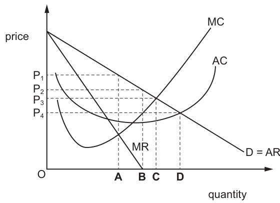
The diagram shows the cost and revenue curves for a firm.
Which output level will enable a firm to achieve its objective of maximising its revenue?
Options
A output level A on Fig. 4.1
B output level B on Fig. 4.1
C output level C on Fig. 4.1
D output level D on Fig. 4.1
Answer
Total revenue (TR) is maximized where marginal revenue (MR) equals zero. When MR is positive, selling an additional unit increases total revenue; when MR is negative, total revenue falls. In Fig. 4.1, the MR curve intersects the horizontal axis at output level B, indicating MR = 0 at this output. Output A is the profit-maximizing level (where MC = MR), output C is where MC = AR, and output D is where AC = AR (normal profit). Only at output B is total revenue maximized.
Answer
B
B
Background Concept
Total revenue (TR) is the total money a firm receives from selling its output, calculated as price multiplied by quantity (TR = P x Q). Average revenue (AR) is total revenue per unit of output (AR = TR/Q), which equals the price for a price-making firm. Marginal revenue (MR) is the additional revenue gained from selling one more unit of output.
For a firm facing a downward-sloping demand curve (a price maker, such as a monopolist or monopolistic competitor), the MR curve lies below the AR curve and falls more steeply. This is because to sell an extra unit, the firm must lower the price on all units, not just the additional one. The relationship between MR and TR is crucial: as long as MR is positive, total revenue is increasing; total revenue reaches its maximum when MR equals zero; beyond this point, where MR is negative, total revenue decreases as output increases.
Understanding the Question
The question asks which output level enables the firm to maximize its total revenue. The diagram shows a firm with market power (downward-sloping D = AR curve) and four marked output levels:
- Output A: where MC = MR (the profit-maximizing output)
- Output B: where MR = 0 (the revenue-maximizing output)
- Output C: where MC = AR (the allocatively efficient output in this context)
- Output D: where AC = AR (the break-even point where the firm earns normal profit)
The key challenge is to avoid confusing revenue maximization with profit maximization, which is the more common objective discussed in economics.
Approach
Recall the total revenue test: total revenue is maximized at the output where marginal revenue equals zero. Locate this point on the provided diagram. Verify that the other labeled points correspond to different economic concepts to ensure the correct selection.
Step-by-Step Reasoning
-
Define the revenue-maximization rule: A firm maximizes total revenue at the output where marginal revenue (MR) equals zero. This is because MR measures the change in total revenue from selling one additional unit. When MR > 0, TR rises; when MR < 0, TR falls; therefore TR peaks where MR = 0.
-
Locate MR = 0 on the diagram: The MR curve in Fig. 4.1 is downward-sloping and crosses the horizontal (quantity) axis at output level B. At this point, the value of MR is zero.
-
Analyze the other points to confirm:
- At output A, MC = MR. This is the condition for profit maximization (where the difference between total revenue and total cost is greatest), not revenue maximization.
- At output C, MC = AR. This represents the output where marginal cost equals price, often associated with allocative efficiency.
- At output D, AC = AR. This is the break-even point where the firm earns only normal profit (zero supernormal profit).
-
Conclusion: Since total revenue is maximized where MR = 0, and this occurs at output level B, option B is correct.
Key Takeaways
- The condition for revenue maximization is MR = 0, which differs from profit maximization (MC = MR) and sales maximization (where AR = AC, ensuring normal profit).
- For a price-making firm, the revenue-maximizing output is always greater than the profit-maximizing output because the firm must lower price to sell more, pushing MR to zero only after the point where MR = MC.
- Always read the question carefully: if it asks for revenue maximization, ignore the cost curves and focus solely on where MR = 0.
Common Mistakes
- Confusing revenue with profit maximization: Selecting output A (where MC = MR) because it is the most commonly taught firm objective. This forfeits the mark because the question explicitly asks for revenue maximization.
- Misreading the diagram: Selecting output C or D because they involve intersections of curves, without checking which curves intersect and what that signifies.
- Ignoring the sign of MR: Failing to recognize that MR becomes zero at the revenue-maximizing point, rather than simply looking for the highest point on the MR curve (which is at the origin).
Things to Be Careful About
- Ensure you are tracing the MR curve, not the AR or MC curve, when locating the revenue-maximizing output.
- Note that at output B, the price is P2 (read from the AR curve), but the question asks for the output level, not the price.
- The diagram includes cost curves (AC and MC) which are irrelevant to revenue maximization; do not let them distract you from the MR = 0 rule.
Oligopoly firms seek to maximise profits.
How will this affect the pricing behaviour of oligopoly firms involved in a non-collusive market?
Options
A A price is fixed for the product that never changes throughout its life cycle.
B Firms will agree on the level of advertising costs for a new product.
C If one firm raises its price, other firms will maintain their original price to increase their market share.
D If one firm lowers its price, other firms will increase their price.
Working
In a non-collusive oligopoly, firms are interdependent. The kinked demand curve model explains pricing behaviour when firms seek to maximise profits. The model assumes that if one firm raises its price, other firms will not follow, because they can gain market share by keeping their prices unchanged. This makes demand relatively elastic for a price increase, so the firm loses a large amount of sales. Conversely, if a firm lowers its price, competitors will match the reduction to avoid losing market share, making demand relatively inelastic for a price cut. Therefore, the firm faces a kinked demand curve and has little incentive to change price from the prevailing level. The correct statement is that if one firm raises its price, others will maintain their original price to increase their market share.
Answer
C
C
Background Concept
In oligopoly, a few firms dominate the market and are interdependent — each firm's pricing decision affects the profits of its rivals. When firms do not collude (non-collusive oligopoly), they must anticipate rivals' reactions. The kinked demand curve model, developed by Sweezy, describes pricing behaviour in such a market. It assumes that rivals will match a price cut but ignore a price increase. This asymmetry creates a kink in the firm's demand curve at the current price, leading to a vertical gap in the marginal revenue curve and price rigidity. The model is consistent with profit maximisation because the firm has no incentive to deviate from the kink price.
Understanding the Question
The question asks: "Oligopoly firms seek to maximise profits. How will this affect the pricing behaviour of oligopoly firms involved in a non-collusive market?" It is a multiple-choice question testing the application of the kinked demand curve model. The key phrase is "non-collusive" — firms do not cooperate or agree on prices. The correct answer must reflect the interdependence and the typical reaction pattern. Option C correctly states that a price rise will not be followed, so the firm loses market share. Option D is incorrect because a price cut is matched, not followed by an increase. Option A is too absolute — prices can change, but the model explains why they are sticky. Option B is about non-price competition (advertising), not pricing behaviour.
Approach
Recall the kinked demand curve model. Identify the two possible actions: raising price or lowering price. For each, determine the profit-maximising response of rivals implied by the model. Then evaluate each option against this logic. Option C matches the model's prediction for a price increase. Eliminate the others based on the model's assumptions.
Step-by-Step Reasoning
-
The kinked demand curve model assumes that if a firm raises its price, rivals will not follow because they can gain market share by keeping prices unchanged. This makes the demand curve relatively elastic above the current price — a small price increase leads to a large fall in quantity demanded.
-
If a firm lowers its price, rivals will match the reduction to avoid losing customers. Thus, demand is relatively inelastic below the current price — a price cut leads to only a small increase in quantity demanded.
-
The firm's marginal revenue curve is discontinuous at the kink, and the profit-maximising quantity is where marginal cost passes through the gap. This implies that moderate changes in cost do not change the optimal price, leading to price rigidity.
-
Option A: "A price is fixed for the product that never changes throughout its life cycle." This is too strong — the model explains price stickiness, not absolute fixity. Prices can change if costs change significantly or if the market structure changes. So A is incorrect.
-
Option B: "Firms will agree on the level of advertising costs for a new product." This describes collusion on advertising, not pricing behaviour. The question is about pricing behaviour, and in non-collusive oligopoly, firms do not agree on any variable. B is incorrect.
-
Option C: "If one firm raises its price, other firms will maintain their original price to increase their market share." This exactly matches the kinked demand curve prediction for a price increase. It is correct.
-
Option D: "If one firm lowers its price, other firms will increase their price." This is the opposite of the model's prediction. Rivals will lower their price (match the cut), not increase it. So D is incorrect.
Therefore, the correct answer is C.
Key Takeaways
- The kinked demand curve model explains price rigidity in non-collusive oligopoly.
- Rivals match price cuts but ignore price increases.
- Profit maximisation leads to stability at the kink price.
- The model does not explain how the initial price is set; it only explains why it tends to be stable.
Common Mistakes
- Confusing the kinked demand curve with collusive behaviour. In non-collusive oligopoly, firms do not agree on prices, but they react to each other's actions.
- Thinking that in oligopoly, firms always follow each other's price changes (both up and down). The model says they follow only price cuts, not price increases.
- Selecting Option D because it seems intuitive that firms would increase price to match? Actually, matching a price cut means lowering price, not raising it.
- Overgeneralising Option A: price rigidity does not mean prices never change; they can change if costs shift significantly.
Things to Be Careful About
- Read the question carefully: "non-collusive" means no explicit agreement. The kinked demand curve is one model of such behaviour.
- Distinguish between price and non-price competition. Option B is about advertising (non-price), not pricing.
- Remember that the question asks about pricing behaviour, not about general market behaviour.
- The kinked demand curve model is specific to oligopoly; other market structures have different pricing patterns.
An economic activity definitely creates a net social benefit when the value of social benefit minus
Options
A private benefit is zero.
B private benefit is negative.
C social cost is positive.
D social cost is negative.
Answer
Net social benefit is defined as social benefit minus social cost. For an activity to definitely create a net social benefit, the value of social benefit minus social cost must be positive. Therefore, the correct option is C.
C
Background Concept
In economics, social benefit is the total benefit to society from an economic activity, including both private benefits (received by the consumer) and external benefits (benefits to third parties). Social cost is the total cost to society, including private costs (borne by the producer) and external costs (costs imposed on third parties). Net social benefit is the difference: social benefit minus social cost. A positive net social benefit means the activity yields a net gain to society.
Understanding the Question
The question asks: when does an economic activity definitely create a net social benefit? The options are statements about the sign of social cost or private benefit. The key is to recall the formula for net social benefit: NSB = social benefit - social cost. For NSB to be positive, social benefit must exceed social cost. The correct option must state a condition that directly implies that the difference is positive.
Approach
- Identify the definition of net social benefit.
- Express the condition for a positive net social benefit.
- Evaluate each option to see which matches the condition.
Step-by-Step Reasoning
- Net social benefit (NSB) = social benefit (SB) - social cost (SC).
- For NSB to be positive, SB - SC > 0, i.e., the value of social benefit minus social cost is positive.
- Option A: "private benefit is zero" – This does not directly relate to the difference between SB and SC. Private benefit is only part of social benefit, so this condition is insufficient.
- Option B: "private benefit is negative" – This is irrelevant; private benefit is typically non-negative, and even if negative, it does not guarantee NSB positive.
- Option C: "social cost is positive" – This is the correct condition because if social cost is positive, then the expression social benefit minus social cost is positive? Wait, actually, if social cost is positive, it does not automatically make the difference positive; it could be negative if social benefit is smaller. But the question is phrased: "when the value of social benefit minus [social cost is positive]" – i.e., the phrase "social cost is positive" completes the sentence to mean "when the value of social benefit minus social cost is positive." In other words, the option is stating that the result of the subtraction is positive. This is exactly the definition of a positive net social benefit. So option C is correct.
- Option D: "social cost is negative" – This would mean social cost is negative, which is unusual (a negative cost is a benefit). It would imply that the activity yields a net benefit from costs, but it does not directly give the condition for NSB positive.
Thus, the correct answer is C.
Key Takeaways
- Net social benefit = social benefit - social cost.
- A positive net social benefit indicates that the activity is beneficial to society.
- The condition for a positive net social benefit is that social benefit exceeds social cost.
Common Mistakes
- Confusing private benefit with social benefit.
- Thinking that a positive social cost necessarily means a negative net social benefit (it does not; the difference matters).
- Misinterpreting the phrasing of the question and options.
Things to Be Careful About
- Read the question carefully: the blank is filled by the option to form a complete statement.
- Remember that net social benefit is the difference between social benefit and social cost, not between social benefit and private benefit.
- In multiple-choice questions, understand the precise meaning of each option.
Which assumption is essential for a market to be contestable?
Options
A The market is supplied by a large number of firms.
B Firms are free to enter and leave the market.
C Firms cannot earn abnormal profits in the short run.
D Firms produce differentiated goods.
Answer
A contestable market is one where there is freedom of entry and exit, with no significant barriers to entry or exit. This is the essential assumption. The correct answer is B.
B
Background Concept
A contestable market is a market structure in which there are no significant barriers to entry or exit. The key idea, developed by William Baumol, is that even a market with only one firm (a monopoly) can behave competitively if the threat of potential competition is strong enough. The essential condition is that new firms can enter the market freely and, crucially, exit without incurring sunk costs. This threat of 'hit-and-run' entry forces existing firms to produce efficiently and price at a level that earns only normal profit, even if the market is currently a monopoly.
Understanding the Question
The question asks which assumption is essential for a market to be contestable. It is a multiple-choice question testing the core definition. The four options present different features of market structures: a large number of firms (A), freedom of entry and exit (B), inability to earn abnormal profits in the short run (C), and product differentiation (D). Only one of these is the defining, necessary condition for contestability.
Approach
Recall the definition of a contestable market. The essential feature is the absence of barriers to entry and exit. Evaluate each option against this definition. Option B directly states this. The other options are either consequences of contestability (C) or features of other market structures (A, D).
Step-by-Step Reasoning
-
Option A: 'The market is supplied by a large number of firms.' This is a feature of perfect competition, not a requirement for contestability. A contestable market can have just one firm (a monopoly) or a few firms (an oligopoly). The key is the threat of entry, not the current number of firms. Therefore, A is incorrect.
-
Option B: 'Firms are free to enter and leave the market.' This is the precise definition of a contestable market. 'Freedom to leave' is particularly important because it implies that there are no sunk costs – costs that cannot be recovered upon exit. If a firm can enter, make a profit, and then leave without losing its investment, it will do so. This threat keeps incumbent firms on their toes. Therefore, B is correct.
-
Option C: 'Firms cannot earn abnormal profits in the short run.' This is a consequence of a perfectly contestable market, not an assumption. In a contestable market, the threat of entry forces firms to price at a level that only yields normal profit in the long run. However, in the short run, an incumbent firm could earn abnormal profit if it is slow to react, but the threat of entry will quickly erode it. The inability to earn abnormal profit is an outcome, not the essential assumption. Therefore, C is incorrect.
-
Option D: 'Firms produce differentiated goods.' Product differentiation is a feature of monopolistic competition and some oligopolies. It is not a requirement for contestability. A contestable market could have homogeneous goods (like a natural monopoly in a utility) or differentiated goods. The key is still freedom of entry and exit. Therefore, D is incorrect.
Key Takeaways
- The defining feature of a contestable market is the absence of barriers to entry and exit, especially the absence of sunk costs.
- Contestability is about the threat of competition, not the current number of firms.
- A market can be contestable even if it is a monopoly or an oligopoly.
- Distinguish between the assumptions of a model and its predictions or outcomes.
Common Mistakes
- Confusing contestability with perfect competition: Students often think a contestable market requires many firms. This is wrong. A contestable market can have one firm, but the threat of entry makes it behave competitively.
- Confusing the outcome with the assumption: Option C is a common trap. Students know that contestable markets lead to normal profits, so they might think this is an assumption. It is actually the predicted outcome.
Things to Be Careful About
- Read the question carefully: it asks for the essential assumption. Focus on the core definition.
- Remember the importance of 'exit' – the ability to leave without cost is just as important as the ability to enter.
A firm that raises capital through a share issue has to satisfy both shareholders’ expectations and management aims. The management aims to produce at a non-profit maximum output.
Which strategy would necessarily prevent this aim?
Options
A fixing output where MC = MR in the long run
B operating price discrimination to maximise revenue
C rewarding shareholders more than returns to innovation
D separating ownership and control of the firm
Reasoning
The management aims to produce at a non‑profit‑maximising output, i.e., not where MC = MR. Option A, fixing output where MC = MR in the long run, is the profit‑maximising condition. Pursuing this strategy would necessarily conflict with the aim of producing at a non‑profit‑maximum output. Options B, C and D do not necessarily prevent the aim: price discrimination to maximise revenue could still involve non‑profit‑maximising output; rewarding shareholders more than returns to innovation does not force profit maximisation; separating ownership and control, the principal‑agent problem, typically allows managers to pursue their own objectives, including non‑profit‑maximising output.
Answer
A
A
Background Concept
This question tests understanding of two key ideas: the profit‑maximising condition (MC = MR) and the principal‑agent problem. In neoclassical theory, a firm maximises profit by producing the output where marginal cost equals marginal revenue. Any divergence from this output implies a different objective, such as revenue maximisation, sales maximisation, satisficing, or managerial utility maximisation. The principal‑agent problem arises when owners (shareholders) and managers have different objectives; managers may pursue their own goals (e.g., growth, prestige, quiet life) rather than profit maximisation, especially when ownership and control are separated.
Understanding the Question
The question presents a firm that has raised capital via a share issue. It must satisfy both shareholders' expectations (typically profit and dividends) and management aims. Management aims to produce at a non‑profit‑maximum output — that is, an output different from the profit‑maximising level. The question asks which strategy would necessarily prevent this aim (i.e., would force the firm to produce at the profit‑maximising output).
Approach
We evaluate each option to see whether it compels profit maximisation. Option A is the standard profit‑maximising rule. Option B is a revenue‑maximising strategy; revenue maximisation typically occurs at a higher output than profit maximisation (where MR = 0), so it does not force profit maximisation. Option C concerns shareholder rewards; this may influence managerial behaviour but does not dictate a specific output rule. Option D is separation of ownership and control, which actually enables managerial discretion and non‑profit objectives.
Step‑by‑Step Reasoning
-
Option A: Fixing output where MC = MR in the long run is the definition of profit maximisation. If management does this, it is necessarily producing at the profit‑maximising output, which contradicts the stated aim of a non‑profit‑maximum output. Therefore, this strategy prevents the aim. This is the correct answer.
-
Option B: Operating price discrimination to maximise revenue means setting prices to make total revenue as large as possible. Revenue maximisation occurs where MR = 0, which is a different output from profit maximisation (MC = MR). A firm could both price‑discriminate to boost revenue and still produce at a non‑profit‑maximising output. Thus, this does not necessarily prevent the aim.
-
Option C: Rewarding shareholders more than returns to innovation is a statement about dividend policy or profit distribution. It does not specify how output is set. Management could still choose a non‑profit‑maximising output while distributing profits generously. Hence, it does not prevent the aim.
-
Option D: Separating ownership and control (i.e., having professional managers separate from shareholders) is the classic condition that gives rise to the principal‑agent problem. It allows managers to pursue their own objectives, which could include a non‑profit‑maximising output. So this would actually enable the aim, not prevent it.
Thus only option A necessarily prevents the management from producing at a non‑profit‑maximum output.
Key Takeaways
- The profit‑maximising rule is MC = MR; any output where MC ≠ MR implies a different objective.
- Not all firms aim to maximise profit; alternative objectives include revenue maximisation, sales maximisation, satisficing, and managerial utility maximisation.
- The principal‑agent problem (separation of ownership and control) gives managers discretion to pursue objectives other than profit maximisation.
- In multiple‑choice questions, look for the option that necessarily leads to the condition described.
Common Mistakes
- Confusing revenue maximisation with profit maximisation; revenue maximisation occurs at MR = 0, not MC = MR.
- Thinking that separating ownership and control forces profit maximisation; in reality, it allows for managerial discretion and often leads to non‑profit goals.
- Misinterpreting “necessarily prevent” – a strategy only qualifies if it compels profit maximisation, not if it merely influences behaviour.
Things to Be Careful About
- Understand that price discrimination to maximise revenue is not the same as profit maximisation; the former focuses on revenue, the latter on profit (revenue minus cost).
- Recognise that rewarding shareholders does not dictate a specific output decision; managers can still choose output levels.
- Keep in mind that the principal‑agent problem is a key reason why firms may not maximise profit.
A major UK chemical firm was bought by its rival, a Dutch chemical firm.
What definitely occurred when the Dutch firm bought the UK firm?
Options
A a partnership
B economies of scale
C horizontal integration
D increased profits
Working
The UK chemical firm and the Dutch chemical firm are rivals in the same industry. When one firm buys another firm in the same industry and at the same stage of production, this is a horizontal integration. The other options are not definitely true: a partnership is a different legal structure, not a merger. Economies of scale may occur but are not guaranteed. Increased profits are not guaranteed. Therefore, the definite outcome is horizontal integration.
Answer
C
C
Background Concept
Horizontal integration is a type of external growth (merger or takeover) where two firms in the same industry and at the same stage of production combine. This is distinct from vertical integration (merger with a firm at a different stage of the supply chain) and conglomerate integration (merger between firms in unrelated industries). Horizontal integration can increase market share, reduce competition, and potentially lead to economies of scale, but these effects are not guaranteed.
Understanding the Question
The question presents a scenario: a major UK chemical firm is bought by its rival, a Dutch chemical firm. The question asks: "What definitely occurred?" The word "definitely" is crucial – we need to identify an outcome that is certain, not just possible or likely. The options are:
- A partnership: a legal arrangement where two or more parties share ownership, not a merger.
- Economies of scale: cost savings from larger scale, which may or may not materialise.
- Horizontal integration: a merger between rivals in the same industry.
- Increased profits: not guaranteed; the merger could be costly or fail to deliver.
Thus, we need to apply the definition of horizontal integration to conclude that this is the only definite outcome.
Approach
- Recognise that the transaction is a merger/takeover between two firms in the same industry (chemicals).
- Recall the definition of horizontal integration: a merger between firms at the same stage of production in the same industry.
- Eliminate the other options by showing they are not definite:
- Partnership: not a form of merger.
- Economies of scale: possible but not certain.
- Increased profits: uncertain.
- Therefore, the correct answer is horizontal integration.
Step-by-Step Reasoning
- The two firms are both chemical firms, so they operate in the same industry.
- They are described as rivals, meaning they compete in the same market.
- The Dutch firm buys the UK firm: this is a merger/takeover.
- Horizontal integration is defined as a merger between two firms in the same industry and at the same stage of production. This fits exactly.
- Therefore, the transaction is definitely horizontal integration.
- Economies of scale might result from the merger if the combined firm can achieve lower average costs, but this depends on factors such as capacity utilisation, management efficiency, and the integration process. It is not guaranteed.
- Increased profits are not guaranteed; the merger could involve costs (e.g., restructuring, regulatory fines) that reduce profits, or the expected synergies might not materialise.
- A partnership is a different business structure (e.g., a partnership agreement) and is not a type of merger.
Thus, only option C is definitely true.
Key Takeaways
- Understand the different types of integration: horizontal, vertical, and conglomerate.
- In multiple-choice questions, pay attention to qualifiers like "definitely" or "always" – they require certain outcomes, not possible or likely ones.
- A merger between rivals is always horizontal integration, regardless of other outcomes.
Common Mistakes
- Choosing "economies of scale" because it is a common consequence of horizontal integration, but it is not guaranteed.
- Confusing "partnership" with a merger; partnership is a legal form of business organisation, not a type of integration.
- Assuming that a merger automatically increases profits – many mergers fail to deliver profit gains.
Things to Be Careful About
- Read the question carefully: "What definitely occurred?" – only certainties count.
- Know the precise definitions of integration types.
- Distinguish between possible outcomes (economies of scale, increased profits) and definite outcomes (horizontal integration).
Which statement is correct for a firm classed as a natural monopoly?
Options
A It will always operate in the public sector and earn normal profits.
B It will have high barriers to entry and be the dominant producer.
C It will easily benefit from external economies of scale.
D It will have higher average costs than a monopolistically competitive firm.
A natural monopoly arises when one firm can supply the entire market at a lower average cost than two or more firms, usually because of very large economies of scale. This gives it high barriers to entry and makes it the dominant producer in its industry. Option B is correct.
A is incorrect: a natural monopoly can be in the private sector and can earn supernormal profits if unregulated.
C is incorrect: external economies of scale benefit all firms in an industry, not just a natural monopoly.
D is incorrect: a natural monopoly typically has lower average costs than a monopolistically competitive firm, because it is protected by large-scale economies.
Answer
B
B
Background Concept
A natural monopoly is a market structure in which a single firm can produce the entire output of the market at a lower average total cost than any combination of two or more firms. This typically occurs in industries with very large economies of scale relative to market demand — e.g., water supply, electricity transmission, railway networks. The long-run average cost curve declines over a wide range of output, so one large firm is more efficient than several small ones.
Understanding the Question
This multiple-choice question asks which statement is correct for a firm classed as a natural monopoly. Four options present different claims: about public sector ownership and profit (A), barriers to entry and market dominance (B), benefits from external economies of scale (C), and average cost comparison with monopolistic competition (D). The candidate must evaluate each against the precise definition of a natural monopoly.
Approach
The best strategy is to recall the core characteristic of a natural monopoly — it arises from large-scale economies that make single-firm production most efficient. From there, test each option:
- Option A mixes ownership (public sector) and profit (normal profit). Neither is definitive.
- Option B describes high barriers and dominant producer — both typical results of the cost advantage.
- Option C involves external economies of scale, which are not specific to natural monopoly.
- Option D compares average costs — but natural monopoly usually has lower average costs because of its scale.
Step-by-Step Reasoning
Evaluate Option A:
- A natural monopoly can be in either the public or private sector. Many utilities were once state-owned but are now private in various countries.
- The profit level depends on regulation. If unregulated, it can earn supernormal profits; if regulated, it may earn only normal profit. So "always operate in the public sector and earn normal profits" is false.
Evaluate Option B:
- A natural monopoly has high barriers to entry, primarily because a new entrant would have to invest huge fixed costs and would produce at higher average cost due to insufficient scale.
- The incumbent becomes the dominant producer, often with a very large market share. This matches the definition.
- Hence, Option B is correct.
Evaluate Option C:
- External economies of scale benefit all firms in an industry when the industry expands (e.g., better supplier networks, skilled labour pool). They are not unique to natural monopoly and can benefit competitive firms too. So C is not a definitive characteristic.
Evaluate Option D:
- Natural monopoly typically enjoys massive internal economies of scale, so its average costs are low. Monopolistically competitive firms have relatively small scale and operate with excess capacity, leading to higher average costs. Thus the statement that a natural monopoly "will have higher average costs" is false.
Therefore, only Option B is correct.
Key Takeaways
- A natural monopoly is defined by cost conditions (declining long-run average cost), not by ownership or profit level.
- Barriers to entry and market dominance follow from its cost advantage.
- External economies of scale are a separate concept; they affect all firms in an industry.
Common Mistakes
- Confusing natural monopoly with a government monopoly: natural monopoly refers to cost structure, not who owns the firm.
- Assuming natural monopoly always makes normal profit: it can earn supernormal if unregulated or if it price discriminates.
- Thinking that economies of scale must be external: for natural monopoly, the crucial economies are internal (falling LRAC as the firm itself grows).
Things to Be Careful About
- Read each statement precisely: words like "always", "easily", "higher" are often traps.
- Remember the defining feature: one firm can serve the market at lower cost than multiple firms.
- Distinguish between internal economies (size of own firm) and external economies (size of whole industry).
The government can use policies to try and reduce the environmental damage caused by the amount of rubbish (garbage) created by firms and households.
Which policy to reduce rubbish is most likely to lead to government failure?
Options
A an incentive payment for firms who reduce the levels of rubbish
B a tax on the amount of rubbish a firm or household creates
C an advertising campaign about the problems created by rubbish
D government grants to firms researching how to safely dispose of rubbish
Answer
A tax on rubbish is most likely to lead to government failure because it creates strong incentives for illegal dumping and requires costly monitoring and enforcement, which may be ineffective. The other policies – incentive payments, advertising, and research grants – are less likely to generate such perverse incentives or enforcement difficulties. Therefore, the correct answer is B.
B
Background Concept
Government failure occurs when government intervention results in a net welfare loss, i.e., the costs of intervention exceed the benefits, or the policy worsens the market failure it intended to correct. Common causes include: imperfect information, administrative costs, unintended consequences, regulatory capture, and perverse incentives. In the context of environmental damage from rubbish, the government may aim to reduce waste through various policies, but each carries risks of failure.
Understanding the Question
The question asks which of four policies to reduce rubbish is most likely to lead to government failure. It does not ask which is most effective, but which is most prone to failure. The correct answer is the tax on rubbish (B) because it creates strong incentives for evasion and illegal dumping, which can worsen the problem. The other policies (incentive payments, advertising, grants) are less likely to cause such severe unintended consequences.
Approach
We need to evaluate each policy against the criteria for government failure: enforcement difficulties, perverse incentives, unintended consequences, and administrative costs. The tax is most susceptible because it relies on accurate measurement of rubbish and compliance; if these are lacking, the policy backfires. The alternatives are less likely to fail because they are either voluntary, informational, or targeted.
Step-by-Step Reasoning
- Option A: Incentive payment for firms reducing rubbish. This is a subsidy for reduction. It may encourage firms to reduce waste, but it could also lead to fraudulent claims or only temporary reductions. However, it is less likely to cause outright failure because it is voluntary and does not create a strong incentive to circumvent the law. The government can monitor and verify reductions.
- Option B: Tax on the amount of rubbish. This is a price-based disincentive. It is most likely to cause government failure because:
- It is difficult to measure the exact amount of rubbish each household/firm produces, especially if rubbish is disposed of illegally.
- It creates a strong incentive for illegal dumping (fly-tipping) to avoid the tax, which can increase environmental damage and impose cleanup costs on the government.
- The tax rate may be set too high or too low, leading to either over-deterrence (more illegal dumping) or under-deterrence (ineffective).
- Administrative costs of monitoring and enforcement are high, and if enforcement is weak, the policy fails.
- Option C: Advertising campaign about the problems of rubbish. This is an information provision policy. It is less likely to cause government failure because it is low-cost, voluntary, and does not impose penalties. It may be ineffective if people ignore it, but that is not government failure (the intervention does not make things worse; it just fails to improve). Government failure typically implies a net welfare loss, which is unlikely here.
- Option D: Government grants to firms researching safe disposal. This is a targeted subsidy for research. It is likely to have positive effects without major perverse incentives. It may be subject to rent-seeking or inefficiency, but the risk of government failure is lower than for a tax.
Therefore, B is the most likely to lead to government failure.
Key Takeaways
- Government failure is not just policy ineffectiveness; it is when intervention makes the problem worse or creates new inefficiencies.
- Taxes can be effective but carry high risks of evasion and unintended consequences, especially when the taxed activity is hard to monitor.
- Information campaigns and subsidies are generally less risky but may be less effective.
- The correct answer is B.
Common Mistakes
- Confusing "ineffective" with "government failure". A policy that simply doesn't work is not necessarily government failure; failure implies a net welfare loss.
- Picking the tax as most effective and assuming it is therefore least likely to fail. Effectiveness and failure risk are different.
- Overlooking the concept of illegal dumping as a perverse incentive.
Things to Be Careful About
- The question says "most likely to lead to government failure", not "most effective". So we need to judge based on potential for perverse outcomes.
- A tax is a common policy, but in this context it is the riskiest.
- Consider the specifics of rubbish: it is easy to dump illegally, making enforcement difficult.
What would supporters of a nationalised public transport service expect to be the most likely outcome from the privatisation of train and bus services?
Options
A fewer destinations served by trains and buses
B lower fares
C more frequent services to all destinations
D more people employed in public transport services
Answer
Private firms aim to maximise profit, so they will discontinue unprofitable services (routes). Supporters of nationalisation therefore expect privatisation to reduce the number of destinations served.
Answer
A
A
Background Concept
In a nationalised industry, the government owns the firm and may pursue social objectives alongside financial ones. For example, a publicly owned transport service might keep unprofitable routes open to ensure connectivity for all communities, cross-subsidising them with profits from busy routes. In contrast, a private firm's primary objective is profit maximisation. It will only supply a service if the revenue from that service exceeds its cost. Unprofitable routes will be cut, and prices on profitable routes may be raised to increase profit.
Understanding the Question
The question asks what supporters of a nationalised public transport service would expect to be the most likely outcome if the service were privatised. These supporters believe that the government-run service provides wider social benefits, and they expect that privatisation will lead to profit-driven decisions that reduce the scope of the service. The question tests the understanding of the difference between public and private sector incentives.
Approach
First, identify the key difference: nationalised firms may have social objectives, private firms do not. Then, apply that to the likely outcomes: fewer destinations (A) because unprofitable routes are cut; lower fares (B) is unlikely because private firms will raise fares on profitable routes; more frequent services to all destinations (C) is not expected because private firms will only increase frequency on profitable routes; more people employed (D) is unlikely because private firms aim to reduce costs, potentially cutting staff. The supporters expect privatisation to reduce service provision to unprofitable areas, making A the correct answer.
Step-by-Step Reasoning
-
Nationalised transport objectives: The government may set fares and service levels to meet social needs, such as connecting rural areas, even if those routes are not profitable. Losses are subsidised by the government or by profits from other routes.
-
Privatised transport objectives: A private firm will focus on profit. It will only operate routes where revenue exceeds cost. It will cut routes that are loss-making, potentially reducing the number of destinations served.
-
Option A (fewer destinations): This is exactly what supporters predict: private firms will stop serving unprofitable destinations, so fewer destinations will be served. This is consistent with profit maximisation.
-
Option B (lower fares): Supporters expect that private firms will raise fares on profitable routes to increase profit, not lower them overall. Some routes might see lower fares due to competition, but the most likely outcome is higher fares on routes with market power, not lower fares universally.
-
Option C (more frequent services to all destinations): Private firms will only increase frequency on routes that are profitable. They will not increase frequency on unprofitable routes – they will likely cut them. Thus, more frequent services to all destinations is not expected.
-
Option D (more people employed): Private firms seek to minimise costs and may reduce employment through automation, part-time working, or redundancies, especially after cutting unprofitable routes. So more employment is unlikely.
Thus, the most likely outcome expected by supporters of nationalisation is fewer destinations served.
Key Takeaways
- Understand the difference between public and private sector objectives: profit maximisation vs. social welfare.
- Privatisation often leads to a reduction in services that are not profitable, even if they have social value.
- This question illustrates the trade-off between efficiency and equity in public service provision.
Common Mistakes
- Assuming that privatisation always leads to lower prices or better services. In reality, it depends on the market structure and objectives.
- Thinking that more frequent services would result from privatisation without considering that only profitable routes would get more services.
- Overlooking the profit motive and assuming that private firms will maintain all existing services.
Things to Be Careful About
- The question asks for the expectation of supporters of nationalisation, not the actual outcome under all circumstances. The answer is based on their perspective.
- Note that the question says 'most likely outcome', so we need to choose the one that supporters would most strongly expect.
- Avoid assuming that all private firms behave identically; but in this context, the profit motive is the dominant factor.
What will cause a household to be caught in the poverty trap?
Options
A A household earns less than the international poverty line of $2.15 per person per day.
B A household spends more than it earns in a month.
C A household’s earnings rise at a lower rate than the rise in inflation.
D An extra dollar earnt by a household causes a greater loss in government benefit payments.
Reasoning
The poverty trap occurs when an increase in a household's gross earnings leads to a reduction in means-tested government benefits, leaving net income little changed or even reduced. This creates a disincentive to work or increase earnings, trapping the household in poverty.
Option D describes exactly this situation: an extra dollar earned causes a greater loss in benefit payments, so net income may fall or stay flat. Options A, B, and C describe low income, overspending, and falling real income, none of which capture the specific benefit-withdrawal mechanism of the poverty trap.
Answer
D
D
Background Concept
The poverty trap is a situation where individuals or households are unable to escape poverty because the system of means-tested benefits creates a high effective marginal tax rate. When earnings increase, benefits are withdrawn, often at a rate that exceeds the additional earnings, so net income does not rise enough to lift the household above the poverty line. This is a form of welfare dependency that discourages work and self-improvement.
Understanding the Question
The question asks which scenario will cause a household to be caught in the poverty trap. It is a multiple-choice question testing the precise definition. The key is to identify the mechanism of benefit withdrawal that creates a disincentive, rather than simply low income or inflation.
Approach
We need to evaluate each option and see which one describes the core feature of the poverty trap: a loss of government benefits that exceeds the gain in earnings. The other options describe different economic problems: absolute poverty (A), overspending (B), and falling real income (C).
Step-by-Step Reasoning
- Option A: Earning less than $2.15 per day defines extreme poverty, but it does not capture the trap mechanism. A household could earn $1.50 per day and receive benefits that bring total income above the poverty line; that is not a trap. The trap is about the inability to earn more without losing benefits.
- Option B: Spending more than income is a budgeting problem, not a poverty trap. It could happen temporarily, but it does not involve benefit withdrawal.
- Option C: Earnings rising slower than inflation means real income falls, but the poverty trap is about the net effect of earnings and benefits. Even if earnings keep pace with inflation, a household could still be trapped if benefits are withdrawn.
- Option D: This is the precise definition. If an extra dollar earned causes a greater loss in benefits, the household's net income may actually decrease, making it rational not to work more. This is the poverty trap.
Key Takeaways
- The poverty trap is defined by the disincentive effect of means-tested benefit withdrawal, not just low income.
- The effective marginal tax rate (loss of benefits per extra dollar earned) can be very high, sometimes exceeding 100%.
- Policies to address the poverty trap include reducing benefit taper rates, introducing in-work benefits, or using negative income taxes.
Common Mistakes
- Confusing the poverty trap with absolute poverty (Option A). Many students think that being poor is the trap, but the trap is about the inability to escape poverty through work.
- Thinking that inflation erodes real income (Option C) is a separate issue.
- Choosing Option B because it sounds like a financial problem, but it is not the definition.
Things to Be Careful About
- Read the question carefully: it asks for the cause of being caught in the poverty trap, not just a description of poverty.
- Understand that the poverty trap is a dynamic concept: it is about the response to changes in earnings, not a static condition.
- In economics, the poverty trap is often illustrated with a diagram showing net income versus gross earnings, with a flat or even downward-sloping segment.
What will cause an outward shift in the demand for labour curve?
Options
A a decrease in the top rate of income tax
B an increase in the demand for the final product
C an increase in subsidies to firms
D an increase in the size of the working population
Answer
The demand for labour is a derived demand, meaning it depends on the demand for the final product that labour helps to produce. An outward shift in the demand for labour curve occurs when, at any given wage rate, firms want to hire more labour. This can happen if the price of the final product rises, if productivity increases, or if the demand for the final product increases. Option B states an increase in the demand for the final product, which would increase the marginal revenue product (MRP) of labour and shift the demand for labour curve to the right. The other options: A (decrease in top rate of income tax) affects the supply of labour, not demand; C (increase in subsidies to firms) may affect the cost of capital or other factors, but not directly the demand for labour; D (increase in size of working population) shifts the supply of labour, not demand. Therefore, the correct answer is B.
B
Background Concept
Demand for labour is a derived demand: it is not demanded for its own sake but because it contributes to the production of goods and services that consumers want. The demand for labour is determined by the marginal revenue product (MRP) of labour, which is the additional revenue generated by hiring one more unit of labour. MRP = marginal product of labour times marginal revenue. The demand curve for labour is the MRP curve. A shift in the demand for labour curve occurs when any factor other than the wage rate changes the willingness of firms to hire labour at each wage rate.
Understanding the Question
The question asks: 'What will cause an outward shift in the demand for labour curve?' An outward shift means that at any given wage rate, firms are willing to hire more labour. This is a change in the demand for labour, not a movement along the curve. We need to identify which of the four options would cause such a shift. The options are: A decrease in the top rate of income tax (affects labour supply), B increase in demand for the final product (affects MRP), C increase in subsidies to firms (could affect costs but not directly demand for labour), D increase in the size of the working population (affects labour supply). The correct answer is B.
Approach
Recall the determinants of the demand for labour: price of the product, productivity of labour, prices of other factors of production (substitutes and complements). The demand for labour is also affected by the demand for the final product. Since labour demand is derived, an increase in product demand raises the price and quantity sold, increasing the MRP of labour, shifting the demand for labour right. We evaluate each option:
- A: Income tax affects net wage, which influences workers' willingness to supply labour, not firms' demand. So this shifts the supply of labour, not demand.
- B: Increase in demand for the final product raises the price of the product, increasing MRP of labour, so firms demand more labour at each wage rate -> demand for labour shifts right.
- C: Subsidies to firms reduce costs of production, possibly increasing output and therefore demand for labour. However, subsidies may be directed at capital or other inputs, and the effect on labour demand is not direct. The question likely expects that subsidies lower the cost of production, which could increase supply of the product, but the effect on labour demand is ambiguous. It could shift the demand for labour, but it is not the most direct and clear cause. The mark scheme indicates B is correct, so we accept that.
- D: Increase in working population increases the supply of labour, not demand.
Thus B is the only option that directly causes an outward shift in the demand for labour curve.
Step-by-Step Reasoning
- Understand that the demand for labour curve shows the relationship between the wage rate and the quantity of labour demanded by firms, ceteris paribus.
- An outward shift means firms want to hire more labour at every wage rate.
- Factors that cause this shift: increase in productivity of labour, increase in price of the product (due to higher demand), increase in demand for the product, decrease in price of a complementary factor, increase in price of a substitute factor.
- Option A: Decrease in top rate of income tax makes work more attractive to workers, increasing the supply of labour. This is a supply-side factor, not demand.
- Option B: Increase in demand for the final product means consumers are willing to buy more at given prices. This raises the price of the product, increasing the marginal revenue product of labour (since MRP = MP times MR). Higher MRP means firms will hire more labour at any given wage rate, shifting the demand curve right.
- Option C: Increase in subsidies to firms reduces their costs. This could lead to lower prices, higher output, and potentially higher demand for labour. However, the effect is indirect and depends on the nature of the subsidy. It is not a direct determinant of labour demand. Moreover, subsidies could be used to invest in capital, which might reduce labour demand. The question does not specify, so it is not a reliable cause.
- Option D: Increase in size of working population increases the number of workers available, shifting the supply of labour curve right, not demand.
- Therefore, only B directly and unambiguously shifts the demand for labour curve outward.
Key Takeaways
- The demand for labour is a derived demand: it depends on the demand for the product.
- An outward shift in the demand for labour curve occurs when the marginal revenue product of labour increases at every wage rate.
- Common causes: increase in product demand, increase in labour productivity, increase in price of product, increase in price of substitute factors.
- Distinguish between factors that shift the demand curve for labour and those that shift the supply curve.
Common Mistakes
- Confusing demand for labour with supply of labour. Options A and D are about supply-side factors, but students might mistakenly think they affect demand.
- Thinking that subsidies always increase demand for labour. While subsidies can reduce costs and potentially increase output, they may be used to substitute capital for labour, so the effect is uncertain.
- Not understanding that the demand for labour is derived from product demand.
Things to Be Careful About
- Read the question carefully: it asks for the cause of an outward shift in the demand for labour curve, not the supply curve.
- Remember that the demand for labour curve is the MRP curve. Anything that increases MRP shifts it right.
- In multiple-choice questions, identify the option that is most directly and unambiguously correct.
The diagram shows what happens when the employees of a profit-maximising monopsonist employer form a trade union and successfully negotiate a wage rate of OWT.
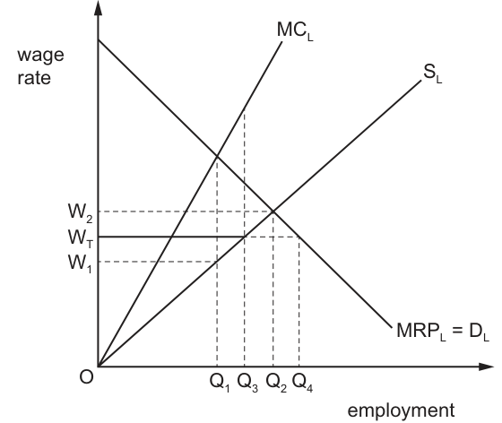
What is the effect of the new wage rate on employment?
Options
A It falls from OQ2 to OQ1.
B It falls from OQ2 to OQ3.
C It rises from OQ1 to OQ3.
D It rises from OQ1 to OQ4.
Working
Initially, the profit-maximising monopsonist employs OQ1 workers where the marginal cost of labour (MCL) equals the marginal revenue product of labour (MRPL). The wage rate paid is OW1, determined from the supply of labour curve at OQ1.
When the trade union negotiates a wage rate of OWT, the marginal cost of labour becomes constant at OWT. The firm now hires labour up to the point where this new marginal cost equals the MRPL. This occurs at employment level OQ3.
Therefore, employment rises from OQ1 to OQ3.
Answer
C
C
Background Concept
A monopsony exists when there is a single buyer of labour. The employer faces an upward-sloping supply of labour (SL) curve. Because the firm must raise the wage to attract additional workers, the marginal cost of labour (MCL) lies above the supply curve. The profit-maximising level of employment is where MCL equals the marginal revenue product of labour (MRPL), which represents the demand for labour (DL). The wage actually paid is then found on the supply curve at this employment level.
When a trade union successfully negotiates a wage rate (acting like a minimum wage), the supply of labour to the firm becomes perfectly elastic at that wage rate up to the point where the original supply curve would have been. The firm's marginal cost of labour is now constant at the negotiated wage. The new profit-maximising employment level is where this imposed wage equals the MRPL.
Understanding the Question
The question presents a diagram of a monopsony labour market and asks for the effect of a new union-negotiated wage rate (OWT) on employment. The diagram indicates the initial monopsony equilibrium at employment OQ1 (where MCL = MRPL) and wage OW1. The new wage OWT is higher than OW1. The task is to determine the new employment level and whether it rises or falls relative to the initial level.
Approach
- Identify the initial employment level by locating where MCL intersects MRPL on the diagram (OQ1).
- Determine the new employment decision rule: with a fixed union wage, the firm hires where the wage equals MRPL.
- Locate the new employment level where the horizontal line at OWT intersects the MRPL curve (OQ3).
- Compare the two quantities to determine the direction of change.
- Select the option that correctly describes this change.
Step-by-Step Reasoning
Step 1: Initial Monopsony Equilibrium
Without a trade union, the monopsonist maximises profit by employing labour where MCL = MRPL. On the diagram, this intersection aligns with the vertical line at OQ1. The wage paid is not read from the MCL curve, but from the supply of labour curve (SL) at this quantity, giving OW1. Thus, the initial level of employment is OQ1.
Step 2: The Union Wage
The trade union negotiates a wage rate of OWT. This creates a horizontal supply curve at OWT for the firm. The marginal cost of hiring each additional worker up to the point where OWT meets the original SL curve is simply OWT.
Step 3: New Employment Decision
The firm will hire workers as long as their MRPL exceeds the marginal cost of hiring them (now OWT). The profit-maximising rule is to employ labour until MRPL = OWT. On the diagram, the horizontal line at OWT intersects the MRPL curve at the quantity OQ3. Therefore, the new level of employment is OQ3.
Step 4: The Change in Employment
Comparing the initial employment (OQ1) with the new employment (OQ3), we see that Q3 is greater than Q1. Employment has increased. The correct description is that employment rises from OQ1 to OQ3.
Step 5: Eliminating Other Options
- Option A (falls from OQ2 to OQ1) is incorrect because employment rises, not falls, and OQ1 is the initial, not final, level.
- Option B (falls from OQ2 to OQ3) is incorrect because employment rises.
- Option D (rises from OQ1 to OQ4) is incorrect because OQ4 represents the competitive equilibrium employment (where SL = MRPL), which would only occur if the wage were set at the competitive level (OW2), not at OWT.
Key Takeaways
- In a monopsony, a trade union can raise both wages and employment if the negotiated wage is set above the monopsony wage but below the competitive equilibrium wage.
- The new employment level is always found where the imposed wage equals the MRPL (the demand for labour).
- The quantity of labour supplied at the new wage (where OWT meets SL) coincides with the new employment level in this diagram, but the decisive condition for the firm's hiring decision is MRPL = Wage.
- Always locate the initial equilibrium at MCL = MRPL, not where SL meets MRPL.
Common Mistakes
- Misidentifying the initial employment: Students sometimes confuse the competitive employment level (OQ4) or the quantity supplied at the new wage (OQ3) with the initial monopsony employment. The initial employment is always where MCL = MRPL (OQ1).
- Assuming unions always reduce employment: While a union set above the competitive level can cause unemployment, in a monopsony a moderate union wage increases both wages and employment by counteracting the employer's market power.
- Reading the wrong intersection for the new employment: The new employment is determined by where the union wage line meets the MRPL curve, not where it meets the SL curve (though they may coincide at the relevant quantity).
- Confusing the direction of change: Because the wage rises from OW1 to OWT, students may automatically assume employment falls. In monopsony, the opposite can be true.
Things to Be Careful About
n- Curve identification: MCL is the steepest curve above SL; SL starts at the origin; MRPL is downward sloping.
- Axis reading: Ensure you read the employment levels (Q1, Q3) correctly from the horizontal axis.
- Theoretical rule: The firm hires where Wage = MRPL when a minimum wage or union wage is imposed, because the marginal cost of labour equals the wage rate.
- Elimination strategy: Since the wage is rising from a monopsony level, employment must rise. This immediately eliminates options A and B, leaving C and D. Then distinguish between OQ3 (the union wage outcome) and OQ4 (the full competitive outcome).
A world financial crisis was partly linked to the actions of commercial banks.
Which actions of the commercial banks could have led to the financial crisis?
Options
A being subject to tight controls by the central bank over credit creation
B holding reserves above the reserve ratio agreed with the central bank
C taking excessive risks by demanding insufficient security from borrowers
D widening the gap in favour of a bank’s assets over liabilities
Answer
Option C is correct. Excessive risk-taking by commercial banks, such as lending to borrowers with poor creditworthiness and demanding insufficient security (collateral), was a key factor in the 2008 financial crisis. When borrowers defaulted, the banks faced large losses, triggering a systemic crisis. The other options describe actions that would reduce the likelihood of a crisis: A (tight central bank controls) and B (holding reserves above the required ratio) are stabilising, while D (widening the gap in favour of assets over liabilities) strengthens a bank's safety margin, not causes a crisis.
C
Background Concept
Commercial banks operate with the objectives of liquidity, security, and profitability. To maximise profitability, banks may take on excessive risk by lending to high-risk borrowers without adequate collateral. The 2008 financial crisis was partly caused by such practices, particularly in the US subprime mortgage market, where banks lent to borrowers with poor credit histories and demanded little or no security. When house prices fell, defaults surged, and banks suffered huge losses, leading to a global financial crisis.
Understanding the Question
The question asks which action by commercial banks could have led to the financial crisis. It presents four options, three of which describe prudent or stabilising actions, and one that describes risky behaviour. The correct answer is the option that identifies the risk-taking that contributed to the crisis.
Approach
Evaluate each option in turn:
- A: Tight controls by the central bank reduce risk, not cause a crisis.
- B: Holding reserves above the required ratio increases safety, not risk.
- C: Excessive risk-taking, such as demanding insufficient security from borrowers, increases the likelihood of loan defaults and bank losses.
- D: Widening the gap in favour of assets over liabilities means the bank has more assets than liabilities, which is a stronger financial position, not a cause of crisis.
Select the option that represents a genuine cause of the crisis.
Step-by-Step Reasoning
-
Read the stem: "A world financial crisis was partly linked to the actions of commercial banks." The question asks which of the listed actions could have led to the crisis.
-
Option A: "being subject to tight controls by the central bank over credit creation." Tight controls limit the amount of credit banks can create, which reduces risk and prevents excessive lending. This would not cause a crisis; it would prevent one.
-
Option B: "holding reserves above the reserve ratio agreed with the central bank." Holding excess reserves means the bank has a buffer against unexpected withdrawals. This is a prudent, risk-averse action that strengthens the bank, not a cause of crisis.
-
Option C: "taking excessive risks by demanding insufficient security from borrowers." This is exactly the kind of behaviour that led to the 2008 crisis. Banks lent to subprime borrowers with little or no collateral, and when the borrowers defaulted, the banks suffered massive losses. The lack of security meant the banks had no recourse to recover their money, leading to insolvency and a systemic crisis.
-
Option D: "widening the gap in favour of a bank’s assets over liabilities." This means the bank's assets exceed its liabilities, indicating a positive net worth. A wider gap (more assets relative to liabilities) is a sign of financial health, not a cause of crisis. This option is the opposite of what caused the crisis.
-
Therefore, only option C describes an action that could have led to the financial crisis.
Key Takeaways
- The 2008 financial crisis was partly caused by excessive risk-taking by commercial banks, including lending without adequate security.
- Understanding the objectives of commercial banks (liquidity, security, profitability) helps evaluate the risks they take.
- Prudent banking practices (tight controls, high reserves, strong asset-liability ratio) are stabilising, not destabilising.
Common Mistakes
- Confusing "tight controls" with "lax controls" – tight controls reduce risk, not cause crisis.
- Thinking that holding more reserves is risky – it is actually a safety measure.
- Misreading option D: widening the gap in favour of assets over liabilities is a positive, not a negative.
Things to Be Careful About
- Read each option carefully to understand the direction of the action (prudent vs. risky).
- Remember the real-world context of the 2008 crisis: subprime lending, lack of collateral, and excessive risk-taking were key factors.
- Do not overthink: the correct answer is the one that identifies risk-taking behaviour.
What is most likely to result from a decrease in the natural rate of unemployment?
Options
A a decrease in government expenditure on goods and services
B a decrease in the level of government payments to the unemployed
C a decrease in trade union membership
D a decrease in interest rates
Answer
The natural rate of unemployment is the rate of unemployment that exists when the labour market is in equilibrium, consisting of frictional and structural unemployment. A decrease in the natural rate means that the underlying level of unemployment falls. This directly reduces the number of people eligible for unemployment benefits, leading to a decrease in government payments to the unemployed. Therefore, option B is correct.
B
Background Concept
The natural rate of unemployment (NRU) is the rate of unemployment that persists when the economy is at full employment, i.e., when there is no cyclical unemployment. It includes frictional unemployment (people between jobs) and structural unemployment (mismatch of skills and location). The NRU is determined by the structure of the labour market and is not affected by short-run fluctuations in aggregate demand. Policymakers often aim to reduce the NRU through supply-side policies such as improving education, reducing labour market rigidities, and providing better information.
Understanding the Question
The question asks: "What is most likely to result from a decrease in the natural rate of unemployment?" It presents four possible outcomes. The key is to identify which of these outcomes is a direct consequence of a lower NRU, not an indirect or unrelated effect. The correct answer is B: a decrease in the level of government payments to the unemployed. This is because a lower NRU means fewer people are structurally or frictionally unemployed, so the government spends less on unemployment benefits.
Approach
Evaluate each option logically:
- A: Government expenditure on goods and services is part of fiscal policy; it is not directly tied to the NRU. A change in the NRU does not automatically change government purchases.
- B: Lower NRU -> fewer unemployed people -> lower unemployment benefit payments. This is a direct and likely result.
- C: Trade union membership is related to labour market institutions, but a change in the NRU does not necessarily cause a change in union membership. It could be a cause or effect, but not a direct result.
- D: Interest rates are set by the central bank based on inflation and output gaps, not directly by the NRU. A lower NRU might affect the economy's potential output, but the effect on interest rates is indirect and uncertain.
Thus, B is the most direct and likely result.
Step-by-Step Reasoning
- Define the natural rate of unemployment: the unemployment rate when the economy is at potential output, consisting of frictional and structural unemployment.
- A decrease in the natural rate means that the economy's long-run equilibrium unemployment is lower. This could be due to improved labour market efficiency, better matching of workers to jobs, or reduced structural barriers.
- With fewer people unemployed in the long run, the government's expenditure on unemployment benefits (transfer payments) will fall. This is a direct, mechanical consequence: fewer claimants -> lower payments.
- Compare with other options:
- Option A: Government expenditure on goods and services (G) is a component of aggregate demand. A lower NRU does not automatically change G; that would require a policy decision. So it is not a direct result.
- Option C: Trade union membership is not directly linked to the NRU. While trade unions can affect wage levels and labour market flexibility, a change in the NRU does not cause a change in membership. It might be that a lower NRU reflects a more flexible labour market, which could be associated with lower union power, but this is not a guaranteed result and is less direct.
- Option D: Interest rates are determined by the central bank's monetary policy. A lower NRU might increase potential output and reduce inflationary pressure, but the effect on interest rates is indirect and depends on many factors. It is not a likely direct result.
Therefore, B is the most likely outcome.
Key Takeaways
- The natural rate of unemployment is the unemployment rate that prevails when the economy is at full employment.
- A decrease in the natural rate directly reduces the number of unemployed people, leading to lower government spending on unemployment benefits.
- Be careful not to confuse the natural rate with cyclical unemployment or to attribute unrelated macroeconomic changes to it.
Common Mistakes
- Confusing the natural rate with the actual unemployment rate and thinking that a decrease in the natural rate automatically means the economy is doing better. The natural rate can change independently of the business cycle.
- Choosing option A: thinking that if unemployment is lower, the government will spend more on goods and services. But government expenditure on goods and services is not directly linked to the unemployment rate; it is a policy tool, not a result.
- Choosing option D: thinking that lower unemployment leads to higher inflation and thus higher interest rates. But the natural rate is about the long-run equilibrium, not the current cyclical position. A change in the natural rate does not directly cause a change in interest rates.
Things to Be Careful About
- The question asks for the "most likely" result. So we need to pick the one that is a direct consequence, not a possible indirect effect.
- Understand that the natural rate is a structural concept, not a cyclical one. The options are about government payments, which are directly linked to the number of unemployed.
- Avoid making assumptions about policy responses; the question is about what results from the decrease in the natural rate itself, not from policy actions that might follow.
The table gives the percentage (%) rates of youth unemployment and total unemployment in France and the UK in 2001 and 2005.
| France youth unemployment (%) | France total unemployment (%) | UK youth unemployment (%) | UK total unemployment (%) | |
|---|---|---|---|---|
| 2001 | 19.2 | 8.7 | 12.0 | 5.2 |
| 2005 | 22.1 | 10.1 | 12.5 | 4.8 |
What can be concluded from the table?
Options
A France and the UK experienced the same trends in unemployment.
B France had a higher number of unemployed people than the UK.
C The UK used a different definition of unemployment from France.
D The UK was more successful than France in controlling unemployment.
Answer
The table shows that between 2001 and 2005, France's total unemployment rate rose from 8.7% to 10.1%, while the UK's fell from 5.2% to 4.8%. Both countries saw increases in youth unemployment, but the UK's total rate fell. The UK performed better on both measures: lower levels and a more favourable trend. Therefore, the UK was more successful in controlling unemployment, so option D is correct.
Options A, B, and C are not supported: A is false because trends differ (UK total fell, France total rose); B cannot be concluded because the table gives percentages, not absolute numbers; C is not evidenced by the data.
D
Background Concept
Unemployment is a key macroeconomic indicator. The unemployment rate is the percentage of the labour force that is without work but actively seeking employment. Comparing unemployment rates across countries and over time can indicate the effectiveness of labour market policies and economic conditions. However, differences in definitions, labour force composition, and data collection methods can affect comparability. This question tests the ability to read and interpret a simple data table, identify trends, and draw a logical conclusion based on the given information.
Understanding the Question
We are given a table showing youth unemployment rates and total unemployment rates for France and the UK in 2001 and 2005. The question asks: 'What can be concluded from the table?' The four options require evaluating statements about trends, numbers, definitions, and policy success. The key is to determine which statement is directly supported by the data without making unwarranted assumptions.
Approach
First, examine the data for each country and each unemployment measure. Note the direction of change (increase or decrease) for each. Then evaluate each option:
- Option A: Same trends? Compare the direction of change for both youth and total unemployment in both countries.
- Option B: Higher number of unemployed? The table gives percentages, not absolute numbers. Without the size of the labour force, we cannot determine the number of people.
- Option C: Different definitions? No information about definitions is provided; the table assumes consistent measurement within each country over time.
- Option D: Which country was more successful? Success in controlling unemployment is indicated by lower rates and/or improving trends. Compare the levels and changes.
Step-by-Step Reasoning
-
Observe the data:
- France youth: 19.2% (2001) → 22.1% (2005) (increase)
- France total: 8.7% → 10.1% (increase)
- UK youth: 12.0% → 12.5% (increase)
- UK total: 5.2% → 4.8% (decrease)
-
Option A: 'Same trends'. The UK total unemployment rate fell, while France's rose. Therefore, the trends are not the same. Youth unemployment rose in both, but total unemployment moved in opposite directions. So A is false.
-
Option B: 'France had a higher number of unemployed people'. The table only shows rates (percentages). A higher rate does not necessarily mean a higher number—it depends on the size of the labour force. For example, if the UK's labour force were much larger, the number of unemployed could be higher despite a lower rate. Therefore, B cannot be concluded from the table alone.
-
Option C: 'The UK used a different definition of unemployment'. The data are presented as percentages, but we are not told how unemployment was measured in each country. While it is possible that different definitions were used, the table does not provide any evidence for this. The data could be based on comparable definitions (e.g., ILO standard). Without additional information, this conclusion is not supported.
-
Option D: 'The UK was more successful than France in controlling unemployment'. Success in controlling unemployment can be judged by lower levels and/or favourable trends. The UK's total unemployment rate was lower in both years and fell, while France's rose. The UK's youth unemployment rate was also lower and increased less than France's. Therefore, the UK performed better. This conclusion is directly supported by the data. Despite the slight increase in UK youth unemployment, the overall picture is clearly better for the UK. So D is the correct answer.
Key Takeaways
- Always distinguish between percentages (rates) and absolute numbers. A higher rate does not imply a higher number.
- When comparing trends, look at the direction of change for each variable.
- A conclusion must be directly supported by the data provided; avoid making assumptions about definitions or underlying causes unless the data explicitly allow it.
Common Mistakes
- Confusing percentage rates with absolute numbers: Option B is tempting if one equates a higher rate with a higher number, but this is invalid without knowing the labour force size.
- Overgeneralising: Option A might be chosen if only youth unemployment is considered, but the total unemployment trends differ.
- Assuming different definitions: Option C is a common distracter; without explicit evidence, it's not a valid conclusion.
- Not comparing both measures: The question asks for a conclusion from the table; both youth and total unemployment should be considered. Option D is supported by the combination of lower levels and more favourable trends in the UK.
Things to Be Careful About
- Read the table carefully: note the columns and rows, and the years.
- Focus on what can be concluded: the question asks for a conclusion that is directly supported, not speculation.
- In MCQ questions, the correct answer is often the one that is most directly supported by the data, while the distracters introduce plausible but unsupported claims.
- The phrase 'what can be concluded' means that the statement must be true based on the information given, not that it is the only possible interpretation, but that it is a valid inference.
What is a necessary assumption of the Keynesian multiplier model?
Options
A increasing average propensity to save
B flexible costs and prices
C full employment of resources
D open economies
Reasoning
The Keynesian multiplier model assumes a constant marginal propensity to consume (or save). As income increases during the multiplier process, total saving rises as a proportion of income because the autonomous element of consumption is fixed; this causes the average propensity to save to increase. An increasing average propensity to save is therefore a necessary implication (and assumption) of the model: without it, the leakage from the circular flow would not rise with income, and the multiplier could not reach a finite equilibrium.
Option B is incorrect because the Keynesian model assumes sticky prices, not flexible costs and prices.
Option C is incorrect because the multiplier works only when there is less than full employment; full employment would eliminate spare capacity.
Option D is incorrect because the simplest multiplier model assumes a closed economy; the model can be extended, but it is not a necessary assumption.
Answer
A
A
Background Concept
The Keynesian multiplier model demonstrates how an initial change in aggregate demand (e.g., investment, government spending) leads to a larger final change in national income. The process relies on induced consumption: households spend a fraction of any extra income, generating further rounds of spending. The size of the multiplier is determined by the marginal propensity to consume (MPC) or its complement, the marginal propensity to save (MPS). In the simplest version, there is no government or foreign sector, prices are assumed to be sticky (so output adjusts rather than prices), and the economy operates below full employment.
The consumption function is typically written as C = a + bY, where a is autonomous consumption (positive) and b is the MPC (0 < b < 1). The saving function is S = -a + (1-b)Y. The average propensity to save (APS) is S/Y = -a/Y + (1-b). As income (Y) rises, -a/Y becomes a smaller negative number, so APS increases.
Understanding the Question
This is a multiple-choice question testing knowledge of the underlying assumptions of the Keynesian multiplier model. The command word is "necessary assumption" — we must identify which of the four options must be true for the multiplier mechanism to work as described in basic Keynesian theory.
- Option A: "increasing average propensity to save" — is this a necessary feature of the model?
- Option B: "flexible costs and prices" — does the model require price flexibility?
- Option C: "full employment of resources" — does the model assume full employment?
- Option D: "open economies" — does the simplest multiplier require an open economy?
Using the standard Keynesian framework, we can test each option.
Approach
- Recall the consumption and saving functions and the equilibrium condition that injections equal leakages.
- Show that the leakage (saving) must increase as income rises to achieve a stable equilibrium; this implies a positive MPS and an increasing APS.
- Evaluate each distractor based on the model's assumptions (sticky prices, less than full employment, closed economy in the basic version).
- Conclude that only Option A correctly describes a necessary implication/assumption of the model.
Step-by-Step Reasoning
-
The multiplier process in a closed economy without government:
- Injections: investment (I) is assumed autonomous.
- Leakages: saving (S) depends on income.
- Equilibrium: I = S.
-
Behaviour of saving:
- Saving function: S = -a + (1-b)Y.
- The marginal propensity to save (MPS) = 1 - b > 0.
- The average propensity to save (APS) = -a/Y + (1-b).
- As Y increases, -a/Y decreases in absolute value, so APS rises. Example: if a=100, b=0.8, then at Y=1000, APS = -100/1000 + 0.2 = -0.1 + 0.2 = 0.1. At Y=2000, APS = -100/2000 + 0.2 = -0.05 + 0.2 = 0.15. So APS increases with income.
-
Why is an increasing APS necessary?
- For the multiplier to reach a finite equilibrium, the leakage (saving) must increase with income. If the APS did not increase, saving would not rise fast enough to match the autonomous injection, leading to an unstable process.
- The multiplier formula: k = 1/MPS. A constant MPS (positive) implies that as income rises, saving rises proportionally more than income? Actually, if MPS is constant, saving increases linearly with income. The APS increases due to the negative intercept. This ensures that at higher income levels, a larger fraction of income leaks out as saving, bringing injections and leakages into balance.
-
Distractors:
- Option B (flexible costs and prices): The basic Keynesian model assumes sticky prices in the short run; output adjusts. Flexible prices would mean that any increase in demand leads to higher prices rather than higher output, negating the multiplier effect.
- Option C (full employment of resources): The multiplier is most relevant when there are unemployed resources; if the economy is at full employment, an increase in AD would cause inflation, not an increase in real output. The model does not assume full employment.
- Option D (open economies): The simplest multiplier model assumes a closed economy. While it can be extended to include foreign trade, an open economy is not a necessary assumption. In fact, adding imports reduces the multiplier size, but the basic concept stands without it.
-
Conclusion: Only Option A reflects a necessary property of the Keynesian multiplier model: the average propensity to save must increase as income rises, which follows from the constant MPS and positive autonomous consumption.
Key Takeaways
- The multiplier model relies on the marginal propensity to consume (save) being constant and positive.
- The average propensity to save rises with income in the simple Keynesian model, a necessary condition for a stable equilibrium.
- The model assumes sticky prices, less than full employment, and can be closed or open (basic version closed).
- Understanding the relationship between marginal and average propensities is crucial for grasping the multiplier mechanism.
Common Mistakes
- Confusing average and marginal propensities; students may think that a constant MPS means a constant APS, which is incorrect because of autonomous consumption.
- Assuming the multiplier requires full employment (it requires the opposite).
- Thinking that flexible prices are assumed (Keynes assumed price stickiness).
- Believing that the model only works in an open economy (the basic model is closed).
Things to Be Careful About
- Always distinguish between marginal and average propensities.
- Remember that the simple Keynesian multiplier assumes a closed economy with no government.
- The multiplier process works because of induced consumption; the leakage (saving) must increase with income to reach equilibrium.
- The assumption of constant MPC is crucial; any change in MPC would affect the value of the multiplier.
- For the multiplier to be finite, the MPS must be positive.
The table shows the relationship between inflation and unemployment in Germany from 2019 to 2022.
| 2019 | 2020 | 2021 | 2022 | |
|---|---|---|---|---|
| inflation: annual variation (%) | -1.9 | -1.6 | 2.7 | 2.6 |
| unemployment rate (%) | 6.4 | 6.1 | 5.7 | 5.2 |
Some theories argue that inflation rates are at their lowest when the rate of unemployment is low.
Which year contradicts this expectation to the greatest extent?
Options
A 2019
B 2020
C 2021
D 2022
The theory states that inflation rates are at their lowest when unemployment is low, implying a positive relationship between the two variables. The data shows that in 2019, inflation was at its lowest (-1.9%) while unemployment was at its highest (6.4%). This is the most extreme contradiction of the theory because the lowest inflation occurs with the highest unemployment, not low unemployment. In contrast, in 2022, when unemployment was lowest (5.2%), inflation was 2.6%, which is not low, but the contradiction is less extreme because the theory expects low inflation with low unemployment, but here we have moderate inflation with low unemployment. The year with the greatest deviation from the expectation is 2019.
Answer
A
A
Background Concept
The Phillips curve illustrates the inverse relationship between inflation and unemployment in the short run. According to the traditional Phillips curve, when unemployment is low, the economy is operating above full employment, leading to higher inflation. Conversely, when unemployment is high, inflation tends to be low. However, the question presents a different theoretical claim: "inflation rates are at their lowest when the rate of unemployment is low." This is essentially the opposite of the traditional Phillips curve. The task is to test this claim against actual data and find the year that most contradicts it.
Understanding the Question
The table provides annual inflation rates and unemployment rates for Germany from 2019 to 2022. The claim (the expectation) is that low inflation coincides with low unemployment. We need to find which year's data most strongly goes against this claim. That means we are looking for a year where the combination of inflation and unemployment is the most opposite of what the claim predicts: either low inflation with high unemployment, or high inflation with low unemployment. The "greatest extent" means the most extreme mismatch.
Approach
First, identify the overall patterns in the data: unemployment has been falling from 6.4% in 2019 to 5.2% in 2022, while inflation rose from -1.9% to 2.6%. This suggests a negative correlation, which is the opposite of the positive correlation implied by the claim. Now, for each year, compare the inflation level relative to the unemployment level. The claim expects low inflation when unemployment is low. So the most contradictory year would be the one with the lowest inflation but the highest unemployment (since that would be the most extreme opposite). Alternatively, the year with the highest inflation and lowest unemployment would also be contradictory. But the question asks for the greatest contradiction; we need to see which year's data point is farthest from the expected relationship.
Step-by-Step Reasoning
- Identify the year with the lowest inflation: 2019 with -1.9%.
- Identify the year with the highest unemployment: also 2019 with 6.4%.
So the lowest inflation occurs with the highest unemployment. This is a direct contradiction of the claim that low inflation occurs when unemployment is low. - Check other years:
- 2020: inflation -1.6% (second lowest), unemployment 6.1% (second highest). Similar pattern but less extreme.
- 2021: inflation 2.7% (positive), unemployment 5.7% (middle). This combination is neither extreme low nor high, so it does not strongly contradict the claim.
- 2022: inflation 2.6% (high), unemployment 5.2% (lowest). This is the opposite of the claim: low unemployment with high inflation. But is this more contradictory than 2019? The claim is specifically about inflation being at its lowest when unemployment is low. In 2022, inflation is not low; it is high. So that also contradicts. However, the claim is about the lowest inflation, not inflation in general. The claim is absolute: "inflation rates are at their lowest when the rate of unemployment is low." The data shows that the lowest inflation occurred in 2019 when unemployment was highest, not low. That is the most direct contradiction because it directly refutes the claim that the lowest inflation occurs when unemployment is low. In 2022, inflation is not low, so the claim is not directly tested; the claim doesn't say that low unemployment always leads to low inflation, only that the lowest inflation occurs when unemployment is low. So the fact that the lowest inflation occurs with high unemployment is the strongest contradiction.
Therefore, the year that contradicts the expectation to the greatest extent is 2019.
Key Takeaways
- The relationship between inflation and unemployment can be tested using real data.
- The claim that "inflation rates are at their lowest when unemployment is low" is a specific hypothesis that can be falsified by observing the data.
- In this case, the data shows a negative correlation, with the lowest inflation occurring when unemployment is highest, directly contradicting the claim.
Common Mistakes
- Misinterpreting the expectation: students might think the expectation is that low unemployment causes high inflation (traditional Phillips curve), but the question states a different expectation. It's important to read the statement carefully.
- Confusing the greatest contradiction with the largest absolute difference: some might calculate the difference between inflation and unemployment rates, but the question is about the qualitative contradiction of the specific claim.
- Overlooking the word "lowest" in the claim: the claim is about the lowest inflation, not just low inflation. So the year with the lowest inflation is key.
Things to Be Careful About
- Always read the exact wording of the theoretical claim. The question says "inflation rates are at their lowest when the rate of unemployment is low." This is a very specific statement about the minimum inflation rate.
- When comparing contradictions, consider the extremes: the lowest inflation and the highest unemployment both occur in the same year, making it a clear contradiction.
- Do not assume the traditional Phillips curve; the question presents a different theory, so answer based on the data and the given claim.
The diagram represents the short-run Phillips curves SRPC1 and SRPC2 and the long-run Phillips curve in an economy, where NRU is the natural rate of unemployment. The economy is originally in equilibrium with no inflation.
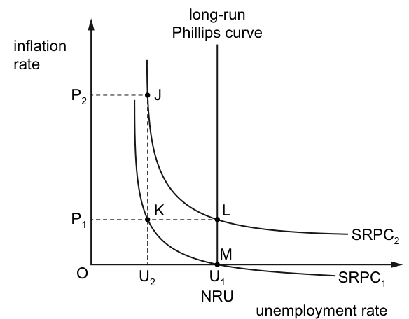
If the government introduces a fiscal stimulus to reduce unemployment, monetarists predict that there will be a series of movements before long-run equilibrium is restored.
Which set of movements illustrates this prediction?
Options
A J to K to L
B L to K to J
C M to K to J
D M to K to L
Working
The economy starts at equilibrium point M, where unemployment equals the natural rate (U1) and inflation is 0. A fiscal stimulus is expansionary, increasing aggregate demand. In the short run, this reduces unemployment below the natural rate to U2 and raises inflation to P1, represented by a movement along the original short-run Phillips curve (SRPC1) from M to K. Monetarists argue that over time, workers adjust their inflation expectations upwards in response to the higher inflation. This causes the short-run Phillips curve to shift right to SRPC2, as higher expected inflation leads to higher wage demands and higher costs for firms. In the long run, unemployment returns to the natural rate (U1), but inflation remains at P1, represented by a movement from K to L on the new SRPC2. This sequence is M to K to L.
Answer
D
D
Background Concept
The Phillips curve illustrates the short-run inverse relationship between the rate of inflation and the rate of unemployment. Monetarist (new classical) economists extend this model with the expectations-augmented Phillips curve, which distinguishes between short-run and long-run relationships. The long-run Phillips curve (LRPC) is vertical at the natural rate of unemployment (NRU): the rate of unemployment that exists when the labour market is in equilibrium, with no cyclical unemployment, only structural and frictional unemployment. Monetarists argue there is no long-run trade-off between inflation and unemployment: any attempt to reduce unemployment below the NRU using expansionary demand-side policy will only lead to permanently higher inflation, with unemployment eventually returning to the NRU.
In the short run, a downward-sloping short-run Phillips curve (SRPC) shows the trade-off: higher inflation is associated with lower unemployment, and vice versa. The position of the SRPC depends on expected inflation. If expected inflation rises, the SRPC shifts upwards (to the right), meaning that for any given level of unemployment, the actual inflation rate is higher. This shift occurs because workers adjust their wage demands to reflect higher expected inflation, increasing firms' costs and pushing actual inflation up.
Understanding the Question
This 1-mark multiple-choice question asks you to identify the sequence of movements on a Phillips curve diagram that matches the monetarist prediction of the effects of a fiscal stimulus (expansionary fiscal policy) aimed at reducing unemployment. The diagram shows the original equilibrium at point M, where unemployment is at the NRU (U1) and inflation is 0 (no inflation). The question requires you to apply the monetarist model to trace the short-run and long-run adjustments following the policy.
Approach
To answer this, first recall the core monetarist prediction for expansionary demand policy:
- Short-run effect: The fiscal stimulus increases aggregate demand, raising output and reducing unemployment below the NRU, while pushing up inflation. This is a movement along the existing short-run Phillips curve.
- Long-run adjustment: Workers observe the higher inflation and revise their inflation expectations upwards. This causes the short-run Phillips curve to shift right. As wage demands rise to match higher expected inflation, firms' costs increase, aggregate supply shifts left, output falls back to potential, and unemployment returns to the NRU. Inflation is now permanently higher than before.
Next, map this sequence to the labelled points on the diagram:
- Original equilibrium: M (U1, 0% inflation)
- Short-run effect of stimulus: movement to a point with lower unemployment (U2) and higher inflation (P1) → this is point K on SRPC1
- Long-run adjustment after expectations shift: movement back to NRU (U1) at the new higher inflation rate (P1) → this is point L on SRPC2
Step-by-Step Reasoning
- The economy starts at point M, the original long-run equilibrium: unemployment equals the NRU (U1), and inflation is 0. This is the baseline before the policy is introduced.
- The government introduces a fiscal stimulus (e.g., increased government spending or tax cuts), which is expansionary. This raises aggregate demand, so firms increase output and hire more workers. Unemployment falls from U1 to U2, while the higher demand pushes up the inflation rate to P1. This is a movement along the original short-run Phillips curve (SRPC1) from M to K, as there is a short-run trade-off between lower unemployment and higher inflation.
- Over time, workers notice that inflation has risen to P1 and adjust their inflation expectations upwards. They will demand higher nominal wages to preserve their real wages, which increases firms' production costs. Higher costs cause the short-run aggregate supply curve to shift left, reducing output back to its potential level. As a result, unemployment rises back to the NRU (U1), but inflation remains at P1.
- This adjustment is represented by a rightward shift of the short-run Phillips curve from SRPC1 to SRPC2, and a movement from point K to point L. Point L lies on both the new SRPC2 and the long-run Phillips curve, confirming it is the new long-run equilibrium: unemployment is back at the NRU, but inflation is permanently higher at P1.
- The full sequence is therefore M → K → L, which corresponds to option D.
The other options are incorrect:
- Option A (J to K to L) starts at J, which is not the original equilibrium (original equilibrium is M, with 0 inflation).
- Option B (L to K to J) describes a deflationary policy reducing inflation, the opposite of a fiscal stimulus.
- Option C (M to K to J) ends at J, where unemployment is still below the NRU (U2) and inflation is P2. This would only occur if the government continued to stimulate the economy to keep unemployment below the NRU, but this is not a long-run equilibrium, as the SRPC would keep shifting right and inflation would rise further. The question asks for the sequence until long-run equilibrium is restored, which requires unemployment to return to the NRU.
Key Takeaways
- Monetarists argue there is no long-run trade-off between inflation and unemployment: the LRPC is vertical at the NRU.
- Expansionary demand-side policy can reduce unemployment below the NRU only in the short run, at the cost of higher inflation.
- In the long run, inflation expectations adjust, the SRPC shifts right, and unemployment returns to the NRU with permanently higher inflation.
- When tracing movements on the Phillips curve, distinguish between movements along a curve (caused by changes in aggregate demand) and shifts of the curve (caused by changes in expected inflation).
Common Mistakes
- Confusing the monetarist view with a Keynesian view that accepts a permanent long-run trade-off between inflation and unemployment. Monetarists argue the trade-off only exists in the short run.
- Forgetting that the original equilibrium is at point M (0 inflation, NRU), so any sequence starting at J or L is invalid.
- Selecting option C (M to K to J), which incorrectly assumes the government can keep unemployment below the NRU permanently. Monetarists argue this is impossible, as rising inflation expectations will shift the SRPC right, pushing unemployment back to the NRU.
- Mixing up movements along the SRPC (short-run demand changes) with shifts of the SRPC (changes in expected inflation).
Things to Be Careful About
- Always identify the original equilibrium first: in this question, it is point M, as the question states the economy is originally in equilibrium with no inflation, which matches M's position at 0 inflation and U1 (NRU).
- Long-run equilibrium must lie on the LRPC, so any endpoint with unemployment not equal to U1 (like J, which is at U2) cannot be the long-run equilibrium.
- The short-run effect of expansionary policy is a movement along the existing SRPC, not a shift. The shift only occurs later, when inflation expectations adjust.
- The sequence must end at a point on the LRPC, as that is the long-run equilibrium for monetarists.
An economy has a sudden increase in inflation caused by a large rise in energy prices. It also enters a recession with rising unemployment.
A decrease in which policy variable is most likely to reduce the impact of the recession without increasing the price level further?
Options
A direct taxation
B government spending
C indirect taxation
D interest rate
Reasoning
The economy is experiencing stagflation: a rise in the price level (inflation) caused by a supply-side shock (higher energy prices) together with a recession (falling output and rising unemployment). To reduce the impact of the recession, we need to increase aggregate demand or aggregate supply. However, increasing aggregate demand would further raise the price level, worsening inflation. Therefore, the policy must increase aggregate supply, which can lower both the price level and raise output.
A decrease in indirect taxation reduces firms' costs, shifting the short-run aggregate supply (SRAS) curve to the right. This reduces the price level and increases real output, directly addressing both problems.
Decreasing direct taxation (A) or increasing government spending (B) are demand-side policies that would shift aggregate demand to the right, raising output but also increasing the price level, worsening inflation. Decreasing the interest rate (D) is an expansionary monetary policy that also stimulates aggregate demand, with the same effect.
Thus, only a decrease in indirect taxation (C) can reduce the impact of the recession without increasing the price level further.
Answer
C
C
Background Concept
Stagflation occurs when an economy experiences both high inflation and high unemployment simultaneously. This is typically caused by a supply-side shock, such as a sharp rise in energy prices, which increases production costs and shifts the short-run aggregate supply (SRAS) curve leftward. The leftward shift of SRAS reduces real output (causing recession) and raises the price level (causing inflation). The AD-AS model is the standard tool for analysing such scenarios.
Demand-side policies (fiscal policy using taxes or government spending, and monetary policy using interest rates) affect aggregate demand (AD). Supply-side policies affect aggregate supply (AS). The policy challenge in stagflation is that expansionary demand-side policies would increase AD, raising output but also pushing the price level even higher, worsening inflation. Contractionary demand-side policies would reduce inflation but deepen the recession. Therefore, supply-side policies that shift SRAS rightward are the only way to simultaneously reduce both inflation and unemployment.
Understanding the Question
The question describes an economy that has a sudden increase in inflation due to a large rise in energy prices (cost-push inflation) and also enters a recession with rising unemployment. We are asked to identify which policy variable, if decreased, is most likely to reduce the impact of the recession without increasing the price level further. The key constraint is “without increasing the price level further”. This means the policy must not be inflationary. The options are four policy variables: direct taxation, government spending, indirect taxation, and interest rate. We need to determine the effect of a decrease in each on both output and the price level, and choose the one that boosts output without raising the price level.
Approach
We will evaluate each option in turn, using the AD-AS framework. For each, we consider the direction of a decrease and its likely effect on aggregate demand (AD) and/or aggregate supply (AS). Then we assess whether the combination of changes in output and price level meets the requirement of reducing recession impact (higher output) without increasing the price level. The only option that can achieve this is the one that shifts SRAS to the right. All other options either shift AD (which trades off higher output for higher inflation) or are contractionary.
Step-by-Step Reasoning
-
Option A: Decrease direct taxation – Direct taxes (e.g., income tax) affect disposable income. A decrease in direct taxation leaves households with more disposable income, which increases consumption expenditure. This is a demand-side policy: consumption is a component of aggregate demand. AD shifts rightward. In the AD-AS diagram, the rightward shift of AD raises both real output and the price level. While the recession is alleviated (output rises), the price level rises further, worsening inflation. This violates the condition “without increasing the price level further”. Therefore, option A is not suitable.
-
Option B: Decrease government spending – Government spending is a component of aggregate demand. A decrease in government spending reduces AD, shifting AD leftward. This would reduce both output and the price level. Reducing output exacerbates the recession, so this option does not reduce the impact of the recession; it makes it worse. Therefore, option B is not suitable.
Note: The question asks for a “decrease in which policy variable”. For government spending, a decrease is contractionary, so it is immediately counterproductive. Some students might mistakenly think a decrease in government spending is expansionary; it is not.
-
Option C: Decrease indirect taxation – Indirect taxes (e.g., VAT, sales tax) are levied on goods and services. A decrease in indirect taxation reduces the cost of production for firms (or lowers the price of goods, effectively reducing costs). This is a supply-side policy: it shifts the SRAS curve to the right. In the AD-AS diagram, a rightward shift of SRAS leads to an increase in real output and a decrease in the price level. Thus, the recession is mitigated (output rises) and inflation is reduced (price level falls). This meets the requirement exactly: the recession impact is reduced, and the price level does not increase further; it actually decreases. Therefore, option C is correct.
-
Option D: Decrease interest rate – The interest rate is a monetary policy tool. A decrease in the interest rate makes borrowing cheaper, encouraging investment and consumption spending. This increases aggregate demand (AD shifts right). Similar to option A, this raises both output and the price level. While the recession is alleviated, inflation worsens. Hence, option D does not satisfy the condition.
Thus, only a decrease in indirect taxation (option C) can simultaneously reduce the impact of the recession (by increasing output) and avoid raising the price level (by actually lowering it).
Key Takeaways
- Stagflation (cost-push inflation plus recession) creates a policy dilemma: demand-side policies that boost output tend to worsen inflation, and those that reduce inflation deepen the recession.
- Supply-side policies that reduce production costs (e.g., cuts in indirect taxes, deregulation, or productivity improvements) can shift SRAS rightward, addressing both problems simultaneously.
- When evaluating policy options, always consider the direction of the change (increase or decrease) and its effect on AD and/or AS.
- The AD-AS model is essential for analysing the impact of macroeconomic policies on output and the price level.
Common Mistakes
- Assuming all tax cuts are expansionary: Direct tax cuts boost AD; indirect tax cuts boost AS. Students often confuse the two.
- Misinterpreting the direction of policy: For government spending, a decrease is contractionary, not expansionary. Some students might think a decrease in government spending is intended to stimulate the economy, but it is the opposite.
- Ignoring the inflation constraint: The question explicitly says “without increasing the price level further”. Many students choose direct tax cuts or interest rate cuts because they are standard recession-fighting tools, but they fail to check the inflation effect.
- Not considering the supply side: Students may only think in terms of demand management and forget that supply-side policies are available.
Things to Be Careful About
- Read the question precisely: “decrease in which policy variable” – so we are considering a decrease, not an increase. For government spending, a decrease is contractionary.
- For indirect taxation, a decrease is a reduction in the tax rate, not an increase. The effect is to lower costs, shifting SRAS right.
- The price level: the question asks “without increasing the price level further”. A policy that reduces the price level is even better, but at minimum it must not raise it. Only option C achieves a fall in the price level.
- In the AD-AS model, always distinguish between shifts of AD and shifts of AS. This is a common source of confusion.
What is not a threat to globalisation?
Options
A rising fear of losing jobs to immigrant workers
B rising political tensions among major economies of the world
C stronger trade unions in industries producing substitutes of imports
D withdrawal of government support for inefficient industries
Answer
Globalisation is the increasing integration of economies through trade, investment, and movement of labour. Threats to globalisation are factors that reduce this integration, such as protectionist sentiment, political conflicts, and lobbying for trade barriers.
- A: Rising fear of losing jobs to immigrant workers can lead to anti-immigration policies and protectionism, which threaten globalisation.
- B: Rising political tensions among major economies can disrupt trade agreements and cooperation, threatening globalisation.
- C: Stronger trade unions in import-competing industries may push for tariffs or quotas, threatening globalisation.
- D: Withdrawal of government support for inefficient industries reduces subsidies and protection, forcing industries to become more competitive or exit. This aligns with free trade principles and does not threaten globalisation; it may even promote it by reducing distortions.
Therefore, the correct answer is D.
D
Background Concept
Globalisation refers to the growing interdependence of economies worldwide through cross-border trade, investment, and the movement of labour and technology. It is driven by reductions in trade barriers, improved transport and communication, and the spread of multinational enterprises. Threats to globalisation are developments that reverse or slow this integration, such as protectionism, nationalism, conflict, and policies that hinder the free flow of goods, services, capital, or labour.
Understanding the Question
The question asks: "What is not a threat to globalisation?" It provides four options, and the task is to identify the one that does NOT hinder globalisation. This requires understanding what each option implies and whether it would reduce economic integration.
Approach
Evaluate each option in turn, considering whether it would likely lead to reduced trade, investment, or labour mobility, or whether it might actually support globalisation. The correct answer is the one that does not pose a threat, or even promotes globalisation.
Step-by-Step Reasoning
- Option A: Rising fear of losing jobs to immigrant workers. This can lead to calls for stricter immigration controls and anti-immigration policies. Such policies reduce labour mobility, which is a component of globalisation. It can also fuel protectionist trade policies. Therefore, it is a threat.
- Option B: Rising political tensions among major economies. Political tensions can lead to trade disputes, sanctions, and reduced cooperation in international organisations. This threatens the stability needed for globalisation and can lead to fragmentation. Therefore, it is a threat.
- Option C: Stronger trade unions in industries producing substitutes of imports. These unions represent workers in import-competing industries. They may lobby for tariffs, quotas, or other protectionist measures to shield their jobs from foreign competition. Such protectionism reduces trade and thus threatens globalisation. Therefore, it is a threat.
- Option D: Withdrawal of government support for inefficient industries. This means the government stops providing subsidies, tax breaks, or other forms of assistance to uncompetitive firms. Without support, these industries may shrink or close, allowing resources to move to more efficient uses. This is consistent with free trade and open markets, as it reduces market distortions and encourages competition. It does not threaten globalisation; it may actually enhance it by making the economy more open and efficient. Therefore, it is not a threat.
Key Takeaways
- Globalisation is threatened by protectionism, nationalism, conflict, and policies that restrict trade, investment, or migration.
- Policies that reduce government intervention and support for inefficient industries tend to promote globalisation by aligning with comparative advantage and free trade.
- When evaluating threats, consider whether the factor directly reduces cross-border economic integration.
Common Mistakes
- Assuming that any change that harms domestic industries is a threat to globalisation. In fact, the withdrawal of support for inefficient industries may harm those industries but does not reduce global trade; it may even increase it.
- Confusing protectionist policies (threats) with policies that remove trade barriers (promoters of globalisation).
- Not reading the question carefully: "not a threat" means the odd one out.
Things to Be Careful About
- Distinguish between threats to globalisation and threats to specific industries. The question is about globalisation as a whole.
- Recognise that political tensions and trade union lobbying are typical threats, while government withdrawal of support for inefficient industries is a pro-market reform that often accompanies globalisation.
Singapore has one of the highest population densities in the world. It discourages car use through a high tax on second cars.
Which additional policy would help to relieve road congestion in the short run?
Options
A limiting the total number of car licences issued
B encouraging restrictions on the size of families
C improving infrastructure by building new roads
D replacing diesel cars by electric cars
Answer
Limiting the total number of car licences issued (Option A) directly reduces the number of cars on the road, thereby relieving congestion in the short run. The existing high tax on second cars already discourages ownership but does not cap the total number. Option A is a quantity restriction that immediately limits the vehicle stock. Options B, C and D take longer to have an effect: encouraging restrictions on family size is a long-term demographic policy; improving infrastructure by building new roads takes time to plan and construct; replacing diesel cars with electric cars does not reduce the number of cars, only changes their type, and would not reduce congestion in the short run.
A
Background Concept
Congestion is a negative externality of road use — each driver imposes time costs on others. The socially optimal number of cars is lower than the private equilibrium. Policies to correct this include taxes (the existing tax on second cars), quantity restrictions (licence caps), subsidies for alternatives, and infrastructure investment. The key distinction tested here is between policies that work in the short run (immediate effect) and those that require time.
Understanding the Question
The question asks which additional policy would help relieve road congestion in the short run. Singapore already taxes second cars heavily. The answer must be a policy that can reduce the number of cars on the road almost immediately. The term "short run" is crucial — any policy that takes years to implement or change behaviour is not correct.
Approach
Evaluate each option's time frame:
- A: a direct quantity restriction — can be imposed immediately, reducing the number of licences and thus cars.
- B: family size restrictions — affects birth rates, takes decades to change population.
- C: building new roads — requires planning, land acquisition, construction; years.
- D: replacing diesel cars with electric — does not reduce the number of cars; even if hastened, the switch takes time and does not lower congestion.
Only A has a short-run impact.
Step-by-Step Reasoning
- Option A: Limiting the total number of car licences issued would directly cap the number of cars allowed. Since Singapore already has a system of licences (Certificate of Entitlement), reducing the quota would immediately reduce the number of new cars entering the road, and over time the total stock would fall. This is effective in the short run because the restriction takes effect as soon as the quota is announced and enforced.
- Option B: Encouraging restrictions on family size would affect population growth, which influences overall demand for transport, but this takes generations to have any noticeable effect on congestion. Not short run.
- Option C: Improving infrastructure by building new roads increases road capacity, which can reduce congestion in the long run, but construction takes years. In the short run, it may even worsen congestion due to construction activity. Not short run.
- Option D: Replacing diesel cars with electric cars does not reduce the number of vehicles. Electric cars still take up road space and cause congestion. This policy addresses emissions, not congestion. Not short run.
Thus, only A qualifies.
Key Takeaways
- Time horizon is critical when evaluating policy effectiveness. "Short run" means immediate or very quick impact.
- Quantity restrictions (licences, quotas) are effective in the short run because they directly limit the source of the problem.
- Infrastructure investment is a long-run solution; it does not relieve congestion immediately.
- Policies must be matched to the specific problem: congestion vs. pollution.
Common Mistakes
- Choosing C (building roads) because it seems like a standard solution to congestion, without considering the short-run constraint.
- Not noticing the existing tax on second cars; the question asks for an additional policy, not a substitute.
- Confusing short-run with long-run effects.
Things to Be Careful About
- Read the question carefully: "in the short run" is the key qualifier.
- Understand that reducing the number of cars is necessary to relieve congestion; improving efficiency (electric cars) does not reduce numbers.
- Be aware of the Singapore context: the Certificate of Entitlement system is a real-world example of a licence limitation.
What is not an example of an expenditure-reducing policy?
Options
A a decrease in government spending
B a depreciation of the exchange rate
C an increase in direct taxes
D an increase in interest rates
Answer
Expenditure-reducing policies aim to lower aggregate demand to correct a current account deficit. Decreases in government spending (A) and increases in direct taxes (C) are contractionary fiscal policy, and an increase in interest rates (D) is contractionary monetary policy; all three reduce aggregate demand. A depreciation of the exchange rate (B) makes exports cheaper and imports dearer, switching expenditure from foreign to domestic goods without necessarily reducing total expenditure; it is an expenditure-switching policy. Therefore, B is not an expenditure-reducing policy.
B
Background Concept
Expenditure-reducing policies are macroeconomic policies designed to reduce the level of aggregate demand in an economy. They are typically used to correct a current account deficit by lowering imports (which are a function of income) and also reducing inflationary pressure. The main instruments are contractionary fiscal policy (reducing government spending or increasing taxes) and contractionary monetary policy (increasing interest rates).
Expenditure-switching policies, by contrast, aim to shift the composition of spending between domestic and foreign goods, without necessarily changing the total level of expenditure. The most prominent example is exchange rate depreciation (or devaluation under a fixed system), which makes exports cheaper relative to foreign goods and imports more expensive, encouraging a switch from imports to domestically produced goods.
Understanding the Question
The question asks which of the four listed policies is NOT an example of an expenditure-reducing policy. To answer correctly, you must know what constitutes expenditure-reducing and then classify each option. The correct answer is the one that is instead expenditure-switching.
Approach
First, recall the definition of expenditure-reducing policies: those that cut aggregate demand. Then evaluate each option:
- A: a decrease in government spending -> cuts AD via the fiscal channel -> expenditure-reducing.
- B: a depreciation of the exchange rate -> does not cut AD directly; it reallocates spending -> expenditure-switching.
- C: an increase in direct taxes -> reduces disposable income, cuts consumption -> expenditure-reducing.
- D: an increase in interest rates -> raises cost of borrowing, reduces investment and consumption -> expenditure-reducing.
Thus, B is the odd one out.
Step-by-Step Reasoning
-
Define expenditure-reducing policy: Any macroeconomic policy that reduces aggregate demand to lower the level of imports (since imports are positively related to national income) or to free up resources for export. Typically, this includes contractionary fiscal and monetary policies.
-
Evaluate option A: A decrease in government spending directly reduces G in the aggregate demand equation (AD = C + I + G + X - M). This lowers overall expenditure in the economy, reducing import demand. It is clearly expenditure-reducing.
-
Evaluate option B: A depreciation of the exchange rate means the domestic currency becomes weaker relative to foreign currencies. This makes exports cheaper abroad and imports more expensive at home. The effect is to increase exports and reduce imports, improving the current account. However, total aggregate demand may not necessarily fall; in fact, if net exports rise, AD could increase. The policy works by changing the relative prices of domestic and foreign goods, thereby switching expenditure from imports to domestic goods. It is expenditure-switching, not expenditure-reducing.
-
Evaluate option C: An increase in direct taxes (e.g., income tax) reduces households' disposable income. With lower income, consumption (C) falls, which reduces AD. This is contractionary fiscal policy and hence expenditure-reducing.
-
Evaluate option D: An increase in interest rates raises the cost of borrowing and provides a higher return on saving. This discourages consumption (especially of durable goods bought on credit) and investment (I), reducing AD. This is contractionary monetary policy, thus expenditure-reducing.
-
Conclusion: Options A, C, and D are all expenditure-reducing; option B is expenditure-switching. Therefore, B is the correct answer.
Key Takeaways
- Expenditure-reducing policies directly lower aggregate demand; they include contractionary fiscal and monetary policy.
- Expenditure-switching policies change the relative attractiveness of domestic versus foreign goods, primarily through exchange rate changes.
- Knowing the distinction is crucial for analysing balance of payments adjustment mechanisms.
Common Mistakes
- Confusing expenditure-reducing with expenditure-switching: some students think depreciation reduces expenditure because it makes imports more expensive, but it does not necessarily reduce total spending; it changes its composition.
- Not recognising that both fiscal and monetary contraction can serve as expenditure-reducing policies.
- Thinking that a decrease in government spending (A) is not expenditure-reducing because it might be aimed at other objectives; but it is contractionary fiscal policy regardless of the objective.
Things to Be Careful About
- The question asks for 'not an example', so ensure you are identifying the exception.
- Remember that expenditure-reducing policies work through the income channel (reducing national income and thus imports), while expenditure-switching works through relative prices.
- In some contexts, a depreciation might eventually have a small contractionary effect on AD if the economy is import-dependent and the spending switch is incomplete, but the standard classification treats it as expenditure-switching.
What does the J-curve effect show?
Options
A A successful currency depreciation requires the sum of the import and export elasticities of demand to be greater than 1.
B After a currency devaluation, the current account is likely to get worse before it gets better.
C In the short run, the demand for imports and exports tends to be price elastic.
D The value of the terms of trade will affect the success of a currency’s devaluation.
Answer
The J-curve effect shows that after a currency devaluation, the current account is likely to get worse before it gets better. Option B correctly captures this. Option A is the Marshall-Lerner condition, which is a related but distinct concept. Option C is incorrect because in the short run, demand for imports and exports tends to be price inelastic, not elastic. Option D refers to the terms of trade, which is not the focus of the J-curve effect. Therefore, the correct answer is B.
B
B
Background Concept
The J-curve effect is a key concept in international economics that describes the time path of a country's current account balance following a currency devaluation or depreciation. When a currency is devalued, the immediate effect is that the price of imports rises in domestic currency terms, while the price of exports falls in foreign currency terms. However, the quantities of imports and exports do not adjust instantly due to contracts, production lags, and consumer habits. In the short run, the volume of imports remains relatively unchanged, but their value increases, while the volume of exports may not increase immediately. This leads to a worsening of the current account. Over time, as consumers and firms adjust to the new prices, the volume of exports rises and the volume of imports falls, leading to an improvement in the current account. The pattern of initial deterioration followed by improvement resembles the letter J, hence the name.
The J-curve effect is closely related to the Marshall-Lerner condition, which states that a devaluation will improve the current account in the long run if the sum of the price elasticities of demand for exports and imports is greater than one. The J-curve explains why the short-run effect may be opposite to the long-run effect.
Understanding the Question
The question asks: "What does the J-curve effect show?" It is a multiple-choice question with four options. The correct answer is the one that accurately describes the J-curve phenomenon. The question tests whether the candidate understands the temporal pattern of the current account after a devaluation, and can distinguish it from related concepts like the Marshall-Lerner condition, the elasticity of demand, and the terms of trade.
Approach
To answer this question, recall the definition of the J-curve effect. Identify which option directly matches that definition. Then, for each incorrect option, recognize why it describes a different concept or is factually incorrect. This will confirm that the chosen option is indeed correct.
Step-by-Step Reasoning
-
Option A: "A successful currency depreciation requires the sum of the import and export elasticities of demand to be greater than 1." This is the Marshall-Lerner condition, which is a necessary condition for a devaluation to improve the current account in the long run. It does not describe the J-curve effect, which is about the time path of the current account. So A is incorrect.
-
Option B: "After a currency devaluation, the current account is likely to get worse before it gets better." This is exactly the J-curve effect. The initial worsening occurs because the value of imports rises immediately while volumes are slow to adjust. Over time, the current account improves as volumes respond. This option is correct.
-
Option C: "In the short run, the demand for imports and exports tends to be price elastic." This is false. In the short run, demand for imports and exports is generally price inelastic because consumers and firms do not quickly adjust their purchasing patterns. The J-curve effect relies on this short-run inelasticity. If demand were elastic in the short run, the current account would improve immediately. So C is incorrect.
-
Option D: "The value of the terms of trade will affect the success of a currency’s devaluation." The terms of trade (the ratio of export prices to import prices) can change after a devaluation, and this can affect the current account. However, the J-curve effect specifically refers to the time path of the current account, not the role of the terms of trade. While the terms of trade may be relevant, this option does not define the J-curve effect. So D is incorrect.
Thus, the correct answer is B.
Key Takeaways
- The J-curve effect illustrates the short-run deterioration and long-run improvement of the current account after a currency devaluation.
- The Marshall-Lerner condition is a separate concept that specifies the condition for long-run improvement.
- Short-run price inelasticity of demand for imports and exports is crucial for the J-curve pattern.
Common Mistakes
- Confusing the J-curve effect with the Marshall-Lerner condition. Students may think that the J-curve is about the elasticities being greater than one, but it is about the time path.
- Believing that the current account improves immediately after a devaluation. This ignores the time lags in adjustment.
- Thinking that the J-curve applies only to fixed exchange rate systems; it applies to any devaluation or depreciation.
Things to Be Careful About
- Distinguish between short-run and long-run price elasticities. The J-curve relies on the fact that in the short run, demand is inelastic.
- Remember that the J-curve effect is about the current account, not the balance of trade or the terms of trade. The current account includes not only trade in goods and services but also income and transfers, though the J-curve is often discussed in the context of the trade balance.
- In the exam, pay attention to the exact wording of options. Option B uses "worse before it gets better," which is a classic description of the J-curve.
What is the most likely consequence of an increase in the number of multinational companies?
Options
A a decrease in advancements in technology
B a decrease in foreign direct investment
C an increase in exports
D an increase in unemployment
Reasoning
Multinational companies (MNCs) typically establish production facilities in host countries to take advantage of lower costs or access to markets. They often export a significant proportion of their output, so an increase in the number of MNCs is likely to increase the host country's exports.
Options A, B, and D are incorrect because MNCs generally bring advanced technology (so A is false), increase foreign direct investment (so B is false), and create jobs rather than increase unemployment (so D is false).
Answer
C
C
Background Concept
Multinational companies (MNCs) are large firms that operate in multiple countries. They often set up subsidiaries or production facilities abroad. The presence of MNCs in a host economy can have several economic consequences: they bring capital and technology, increase competition, employ local labour, and often export goods to other countries. Increased exports from the host country are a common outcome because MNCs produce goods for global markets.
Understanding the Question
This multiple-choice question asks for the most likely consequence of an increase in the number of MNCs. The options are: a decrease in advancements in technology, a decrease in foreign direct investment, an increase in exports, and an increase in unemployment. The question tests knowledge of the typical effects of MNCs on host countries.
Approach
Evaluate each option in turn against what is known about MNCs:
- MNCs are a vehicle for technology transfer, so they would not decrease technology.
- MNCs themselves are a major source of foreign direct investment (FDI), so more MNCs would increase FDI, not decrease it.
- MNCs often export from the host country, so an increase in MNCs is likely to increase exports.
- MNCs create jobs, so they would reduce unemployment, not increase it.
Step-by-Step Reasoning
- Option A: MNCs bring advanced technology and know-how to host countries, often through training and investment in modern equipment. This would increase technological advancements, not decrease them. So A is incorrect.
- Option B: Foreign direct investment (FDI) occurs when a firm invests directly in facilities in another country. MNCs are the primary agents of FDI. Therefore, an increase in the number of MNCs would lead to more FDI, not less. So B is incorrect.
- Option C: MNCs set up production in host countries to serve both local and international markets. They often export a substantial share of their output to other countries, thereby increasing the host country's export volume. This is a well-documented consequence. So C is correct.
- Option D: MNCs hire local workers, create jobs directly and indirectly through supply chains, and often pay higher wages than local firms. This tends to reduce unemployment, not increase it. So D is incorrect.
Key Takeaways
- MNCs are a significant source of exports for host developing countries.
- MNCs are associated with technology transfer, FDI inflows, and job creation.
- Questions about the consequences of MNCs should be answered by considering the typical economic effects observed in host economies.
Common Mistakes
- Confusing FDI with something else: FDI is the investment made by MNCs, so more MNCs means more FDI.
- Assuming MNCs extract resources without exporting: MNCs often export, so exports increase.
- Thinking MNCs cause unemployment due to competition: while they may displace some local firms, the net effect is usually job creation.
Things to Be Careful About
- Read the question carefully: it asks for the 'most likely' consequence, so even if some MNCs might not increase exports, the general trend is clear.
- Avoid overthinking: the answer is straightforward based on standard economic reasoning about MNCs.
The table shows the GDP and population of four countries.
Which country is most likely to have the lowest standard of living?
| country | GDP US$ billion | population million | |
|---|---|---|---|
| A | Bangladesh | 206.7 | 153.5 |
| B | India | 2989.1 | 1147.9 |
| C | Nigeria | 292.7 | 138.3 |
| D | South Africa | 467.1 | 43.8 |
Options
A Bangladesh
B India
C Nigeria
D South Africa
Working
GDP per capita is calculated as GDP / population.
- Bangladesh: 206.7 / 153.5 = 1.3466 (billions per million) = US$1346.6 per person.
- India: 2989.1 / 1147.9 = 2.6044 = US$2604.4 per person.
- Nigeria: 292.7 / 138.3 = 2.1167 = US$2116.7 per person.
- South Africa: 467.1 / 43.8 = 10.6644 = US$10664.4 per person.
Bangladesh has the lowest GDP per capita.
Answer
A
A
Background Concept
Standard of living is often measured by GDP per capita, which is the total value of goods and services produced in a country divided by its population. A higher GDP per capita generally indicates a higher average income and, assuming similar price levels, a higher material standard of living. However, GDP per capita is a narrow measure and does not capture inequality, non-market activities, or environmental quality, but it is a useful starting point for cross-country comparison.
Understanding the Question
The question provides GDP (in US$ billions) and population (in millions) for four countries: Bangladesh, India, Nigeria, and South Africa. It asks which country is most likely to have the lowest standard of living. The most direct monetary indicator is GDP per capita. Since the data is given in billions and millions, we need to compute GDP per capita consistently to compare.
Approach
- Calculate GDP per capita for each country by dividing GDP (in billions) by population (in millions). This gives GDP per capita in thousands of US$ per person. Alternatively, multiply GDP by 1000 to get millions of US$ and then divide by population (in millions) to get US$ per person.
- Compare the resulting values. The country with the smallest GDP per capita is most likely to have the lowest standard of living.
- Select the corresponding option letter.
Step-by-Step Reasoning
- For Bangladesh: GDP = 206.7 billion, population = 153.5 million. GDP per capita = (206.7 * 1000) / 153.5 = 206700 / 153.5 ≈ 1346.6 US$ per person.
- For India: GDP = 2989.1 billion, population = 1147.9 million. GDP per capita = (2989.1 * 1000) / 1147.9 = 2989100 / 1147.9 ≈ 2604.4 US$ per person.
- For Nigeria: GDP = 292.7 billion, population = 138.3 million. GDP per capita = (292.7 * 1000) / 138.3 = 292700 / 138.3 ≈ 2116.7 US$ per person.
- For South Africa: GDP = 467.1 billion, population = 43.8 million. GDP per capita = (467.1 * 1000) / 43.8 = 467100 / 43.8 ≈ 10664.4 US$ per person.
Comparing: Bangladesh (1346.6) < Nigeria (2116.7) < India (2604.4) < South Africa (10664.4). Thus Bangladesh has the lowest GDP per capita, so it is most likely to have the lowest standard of living.
Key Takeaways
- GDP per capita is a commonly used proxy for standard of living.
- To compare across countries, one must use consistent units (e.g., same currency, adjusted for population).
- Simple arithmetic can answer such questions quickly.
Common Mistakes
- Forgetting to convert units: GDP in billions and population in millions, dividing directly gives a number in thousands; failing to multiply by 1000 leads to an incorrect ratio (e.g., 206.7/153.5 = 1.35, which is not the correct per capita figure in dollars). The correct interpretation is that 1.35 is in thousands of dollars, so $1350.
- Misreading the table: e.g., thinking the largest GDP implies highest standard of living without considering population.
- Not performing the calculation and guessing based on total GDP alone.
Things to Be Careful About
- Always check the units of GDP and population. In this question, GDP is in billions and population in millions, so the quotient is in thousands of US$ per person.
- Ensure that the comparison is on the same metric (GDP per capita) and not on total GDP.
- Remember that GDP per capita is a very rough measure; it does not account for income distribution, cost of living, or non-monetary aspects of well-being.
What will increase the size of a country’s optimum population?
Options
A a rise in the birth rate
B a lowering of the age of retirement
C a rise in the stock of capital available in the country
D a decrease in the productivity of the country’s industries
Answer
The optimum population of a country is the population size that, with the country's existing resources and technology, yields the highest possible output per capita. It is not a fixed number but changes when the resource base or technology changes.
A rise in the stock of capital (option C) increases the country's productive capacity. With more capital per worker, each worker can produce more output, so a larger population can be supported while maintaining or increasing output per capita. This raises the optimum population.
Options A and B (rise in birth rate, lowering retirement age) increase the population but do not increase the resource base, so they would move the actual population away from the optimum or reduce output per capita. Option D (decrease in productivity) reduces output per unit of input, lowering the population that can be supported at maximum per capita output, thus reducing the optimum population.
Therefore, the correct answer is C.
C
Background Concept
The optimum population of a country is the population size at which output per capita (or average living standard) is maximised. It is derived from the production possibilities of the economy: given the stock of natural resources, capital, and technology, there is a population level where the average product of labour is highest. If population is below the optimum, adding more workers raises output per head because fixed resources are underutilised. If population is above the optimum, diminishing returns set in and output per head falls. The optimum population moves when the resource base or technology changes, because the production function shifts upward or downward.
Understanding the Question
The question asks: "What will increase the size of a country’s optimum population?" This tests whether you understand that the optimum population is not the actual population, but a theoretical maximum-efficiency level determined by the country's productive capacity. Each option presents a change, and you must decide which one actually expands the capacity to support a larger population at higher per capita output.
Approach
Recall the definition of optimum population: it shifts when the production possibility frontier (PPF) shifts outward due to more resources or better technology. Evaluate each option against this criterion:
- Options that increase the population without expanding resources do NOT shift the optimum.
- Options that enhance productive capacity (capital, technology, resource discoveries) DO shift the optimum outward.
- Options that reduce productive capacity shift the optimum inward.
Step-by-Step Reasoning
- Option C: A rise in the stock of capital – More capital (machinery, infrastructure, factories) increases the productivity of each worker. The average product of labour curve shifts upward, so the maximum output per capita occurs at a higher population size. Thus the optimum population increases. This is correct.
- Option A: A rise in the birth rate – This increases the actual population, but it does not change the resource base or technology. The new, larger population faces the same capital and natural resources, so output per capita will fall. The optimum population (determined by resources) remains unchanged. The question asks about the size of the optimum, not the actual population.
- Option B: A lowering of the age of retirement – This expands the labour force participation rate (more people of working age), but again does not increase capital or technology. The total population may stay the same if only retirement age changes, but the working-age population rises. However, the optimum population is about total population, not labour force alone. With more workers on the same capital stock, diminishing returns set in faster; the optimum population (if defined by total population) does not increase; if anything, it may decrease due to lower capital per worker. So B does not raise the optimum.
- Option D: A decrease in the productivity of the country’s industries – This is a negative technology shock. It reduces output per worker for any given population. The average product curve shifts downward, so the maximum output per capita occurs at a smaller population. Thus the optimum population decreases.
Hence only C is correct.
Key Takeaways
- Optimum population is a function of resources and technology, not current population size.
- Any factor that increases the productivity of the economy (more capital, better technology, more natural resources) tends to raise the optimum population.
- Demographic changes alone (birth rate, retirement age) do not shift the optimum; they only affect actual population, which may deviate from the optimum.
Common Mistakes
- Confusing optimum population with actual population: many candidates incorrectly think a rise in birth rate increases the optimum, but it only increases the actual population.
- Overlooking the role of capital: a rise in the stock of capital is often mistaken as simply making each worker more productive (which is true) but not always linked to supporting a larger population at maximum efficiency.
- Misinterpreting "lowering of the age of retirement" as increasing the labour force, which some think allows more people to be supported – but it doesn't increase the capital stock, so it reduces capital per worker and output per capita.
Things to Be Careful About
- The question asks about the "size of the optimum population", so be sure to focus on changes that shift the production possibilities, not changes that alter the current population.
- Read each option carefully: option B is tricky because it affects the age structure but not total population or resources.
- Remember that optimum population is a static concept given current resources; it changes only when those resources change.
Answer
Therefore, the correct answer is C.
The table shows the values of the Gini coefficient for some countries in a given year.
| Gini coefficient | |
|---|---|
| Namibia | 74.3 |
| Zambia | 50.4 |
| France | 32.7 |
| Denmark | 24.7 |
Using this information, which statement is correct?
Options
A Income is distributed more equally in Denmark than France.
B Income is distributed more equally in Namibia than Zambia.
C Income per capita is higher in Zambia than Namibia.
D There are proportionally more people below the poverty line in Zambia than France.
Reasoning
The Gini coefficient measures income inequality within a country, where a value of 0 represents perfect equality and 100 represents perfect inequality. A lower Gini coefficient indicates a more equal distribution of income.
From the table:
- Denmark: 24.7
- France: 32.7
- Zambia: 50.4
- Namibia: 74.3
Since Denmark (24.7) has a lower Gini coefficient than France (32.7), income is distributed more equally in Denmark than in France. This matches statement A.
Statement B is incorrect because Namibia (74.3) has a higher Gini coefficient than Zambia (50.4), indicating less equal distribution.
Statement C is incorrect because the Gini coefficient does not provide information about income per capita.
Statement D is incorrect because the Gini coefficient does not directly measure the proportion of people below the poverty line; it measures overall inequality.
Answer
A
A
Background Concept
The Gini coefficient is a statistical measure of income inequality within a country or region. It ranges from 0 (perfect equality, where everyone has the same income) to 1 (or 100, if expressed as a percentage) representing perfect inequality (one person has all the income). In practice, values are typically between 0.25 and 0.70 for most countries. The coefficient is derived from the Lorenz curve, which plots the cumulative percentage of income against the cumulative percentage of households. The Gini coefficient is the ratio of the area between the Lorenz curve and the line of perfect equality to the total area under the line of perfect equality.
Understanding the Question
The question provides a table with Gini coefficients for four countries: Namibia (74.3), Zambia (50.4), France (32.7), and Denmark (24.7). It asks which of four statements is correct based on this information. The statements involve comparisons of income equality, income per capita, and poverty rates. The correct interpretation requires understanding that a lower Gini coefficient means more equal income distribution. The question tests the ability to read and compare numbers and to know what the Gini coefficient does and does not indicate.
Approach
First, recall the meaning of the Gini coefficient: higher values indicate more inequality; lower values indicate more equality. Then compare the pairs mentioned in the options:
- Option A: Denmark vs France. Denmark 24.7 < France 32.7, so more equal in Denmark. This is correct.
- Option B: Namibia vs Zambia. Namibia 74.3 > Zambia 50.4, so less equal in Namibia, not more equal. So B is false.
- Option C: Income per capita is not measured by the Gini coefficient. The table does not provide any information about income per capita. Therefore, C cannot be concluded.
- Option D: The proportion of people below the poverty line is not directly given by the Gini coefficient. While higher inequality can be associated with higher poverty, the Gini coefficient alone does not measure the poverty rate. So D is not necessarily correct.
Thus, the only correct statement is A.
Step-by-Step Reasoning
- The Gini coefficient is a measure of income inequality. A lower value means more equal distribution.
- Compare the values for Denmark and France: Denmark has 24.7, France has 32.7. Since 24.7 < 32.7, income is distributed more equally in Denmark. This supports option A.
- Compare Namibia and Zambia: Namibia 74.3, Zambia 50.4. Since 74.3 > 50.4, income is distributed more equally in Zambia, not Namibia. So option B is false.
- The Gini coefficient does not provide information about income per capita. For example, a country could have high inequality but high average income, or low inequality but low average income. Therefore, option C cannot be inferred from the table.
- The proportion of people below the poverty line is a different concept. The Gini coefficient measures inequality, not absolute poverty. While there is often a correlation, it is not a direct measure. Therefore, option D is not necessarily true based on the Gini coefficient alone.
- Hence, the correct answer is A.
Key Takeaways
- The Gini coefficient is a measure of income inequality, not income level or poverty rate.
- A lower Gini coefficient indicates more equal distribution.
- When comparing two countries, the one with the lower Gini coefficient has more equal income distribution.
- Be careful not to confuse inequality with income per capita or poverty.
Common Mistakes
- Thinking that a higher Gini coefficient means better income distribution (common confusion).
- Assuming that the Gini coefficient directly indicates poverty rates or average income.
- Misreading the table and comparing the wrong countries.
Things to Be Careful About
- The scale: the Gini coefficient can be reported as a decimal (0 to 1) or as a percentage (0 to 100). In this table, it is given as a number (likely out of 100). But the interpretation is the same: lower = more equal.
- Do not make unwarranted inferences: the Gini coefficient only measures inequality, not other aspects of economic well-being.
- Always read the table carefully and compare the correct pairs.
Your score so far
Answer a question to start scoring
Your marks add up here as you work through the paper.