Physics 9702/33 — October/November 2025

Cambridge AS Level · Advanced Practical Skills · worked solutions for every part, with the mark scheme

questions

marks

120

minutes

Topics Manipulation, Measurement and Observation · Presentation of Data and Observations · Analysis, Conclusions and Evaluation

Q1MediumManipulation, Measurement and ObservationPresentation of Data and ObservationsAnalysis, Conclusions and Evaluation

In this experiment, you will investigate the oscillations of a pendulum on a board.

(a)

• Fix the string of the pendulum onto the nail using some of the adhesive putty, as shown in Fig. 1.1.

Fig. 1.1

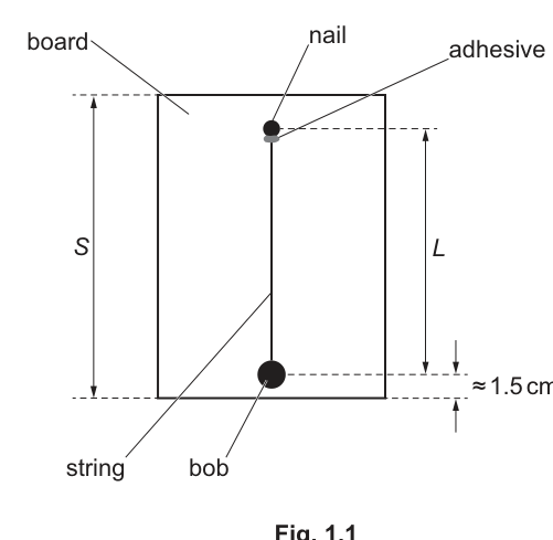
• The distance between the two edges of the board is $S$ , as shown in Fig. 1.1.

The length $L$ of the pendulum is the distance between the centre of the nail and the centre of the bob.

Adjust the length of the pendulum by wrapping the string around the nail so that the centre of the bob is approximately $1.5\text{ cm}$ from the edge of the board.

• Measure and record $S$ and $L$ .

$S$ = ______ $\text{cm}$
$L$ = ______ $\text{cm}$

1M Similar

DifficultyEasy

Worked solution

Answer

(Example readings, to the nearest $0.1\ \text{cm}$ )

$S = 35.0\ \text{cm}$

$L = 33.5\ \text{cm}$

Final answer

S = 35.0 cm, L = 33.5 cm (example)

Detailed explanation

Background Concept

In Paper 3, marks for measurements are awarded for:

measuring the correct quantity (correct reference points)
using an appropriate instrument (typically a mm-scale ruler)
recording to a sensible precision with units.

Here:

$S$ is the distance between the two edges of the board.
$L$ is the length of the pendulum measured from the centre of the nail to the centre of the bob.

Understanding the Question

You are told to set the pendulum so that the bob is about $1.5\ \text{cm}$ from the board edge, then measure and record $S$ and $L$ .

So you must:

measure $S$ between the edges shown,
measure $L$ using centre-to-centre points (not from the string end or bob edge),
record both with units (cm) and appropriate precision.

Approach

Use a ruler placed along the board.
For each length, align the ruler carefully and read at eye level to avoid parallax.
Record in cm to the nearest $0.1\ \text{cm}$ (typical for a mm ruler).

Step-by-Step Reasoning

Measure $S$ :
- Place the ruler so its scale runs perpendicular between the two edges.
- Read the separation between the edges.
- Record as $S = \dots\ \text{cm}$ to $0.1\ \text{cm}$ .
Measure $L$ :
- Identify the centre of the nail head (pivot point) and the centre of the bob.
- Measure the straight-line distance between these two centres.
- Record as $L = \dots\ \text{cm}$ to $0.1\ \text{cm}$ .

(Any values consistent with your apparatus are acceptable; the mark is for correct technique and recording.)

Key Takeaways

Measure between the stated reference points (centre-to-centre for $L$ ).
Record with units and suitable resolution.

Common Mistakes

Measuring $L$ to the edge of the bob instead of its centre.
Omitting units.
Recording with inconsistent precision (e.g. $35\ \text{cm}$ for one value and $33.52\ \text{cm}$ for another using only a ruler).

Things to Be Careful About

Keep the bob about $1.5\ \text{cm}$ from the edge before measuring $L$ (otherwise $L$ changes when you adjust it).
Avoid parallax: eye directly above the scale marking.

Techniques used

measure lengths with a ruler to an appropriate precisionidentify the correct reference points for a length measurementrecord raw readings with units and consistent decimal places

(b)

• Set up the apparatus as shown in Fig. 1.2.

Fig. 1.2

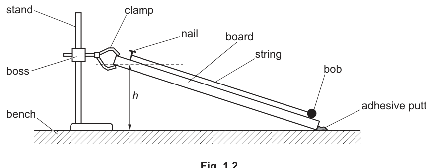
• The distance between the lower edge of the top of the board and the bench is $h$ , as shown in Fig. 1.2.

Adjust the position of the boss so that $h$ is approximately $22\text{ cm}$ .

• Fix the position of the bottom of the board using adhesive putty.

• Measure and record $h$ .

$h$ = ______ $\text{cm}$

• Move the bob to the edge of the board, as shown in Fig. 1.3.

Fig. 1.3

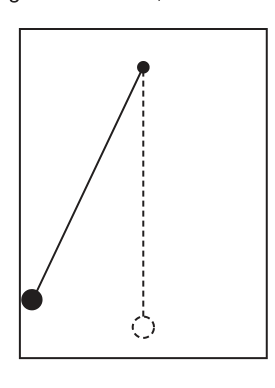
• Release the bob. The bob rolls across the board and the pendulum oscillates.

• Take measurements to determine the period $T$ of the oscillations.

$T$ = ______ $\text{s}$

2M Similar

DifficultyMedium-Easy

Worked solution

Working

(Example reading)

$h = 22.0\ \text{cm}$

Time for $10$ oscillations: $t_{10} = 17.9\ \text{s}$

T = \frac{t_{10}}{10} = \frac{17.9}{10} = 1.79\ \text{s}

Answer

$h = 22.0\ \text{cm}$

$T = 1.79\ \text{s}$

Final answer

h = 22.0 cm, T = 1.79 s (example)

Detailed explanation

Background Concept

The period $T$ of an oscillation is the time for one complete cycle.

Directly timing one oscillation gives a large percentage uncertainty because reaction time (about $0.2\ \text{s}$ ) is a big fraction of $T$ . A standard way to reduce this is:

measure the time for $n$ oscillations ( $n \ge 10$ is common)
then divide by $n$ :

T = \frac{t_n}{n}

Repeating $t_n$ and averaging further improves reliability.

Understanding the Question

You must:

adjust and measure $h$ (vertical distance from the bench to the lower edge of the top of the board),
take measurements to determine the oscillation period $T$ once the bob is released and oscillates.

Approach

Measure $h$ with a ruler, using the exact points stated.
Determine $T$ by timing multiple oscillations (e.g. 10) using a stopwatch, then dividing.
Repeat the timing and take a mean value of $T$ .

Step-by-Step Reasoning

Measuring $h$ :
- Hold the ruler vertically from the bench surface up to the lower edge of the top of the board.
- Record $h$ in cm to the nearest $0.1\ \text{cm}$ .
Measuring $T$ :
- Choose a reference position (often the equilibrium position) and start the stopwatch as the bob passes it in a chosen direction.
- Count $n$ complete oscillations (one oscillation is returning to the same position moving in the same direction).
- Stop the watch after $n$ oscillations and record $t_n$ .
- Calculate $T = t_n/n$ .
- Repeat and average.

Key Takeaways

Period measurements should use multiple oscillations and division.
Repeat readings reduce random error.

Common Mistakes

Timing only one oscillation.
Miscounting oscillations (e.g. counting half-oscillations).
Measuring the wrong height (using the top edge instead of the stated lower edge).

Things to Be Careful About

Keep the oscillations small and consistent each run (large amplitude can slightly change period and increases variability).
Use the same reference point/direction for starting and stopping each timing.

Techniques used

measure a vertical height with a ruler using an appropriate reference pointdetermine a period by timing multiple oscillations and dividingreduce random error by repeating timing measurements and averaging

(c)

Change $h$ in the range $10.0\text{ cm} \leq h \leq 38.0\text{ cm}$ and determine $T$ . Repeat until you have six sets of values of $h$ and $T$ .

Record your results in a table. Include values of $\frac{S}{h}$ and $T^2$ in your table.

8M Similar

DifficultyMedium

Worked solution

Answer

(Example set; your values will depend on your measurements. Use $10.0\ \text{cm} \le h \le 38.0\ \text{cm}$ and obtain 6 sets.)

Take $S = 35.0\ \text{cm}$ .

$h\ /\ \text{cm}$	$T\ /\ \text{s}$	$\dfrac{S}{h}$	$T^2\ /\ \text{s}^2$
10.0	2.66	3.50	7.08
15.0	2.15	2.33	4.62
20.0	1.88	1.75	3.53
25.0	1.69	1.40	2.86
30.0	1.56	1.17	2.43
35.0	1.45	1.00	2.10

Final answer

Six sets of h and T recorded with calculated S/h and T^2 (see table).

Detailed explanation

Background Concept

Good experimental data presentation in Paper 3 typically requires:

a single table containing all results
clear column headings with quantity and unit (units in the heading, not in the body)
raw measurements recorded to appropriate resolution
derived quantities (here $S/h$ and $T^2$ ) calculated correctly and shown to sensible significant figures.

The instruction specifies the range of $h$ and requires 6 sets, so you must vary $h$ across the stated interval to test the relationship reliably.

Understanding the Question

You must:

change $h$ across $10.0\ \text{cm}$ to $38.0\ \text{cm}$ ,
for each $h$ , determine $T$ ,
repeat until you have six pairs $(h, T)$ ,
present results in a table including extra calculated columns $S/h$ and $T^2$ .

So $h$ is the independent variable, $T$ is measured, and $S/h$ and $T^2$ are calculated.

Approach

Choose six values of $h$ spread across the full range (not clustered).
For each $h$ , measure the time for $n$ oscillations (e.g. $n=10$ ) at least twice and average $T$ .
Calculate:

\frac{S}{h}

and

T^2

Record everything in one clearly laid out table.

Step-by-Step Reasoning

Selecting $h$ values:
- Use values from near the ends and in between, e.g. $10, 15, 20, 25, 30, 35\ \text{cm}$ (all within the permitted range).
Measuring $T$ for each $h$ :
- Measure $t_{10}$ for 10 oscillations, then compute $T=t_{10}/10$ .
- Repeat $t_{10}$ and take a mean to reduce random timing error.
Calculating $S/h$ :
- Use your measured $S$ from part (a) and the current $h$ .
- Since both are in cm, $S/h$ is dimensionless (no unit).
Calculating $T^2$ :
- Square your mean period value for each row.
- If $T$ is to 2 d.p., then $T^2$ is usually quoted to 2 d.p. as well.
Tabulation:
- Put units in headings: $h/\text{cm}$ , $T/\text{s}$ , $T^2/\text{s}^2$ .
- Keep consistent decimal places down each column.

Key Takeaways

Use a wide range and enough points (6) to support later graphing.
Derived columns must be calculated and recorded clearly.

Common Mistakes

Missing units in headings (or writing units in every cell).
Fewer than six data sets.
Using an $h$ outside the given range.
Incorrect calculation of $S/h$ (e.g. using $h/S$ ) or $T^2$ .

Things to Be Careful About

Consistent rounding: calculate using full calculator values, then round at the end for the table entry.
If $h$ is recorded to $0.1\ \text{cm}$ , do not give $S/h$ to an unreasonable number of decimal places.

Techniques used

vary the independent variable over the specified rangerecord raw data in a single table with correct headings and unitscalculate derived quantities consistently from measured valueschoose consistent significant figures and decimal places within a column

(d)

(i)

Plot a graph of $T^2$ on the $y$ -axis against $\frac{S}{h}$ on the $x$ -axis.

3M Similar

DifficultyMedium-Easy

Worked solution

Answer

Plot $T^2$ (in $\text{s}^2$ ) on the $y$ -axis against $S/h$ (no unit) on the $x$ -axis, using a suitable scale and plotting all six points accurately.

Final answer

Graph of T^2 (y) against S/h (x) plotted.

Detailed explanation

Background Concept

A good graph in Cambridge practical papers typically earns marks for:

correctly labelled axes (quantity and unit)
sensible, uniform scales that use at least half the graph grid
accurate plotting of points (small, neat crosses) from the table.

Here $S/h$ is dimensionless, so the x-axis has no unit.

Understanding the Question

You are asked to plot:

$y = T^2$ on the vertical axis
$x = S/h$ on the horizontal axis
using your six experimental data points.

Approach

Decide the axis ranges from your smallest and largest values of $S/h$ and $T^2$ .
Choose convenient scales (e.g. 1 big square = 0.2) that avoid awkward jumps.
Label axes as $T^2/\text{s}^2$ and $S/h$ .
Plot all points.

Step-by-Step Reasoning

Find the ranges from the table, e.g. $S/h$ might run from about $1.0$ to $3.5$ .
Set the x-axis to cover slightly beyond this range.
Find $T^2$ range, then set the y-axis similarly.
Mark axis labels:
- x-axis: $S/h$
- y-axis: $T^2 / \text{s}^2$
Plot each point $(S/h,\ T^2)$ with a small cross.

Key Takeaways

Axes must match the required variables and units.
Scales must be linear and make good use of the grid.

Common Mistakes

Swapping axes (plotting $T^2$ on x-axis).
Forgetting the unit on $T^2$ .
Using a scale that uses only a small portion of the graph paper.

Things to Be Careful About

Do not force the graph through the origin unless your data and theory require it.
Ensure each plotted point matches the correct row (avoid transposition errors).

Techniques used

select suitable axis scales that use most of the gridlabel axes with quantity and unitplot experimental points accurately from a results table

(ii)

Draw the straight line of best fit.

1M Similar

(iii)

Determine the gradient and $y$ -intercept of this line.

gradient = ______

$y$ -intercept = ______

2M Similar

DifficultyMedium

Worked solution

Working

Choose two well-separated points on the best-fit line, e.g.
$(S/h,\ T^2) = (3.50,\ 7.05)$ and $(1.00,\ 2.10)$ .

\text{gradient} = \frac{\Delta T^2}{\Delta (S/h)} = \frac{7.05 - 2.10}{3.50 - 1.00} = \frac{4.95}{2.50} = 1.98\ \text{s}^2

Using $T^2 = mx + c$ :

\text{y-intercept} = c = 2.10 - (1.98)(1.00) = 0.12\ \text{s}^2

Answer

gradient $= 1.98\ \text{s}^2$

y-intercept $= 0.12\ \text{s}^2$

Final answer

gradient = 1.98 s^2, y-intercept = 0.12 s^2 (example)

Detailed explanation

Background Concept

For a straight-line graph of $y$ against $x$ :

y = mx + c

Gradient $m$ is:

m = \frac{\Delta y}{\Delta x}

The y-intercept $c$ is the value of $y$ when $x=0$ .

In this experiment the graph is $T^2$ (y) against $S/h$ (x), so:

gradient has the same unit as $T^2$ , i.e. $\text{s}^2$ , because $S/h$ is dimensionless.
y-intercept also has unit $\text{s}^2$ .

Understanding the Question

You must read from your best-fit line:

the gradient
the y-intercept
and write them in the answer spaces.

Approach

Use two points on the best-fit line (not necessarily measured points), widely separated to reduce percentage uncertainty.
Compute $m = \Delta T^2 / \Delta(S/h)$ .
Find the intercept either by reading where the line meets the y-axis ( $x=0$ ) or by substituting one point into $c = y - mx$ .

Step-by-Step Reasoning

diagram-1-diii

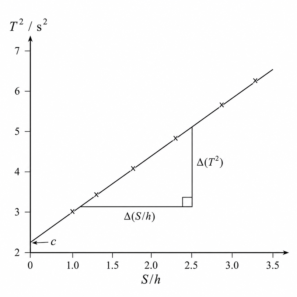
Pick two clear points on the drawn best-fit line. They should be far apart in x to make $\Delta x$ large.
Calculate $\Delta T^2$ and $\Delta(S/h)$ .
Compute the gradient using $m=\Delta y/\Delta x$ .
Determine intercept:
- Either extend the line back to $x=0$ and read $T^2$ .
- Or use $c = y - mx$ with a point on the line.
Quote both with appropriate units ( $\text{s}^2$ ).

Key Takeaways

Always use a large triangle from the best-fit line for gradient.
Intercept is the value at $x=0$ , not at the first data point.

Common Mistakes

Using two plotted data points that are close together (gives a large gradient uncertainty).
Calculating $\Delta x/\Delta y$ instead of $\Delta y/\Delta x$ .
Missing units for gradient and intercept.

Things to Be Careful About

Use points on the line, not the table values unless they lie exactly on the line.
Keep track of which variable is on which axis: here $y=T^2$ and $x=S/h$ .

Techniques used

use a large triangle on the best-fit line to calculate a gradientcalculate gradient as \u0394y/\u0394x with correct unitsdetermine the y-intercept by extrapolating the best-fit line to x = 0

(e)

(i)

It is suggested that the quantities $T$ , $S$ and $h$ are related by the equation

T^2 = A \frac{S}{h} + B

where $A$ and $B$ are constants.

Using your answers in (d)(iii), determine the values of $A$ and $B$ . Give appropriate units.

$A$ = ______

$B$ = ______

2M Similar

(ii)

Theory suggests that

A = \frac{28\pi^2 L}{5g}

where $g$ is the acceleration of free fall.

Use your values in (a) and (e)(i) to determine a value for $g$ . Give an appropriate unit.

$g$ = ______

1M Similar

DifficultyMedium

Worked solution

Working

A = \frac{28\pi^2 L}{5g}\ \Rightarrow\ g = \frac{28\pi^2 L}{5A}

Convert $L$ to metres:

L = 33.5\ \text{cm} = 0.335\ \text{m}

Substitute $A = 1.98\ \text{s}^2$ :

g = \frac{28\pi^2 (0.335)}{5(1.98)} = 9.37\ \text{m s}^{-2}

Answer

$g = 9.37\ \text{m s}^{-2}$

Final answer

g = 9.37 m s^-2 (example)

Detailed explanation

Background Concept

A theoretical model often links an experimentally determined constant (here $A$ ) to physical constants:

A = \frac{28\pi^2 L}{5g}

To find $g$ , rearrange to make $g$ the subject:

g = \frac{28\pi^2 L}{5A}

Unit logic:

$L$ must be in SI units (m)
$A$ has units $\text{s}^2$
So $g$ comes out in $\text{m s}^{-2}$ .

Understanding the Question

You must use:

your measured $L$ from part (a)
your experimental value of $A$ from part (e)(i)
the given theoretical equation

to calculate $g$ and state its unit.

Approach

Rearrange the formula for $g$ .
Convert $L$ from cm to m.
Substitute $L$ and $A$ .
Quote $g$ with unit $\text{m s}^{-2}$ , to a sensible number of significant figures.

Step-by-Step Reasoning

Rearrangement:

A = \frac{28\pi^2 L}{5g} \quad\Rightarrow\quad Ag = \frac{28\pi^2 L}{5} \quad\Rightarrow\quad g = \frac{28\pi^2 L}{5A}

Unit conversion:

L\ (\text{m}) = \frac{L\ (\text{cm})}{100}

Substitution:

put $L$ in m
put $A$ in $\text{s}^2$

Interpretation:

Compare your value with the expected $g \approx 9.81\ \text{m s}^{-2}$ . Small differences are normal due to experimental uncertainties.

Key Takeaways

Always convert lengths to SI units when calculating $g$ .
Experimental constants from graphs can be used to determine physical constants.

Common Mistakes

Using $L$ in cm, giving $g$ that is 100 times too large.
Using $B$ instead of $A$ .
Forgetting the unit of $g$ .

Things to Be Careful About

Use your own $A$ from your own graph; if your gradient has significant uncertainty, your $g$ will too.
Keep enough significant figures during calculation, then round the final answer appropriately.

Techniques used

rearrange an equation to make the target variable the subjectconvert a measured length into SI units before substitutionsubstitute experimental constants into a theoretical expression

Q2MediumManipulation, Measurement and ObservationAnalysis, Conclusions and EvaluationPresentation of Data and Observations

In this experiment, you will investigate the resistance of a light-dependent resistor (LDR) using the light from a light-emitting diode (LED).

(a)

(i)

• Using the LED, set up the circuit shown in Fig. 2.1.

Fig. 2.1

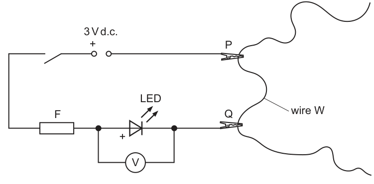
• Ensure that the positive terminal of the power supply and the positive terminal of the LED are connected as shown in Fig. 2.1.

• $P$ and $Q$ are crocodile clips. Position $P$ and $Q$ so that there is approximately $10\text{ cm}$ of wire $W$ between $P$ and $Q$ .

• Close the switch. The LED should light.

• Open the switch.

• Using the LDR and ohmmeter, set up a second circuit as shown in Fig. 2.2.

Fig. 2.2

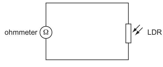
• Arrange the apparatus as shown in Fig. 2.3.

Fig. 2.3

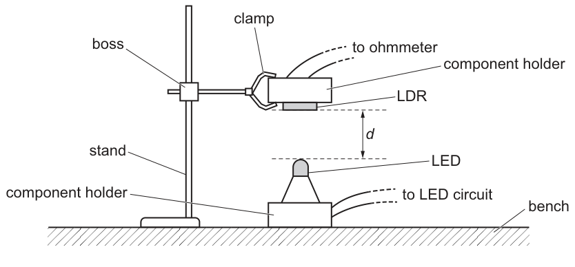
• The distance between the top of the LED and the surface of the LDR is $d$ .

Adjust the position of the LDR so that $d$ is approximately $0.03\text{ m}$ .

• Measure and record $d$ .

$d$ = ______ $\text{m}$

2M Similar

DifficultyMedium-Easy

Worked solution

Answer

Measure $d$ with a ruler/metre rule (vertical distance from top of LED to surface of LDR) and record to the nearest $1\ \text{mm}$ .

Example (typical):

d = 0.030\ \text{m}

Final answer

d ≈ 0.030 m

Detailed explanation

Background Concept

In this experiment, the LED is used as a light source and the LDR changes resistance depending on how much light falls on it. A key control quantity is the separation $d$ between the LED and the LDR: changing $d$ changes the light intensity at the LDR.

A measurement like $d$ must be:

clearly defined (between which two points?),
made along the correct direction (here, vertical),
recorded with an appropriate resolution and unit.

Understanding the Question

You are told to adjust the LDR position so that $d$ is approximately $0.03\ \text{m}$ , then measure and record $d$ . The diagram defines $d$ as the vertical distance between the top of the LED and the surface of the LDR.

So you must:

set the LDR roughly $3\ \text{cm}$ above the LED,
measure that vertical separation,
write the value in metres.

Approach

Use a ruler or metre rule placed as close as possible to the LED–LDR line. Identify the two reference points (top of LED and LDR surface), read the scale at eye level to avoid parallax, and record $d$ with a realistic precision (typically $\pm 1\ \text{mm}$ if using a mm-scale ruler).

Step-by-Step Reasoning

diagram-2a-i

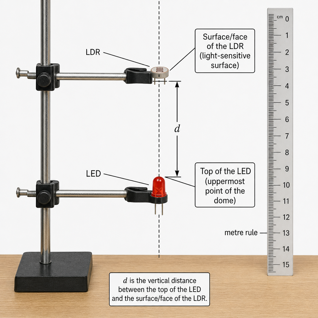
Move the clamp holding the LDR until it is about $3\ \text{cm}$ above the LED.
Place a ruler vertically next to the apparatus.
Read the ruler position at the top of the LED and at the LDR surface.
Subtract to obtain $d$ .

Example:

reading at LDR surface: $8.0\ \text{cm}$
reading at top of LED: $5.0\ \text{cm}$

Then

d = 8.0\ \text{cm} - 5.0\ \text{cm} = 3.0\ \text{cm} = 0.030\ \text{m}

Key Takeaways

Define the measurement clearly using the diagram.
Measure along the required direction (vertical separation).
Record with an appropriate unit and precision.

Common Mistakes

Measuring from the bench to the LDR instead of LED-to-LDR separation.
Measuring to the wrong part of the LED (e.g. base instead of top).
Recording $d$ in cm when the answer line requires metres.
Giving unrealistic precision (e.g. $0.03000\ \text{m}$ with a simple ruler).

Things to Be Careful About

Avoid parallax by reading at eye level.
Keep the ruler close to the LED–LDR line to reduce alignment error.
Ensure you measure the surface of the LDR (light-sensitive face), not the back casing.

Techniques used

set up the circuit with correct polarity and connectionsmeasure a length using a ruler with appropriate precisionrecord a measurement with a unit and sensible significant figures

(ii)

Estimate the percentage uncertainty in your value of $d$ . Show your working.

percentage uncertainty = ______ $\%$

1M Similar

DifficultyMedium-Easy

Worked solution

Working

Using a ruler with $1\ \text{mm}$ resolution, take $\Delta d \approx \pm 1\ \text{mm} = 0.001\ \text{m}$ .

\%\ \text{uncertainty} = \frac{\Delta d}{d} \times 100 = \frac{0.001}{0.030} \times 100 = 3.3\% \approx 3\%

Answer

\text{percentage uncertainty} \approx 3\%

Final answer

≈ 3%

Detailed explanation

Background Concept

For a directly measured length, the absolute uncertainty is usually taken as about half the smallest division, or one smallest division depending on how the mark scheme expects it (Cambridge practicals typically accept using the instrument resolution as the uncertainty).

Percentage uncertainty tells you the size of the uncertainty relative to the measured value:

\%\ \text{uncertainty} = \frac{\text{absolute uncertainty}}{\text{measured value}} \times 100

Understanding the Question

You have measured $d \approx 0.03\ \text{m}$ . You must estimate the percentage uncertainty in that value and show the working.

So you need:

an estimate of $\Delta d$ based on the ruler/metre rule,
then compute $(\Delta d / d) \times 100$ .

Approach

Decide the resolution of the instrument used to measure $d$ (typically $1\ \text{mm}$ for a standard ruler).
Convert that absolute uncertainty into metres.
Divide by the measured $d$ and multiply by 100.

Step-by-Step Reasoning

If the ruler scale has $1\ \text{mm}$ divisions, a sensible estimate is

\Delta d \approx 1\ \text{mm} = 0.001\ \text{m}

With $d = 0.030\ \text{m}$ :

\%\ \text{uncertainty} = \frac{0.001}{0.030} \times 100 = 3.3\%

Rounding to a sensible figure (often 1 s.f. for an uncertainty): about $3\%$ .

Key Takeaways

Absolute uncertainty comes from the measuring instrument.
Convert units before calculating percentage uncertainty.
Uncertainties are usually quoted to 1 significant figure.

Common Mistakes

Using $0.01\ \text{m}$ instead of $0.001\ \text{m}$ for $1\ \text{mm}$ .
Forgetting the factor of 100.
Quoting an unrealistic uncertainty (e.g. $0.00001\ \text{m}$ from a ruler).

Things to Be Careful About

If you used two ruler readings and subtracted, some teachers take the uncertainty as about $\pm 2\ \text{mm}$ (two readings). If you do that, your percentage will double; be consistent with what you assume and show it clearly.

Techniques used

estimate absolute uncertainty from instrument resolutioncalculate percentage uncertainty using a ratiopresent an uncertainty to a sensible number of significant figures

(b)

• The length of wire $W$ between $P$ and $Q$ is $L$ .

Measure and record $L$ .

$L$ = ______

• Close the switch.

• The potential difference $V$ across the LED is given by the voltmeter.

The resistance $R$ of the LDR is given by the ohmmeter.

Measure and record $V$ and $R$ .

$V$ = ______

$R$ = ______

• Open the switch.

2M Similar

DifficultyMedium-Easy

Worked solution

Answer

Record $L$ (distance between clips), then close switch and record $V$ (voltmeter) and $R$ (ohmmeter).

Example (typical):

L = 10.0\ \text{cm}

V = 1.94\ \text{V}

R = 600\ \Omega

Final answer

Example: L = 10.0 cm, V = 1.94 V, R = 600 Ω

Detailed explanation

Background Concept

This experiment varies the LED brightness by changing the resistance of a length of wire, controlled by the separation $L$ between crocodile clips $P$ and $Q$ . The LED voltage $V$ is measured by a voltmeter connected in parallel across the LED. The LDR resistance $R$ is measured with an ohmmeter.

Good practical marks come from:

correct use of instruments,
recording units,
appropriate precision (matching the instrument display/scale).

Understanding the Question

You must:

measure and record $L$ (wire length between $P$ and $Q$ ),
close the switch so the LED emits light,
record the potential difference across the LED ( $V$ ),
record the resistance of the LDR ( $R$ ) from the ohmmeter,
open the switch.

Approach

Use a ruler/metre rule to measure $L$ between the inner edges of the crocodile clips.
When the switch is closed, wait briefly for readings to stabilise.
Record $V$ to the voltmeter resolution (e.g. 0.01 V for a digital meter).
Record $R$ to the ohmmeter resolution (as displayed).

Step-by-Step Reasoning

With the switch open, place clips so the wire length between them is about $10\ \text{cm}$ .
Measure $L$ carefully: align the ruler with the wire, read at eye level, and record.
Close the switch: LED lights.
Read the voltmeter across the LED and record $V$ .
Read the ohmmeter in the LDR circuit and record $R$ .
Open the switch to prevent heating/drift.

Example set of readings (illustrative only):

L = 10.0\ \text{cm},\quad V = 1.94\ \text{V},\quad R = 600\ \Omega

Key Takeaways

Voltmeter in parallel gives $V$ across the LED.
Ohmmeter measures the LDR resistance directly.
Precision should match the instrument.

Common Mistakes

Measuring $L$ including the crocodile clip lengths rather than the wire between them.
Recording $V$ with no unit.
Not closing the switch (LED off) and then taking meaningless $R$ readings.

Things to Be Careful About

Let readings settle; LDRs can respond slowly.
Keep the geometry fixed (same $d$ and alignment) while taking $V$ and $R$ .

Techniques used

measure a length between two points on a wireread electrical instruments to appropriate resolutionrecord readings with units and consistent precision

(c)

• Change the length of wire $W$ between $P$ and $Q$ so that $L$ is approximately $90\text{ cm}$ .

• Repeat (b).

$L$ = ______

$V$ = ______

$R$ = ______

3M Similar

DifficultyMedium-Easy

Worked solution

Answer

Set $L \approx 90\ \text{cm}$ and repeat the measurements of $V$ and $R$ .

Example (typical):

L = 90.0\ \text{cm}

V = 1.92\ \text{V}

R = 1500\ \Omega

Final answer

Example: L = 90.0 cm, V = 1.92 V, R = 1500 Ω

Detailed explanation

Background Concept

To test a suggested relationship, you need at least two sets of data taken under different conditions. Here, changing $L$ changes the LED current (and therefore light intensity), so the LDR resistance $R$ changes.

For good-quality practical data:

change only the intended variable ( $L$ ),
keep geometry ( $d$ and alignment) the same,
repeat the same reading procedure and precision.

Understanding the Question

You are instructed to change the length $L$ between $P$ and $Q$ to about $90\ \text{cm}$ , and then repeat part (b): measure and record $L$ , $V$ and $R$ .

Approach

Move the crocodile clips further apart to increase $L$ to about $90\ \text{cm}$ . Then, using the same method as in (b), measure $V$ across the LED and $R$ of the LDR.

Step-by-Step Reasoning

With the switch open, reposition the crocodile clips so the wire length between them is about $90\ \text{cm}$ .
Measure and record the new $L$ .
Close the switch.
Record $V$ from the voltmeter and $R$ from the ohmmeter.
Open the switch.

Example (illustrative):

L = 90.0\ \text{cm},\quad V = 1.92\ \text{V},\quad R = 1500\ \Omega

Key Takeaways

Use two different values of $L$ to produce two data sets.
Keep all other conditions the same.

Common Mistakes

Changing $d$ or misaligning the LDR when changing $L$ .
Recording $L$ as “90 cm” without a decimal precision when the first reading was more precise.

Things to Be Careful About

If the LED brightness becomes very low, the LDR resistance may become large and may fluctuate; allow time for stable readings.

Techniques used

change the independent variable while controlling other variablesrepeat the measurement procedure consistentlyrecord a second set of readings with the same precision as the first

(d)

It is suggested that the relationship between $V$ , $d$ and $R$ is

V = \frac{Zd}{R} + k

where $Z$ has the value $1.00 \times 10^3\ \text{V } \Omega\ \text{m}^{-1}$ and $k$ is a constant.

(i)

Using your data, calculate two values of $k$ .

first value of $k$ = ______

second value of $k$ = ______

1M Similar

DifficultyMedium-Easy

Worked solution

Working

From

V = \frac{Zd}{R} + k

k = V - \frac{Zd}{R}

Using $Z = 1.00 \times 10^{3}\ \text{V }\Omega\ \text{m}^{-1}$ and $d = 0.030\ \text{m}$ :

First set ( $V = 1.94\ \text{V}$ , $R = 600\ \Omega$ ):

k_1 = 1.94 - \frac{(1.00 \times 10^{3})(0.030)}{600} = 1.94 - 0.050 = 1.89\ \text{V}

Second set ( $V = 1.92\ \text{V}$ , $R = 1500\ \Omega$ ):

k_2 = 1.92 - \frac{(1.00 \times 10^{3})(0.030)}{1500} = 1.92 - 0.020 = 1.90\ \text{V}

Answer

First value of $k$ : $1.89\ \text{V}$

Second value of $k$ : $1.90\ \text{V}$

Final answer

k₁ = 1.89 V, k₂ = 1.90 V

Detailed explanation

Background Concept

When a relationship is suggested with an unknown constant, you can use measured data to calculate the constant. Here:

V = \frac{Zd}{R} + k

If $Z$ and $d$ are known and you measure $V$ and $R$ , then $k$ can be found by rearranging.

The term $\frac{Zd}{R}$ is a calculated correction to the measured voltage $V$ . Subtracting it gives the constant $k$ .

Understanding the Question

You have two sets of measurements (from parts (b) and (c)), both taken at the same $d$ but different LED conditions. You must use each set to calculate a value of $k$ , giving two values to compare.

Approach

Rearrange for $k$ :

k = V - \frac{Zd}{R}

Then, for each data set:

calculate $\frac{Zd}{R}$ ,
subtract from $V$ ,
record $k$ with units of volts.

Step-by-Step Reasoning

Start with

V = \frac{Zd}{R} + k

Make $k$ the subject:

k = V - \frac{Zd}{R}

Substitute $Z = 1.00 \times 10^{3}\ \text{V }\Omega\ \text{m}^{-1}$ and $d = 0.030\ \text{m}$ .
For each experiment reading, use its own $V$ and $R$ .

Example numerical check (illustrative):

First set: correction term $= 30/600 = 0.050\ \text{V}$ so $k$ is slightly less than $V$ .
Second set: correction term $= 30/1500 = 0.020\ \text{V}$ so $k$ is even closer to $V$ .

Key Takeaways

Rearranging correctly is essential: subtract the fraction term from $V$ .
Keep units consistent: $d$ in metres, $R$ in ohms.

Common Mistakes

Using $k = V + \frac{Zd}{R}$ (wrong sign).
Using $d$ in cm without converting to m, making $k$ wrong by a factor of 100.
Forgetting the unit for $k$ .

Things to Be Careful About

Use the same $d$ that you measured in (a), not just “0.03 m” unless that was your recorded value.
Keep enough significant figures in intermediate steps so rounding doesn’t change $k$ noticeably.

Techniques used

rearrange an equation to make the required quantity the subjectsubstitute measured values consistently with unitscalculate and compare two derived values from two data sets

(ii)

Justify the number of significant figures that you have given for your values of $k$ .

1M Similar

DifficultyMedium-Easy

Worked solution

Answer

$k$ is calculated from $k = V - \dfrac{Zd}{R}$ .

$V$ is measured to the nearest $0.01\ \text{V}$ , so $k$ should be given to the same decimal place (e.g. $2\ \text{d.p.}$ , $3\ \text{s.f.}$ ).

Final answer

k to same precision as V (typically 0.01 V)

Detailed explanation

Background Concept

Significant figures for a calculated quantity are limited by the least precise measurement used in the calculation. In practical work, a good rule is:

if you add/subtract, the decimal places matter;
if you multiply/divide, the significant figures matter.

Here,

k = V - \frac{Zd}{R}

is a subtraction, so it is sensible to quote $k$ to the same decimal places as the least precise term (usually $V$ ).

Understanding the Question

You have written two values of $k$ . The examiner wants you to explain why you gave that number of significant figures/decimal places.

Approach

Identify which measured quantity sets the precision. In most setups:

$V$ from a digital voltmeter is typically to $0.01\ \text{V}$ ,
$R$ may be to $1\ \Omega$ or $10\ \Omega$ depending on the meter,
$d$ is from a ruler (often $\pm 1\ \text{mm}$ ).

Since $k$ is obtained by subtracting from $V$ , you should not claim more precision than $V$ supports.

Step-by-Step Reasoning

Write the expression used:

k = V - \frac{Zd}{R}

Note the measurement precision:

If $V$ is recorded as, for example, $1.94\ \text{V}$ , the resolution is $0.01\ \text{V}$ .

The correction term $\frac{Zd}{R}$ is usually only a few hundredths of a volt, so rounding $k$ more finely than $0.01\ \text{V}$ would be unjustified.
Therefore $k$ should be quoted to $0.01\ \text{V}$ (2 decimal places), i.e. typically 3 significant figures around $\sim 1.9\ \text{V}$ .

Key Takeaways

For subtraction, match decimal places.
Do not overstate precision beyond the voltmeter resolution.

Common Mistakes

Quoting $k$ to 4 or 5 significant figures when $V$ is only to 2 d.p.
Quoting $k$ to 1 s.f. (too crude) when $V$ is much more precise.

Things to Be Careful About

If your voltmeter scale was analogue, the resolution might be $0.02\ \text{V}$ or worse; then $k$ should match that.
State clearly which measurement limits the precision (usually $V$ ).

Techniques used

identify the limiting measurement for significant figuresmatch the precision of a derived quantity to measured datajustify rounding based on instrument resolution

(e)

It is suggested that the percentage uncertainty in the values of $k$ is $5\%$ .

Using this uncertainty, explain whether your results support the relationship in (d).

1M Similar

DifficultyMedium

Worked solution

Working

Percentage difference between the two $k$ values:

\%\ \text{difference} = \frac{|k_2-k_1|}{k_2}\times 100 = \frac{|1.90-1.89|}{1.90}\times 100 = 0.53\%

Since $0.53\% < 5\%$ , the values agree within the stated uncertainty.

Answer

Yes, the results support the relationship in (d) (agreement within $5\%$ ).

Final answer

Supports (difference < 5%)

Detailed explanation

Background Concept

Experimental support for a relationship is judged by whether results agree within expected uncertainties. If two values of a constant should be the same, then:

find how different they are (absolute or percentage difference),
compare that difference with the stated percentage uncertainty.

If the difference is smaller than the uncertainty, the results are consistent with the relationship.

Understanding the Question

You calculated two values of $k$ using two data sets. The question tells you to assume the percentage uncertainty in $k$ is $5\%$ . You must decide whether your two values of $k$ are consistent, and therefore whether the relationship is supported.

Approach

Compute a percentage difference between the two $k$ values (either relative to their mean or to one of them). Then compare with $5\%$ .

Step-by-Step Reasoning

Using illustrative values $k_1 = 1.89\ \text{V}$ and $k_2 = 1.90\ \text{V}$ :

Difference:

|k_2-k_1| = 0.01\ \text{V}

Percentage difference (one acceptable method):

\frac{0.01}{1.90}\times 100 = 0.53\%

Compare to the uncertainty of $5\%$ . Since $0.53\%$ is much smaller, the two $k$ values agree within uncertainty.

Therefore the relationship is supported by the data.

Key Takeaways

Use uncertainty to judge agreement, not exact equality.
A conclusion must explicitly reference the $5\%$ criterion.

Common Mistakes

Saying “they are close” without a numerical comparison.
Comparing absolute difference (in volts) directly to a percentage uncertainty.

Things to Be Careful About

If your two $k$ values differ by more than $5\%$ , you must say results do not support the relationship (within that uncertainty).

Techniques used

calculate a percentage difference between two valuescompare a difference with an uncertainty criteriondraw a conclusion consistent with the uncertainty

(f)

It is suggested that

k = \frac{hc}{e\lambda}

where $h$ is $6.63 \times 10^{-34}\ \text{J s}$ ,
$c$ is $3.00 \times 10^8\ \text{m s}^{-1}$ ,
$e$ is $1.60 \times 10^{-19}\ \text{C}$ and
$\lambda$ is the wavelength of the light emitted by the LED.

Use your second value of $k$ to determine $\lambda$ .

$\lambda$ = ______ $\text{m}$

1M Similar

DifficultyMedium-Easy

Worked solution

Working

Given

k = \frac{hc}{e\lambda}

\lambda = \frac{hc}{ek}

Using $k = 1.90\ \text{V}$ ,

\lambda = \frac{(6.63\times 10^{-34})(3.00\times 10^{8})}{(1.60\times 10^{-19})(1.90)} = 6.54\times 10^{-7}\ \text{m}

Answer

\lambda = 6.54\times 10^{-7}\ \text{m}

Final answer

6.54 × 10^-7 m

Detailed explanation

Background Concept

The equation

k = \frac{hc}{e\lambda}

relates a voltage-like quantity $k$ to the photon wavelength $\lambda$ . Here:

$h$ is Planck’s constant,
$c$ is the speed of light,
$e$ is the elementary charge.

Rearranging gives:

\lambda = \frac{hc}{ek}

Note: $e\,k$ has units of joules because $1\ \text{C}\cdot 1\ \text{V} = 1\ \text{J}$ .

Understanding the Question

You must use your second value of $k$ to determine the LED wavelength $\lambda$ . So you substitute your numerical $k$ into the rearranged equation.

Approach

Rearrange to make $\lambda$ the subject.
Substitute $h$ , $c$ , $e$ and your $k$ .
Calculate in standard form and give $\lambda$ in metres.

Step-by-Step Reasoning

Starting with

k = \frac{hc}{e\lambda}

Multiply both sides by $e\lambda$ :

ke\lambda = hc

\lambda = \frac{hc}{ek}

Substitute values (illustrative with $k=1.90\ \text{V}$ ):

hc = (6.63\times 10^{-34})(3.00\times 10^{8}) = 1.989\times 10^{-25}

ek = (1.60\times 10^{-19})(1.90) = 3.04\times 10^{-19}

Then

\lambda = \frac{1.989\times 10^{-25}}{3.04\times 10^{-19}} = 6.54\times 10^{-7}\ \text{m}

This is about $654\ \text{nm}$ , a plausible red LED wavelength.

Key Takeaways

Rearrange carefully and keep standard form.
Recognise that $eV$ is an energy unit.

Common Mistakes

Using $\lambda = \frac{ek}{hc}$ (inverting incorrectly).
Forgetting standard form powers of ten.
Substituting $k$ without unit consistency.

Things to Be Careful About

Use the second value of $k$ as instructed.
Quote $\lambda$ to a sensible number of significant figures matching $k$ .

Techniques used

rearrange an equation to make wavelength the subjectsubstitute values in standard formhandle units consistently to obtain a wavelength in metres

(g)

(i)

Describe four sources of uncertainty or limitations of the procedure for this experiment.

For any uncertainties in measurement that you describe, you should state the quantity being measured and a reason for the uncertainty.

4M Similar

DifficultyMedium

Worked solution

Answer

Uncertainty in $d$ : difficult to judge the exact top of the LED and the exact light-sensitive surface of the LDR; possible parallax when reading the ruler.
Ambient/background light: room light changes the LDR resistance, so $R$ is not due only to the LED.
Alignment/geometry: LED and LDR may not be centred; small sideways displacement changes intensity at the LDR even if $d$ is unchanged.
LED output not constant: LED brightness depends on current and temperature; heating or supply/contact variations change light intensity during readings.

Final answer

Four sources/limitations listed (see working)

Detailed explanation

Background Concept

Uncertainties and limitations in practical physics come from:

instrument resolution (how finely you can read a scale),
zero/parallax errors,
difficulty defining the exact measurement points,
uncontrolled variables (e.g. ambient light, temperature drift),
limitations of the method (e.g. changing geometry when adjusting another variable).

High-mark answers name the quantity affected and give a clear reason.

Understanding the Question

You must describe four sources of uncertainty or limitations in the procedure. For any measurement uncertainty you mention, you must state:

what quantity is being measured (e.g. $d$ , $L$ , $V$ , $R$ ), and
why it is uncertain.

Approach

Pick four distinct issues that genuinely affect the results. Aim for a mix of:

measurement uncertainties (e.g. $d$ , $L$ ),
environmental/systematic limitations (ambient light),
physical behaviour limitations (LED heating, LDR response).

Step-by-Step Reasoning

Possible creditworthy points (any four, clearly stated):

Measuring $d$ :

Quantity: $d$ .
Reason: hard to define the exact reference points (top of LED, LDR surface) and parallax error when reading a ruler.

Measuring $L$ :

Quantity: $L$ .
Reason: uncertain exact clip positions; clips have finite width; measuring between different points on the clips changes $L$ .

Ambient light affecting $R$ :

Quantity: $R$ .
Reason: LDR responds to all light, not just the LED; changes in room lighting give random/systematic shifts.

Alignment/beam spread:

Quantity: effective intensity at LDR (affects $R$ ).
Reason: if LED and LDR are not coaxial, intensity at the LDR changes even at the same $d$ ; LED light spreads and reflections cause variations.

LED brightness drift:

Quantity: intensity (affects $R$ ) and possibly $V$ .
Reason: LED output depends on current and temperature; warming changes brightness; contact resistance at crocodile clips can vary.

LDR characteristics:

Quantity: $R$ .
Reason: LDR can have slow response and temperature dependence; reading may fluctuate.

Key Takeaways

State the quantity and the reason.
Use specific experimental features (alignment, ambient light, heating) not vague “human error”.

Common Mistakes

Writing “parallax error” without saying which measurement it affects.
Repeating the same idea four times (e.g. four versions of “human error”).
Giving improvements instead of limitations.

Things to Be Careful About

Distinguish between random uncertainties (reading fluctuation) and systematic limitations (ambient light always present).

Techniques used

identify measurement uncertainties with named quantitieslink each uncertainty to a physical causestate limitations affecting validity and repeatability

(ii)

Describe four improvements that could be made to this experiment. You may suggest the use of other apparatus or different procedures.

4M Similar

DifficultyMedium

Worked solution

Answer

Reduce ambient light: perform the experiment in a dark box / cover LED and LDR with an opaque tube so only LED light reaches the LDR.
Improve measurement of $d$ : mount LED and LDR on fixed sliders with a vertical scale; use a set square to ensure vertical measurement and reduce parallax.
Improve control of LED current/brightness: use a variable resistor (or constant-current supply) instead of crocodile clips and wire; monitor current with an ammeter.
Improve reliability: take repeated readings of $V$ and $R$ at each $L$ (and/or use several values of $L$ ), then average; allow LED to reach steady temperature before recording.

Final answer

Four improvements listed (see working)

Detailed explanation

Background Concept

An improvement should directly reduce an identified uncertainty/limitation. Typical categories:

better control of variables (light, geometry, current),
better measurement technique (alignment aids, finer scales),
more data/repeats to reduce random scatter,
more stable sources (constant-current drive, temperature control).

Understanding the Question

You must describe four improvements. These can involve different apparatus or procedures. The best answers implicitly (or explicitly) link each improvement to a limitation such as ambient light, poor alignment, uncertain distances, or unstable LED output.

Approach

Choose four distinct improvements that are practical in a school lab and that clearly target the main weaknesses of the method: stray light, geometry, control of LED brightness, and repeatability.

Step-by-Step Reasoning

Examples of creditworthy improvements:

Shield from ambient light:

Put LED and LDR inside a light-proof box or cover with an opaque tube.
This ensures $R$ changes mainly due to the LED, not the room lighting.

Fix alignment and geometry:

Use a rigid mount so the LDR stays centred above the LED.
Add guides so changing $L$ does not disturb $d$ or sideways alignment.

Improve $d$ measurement:

Use a vertical scale attached to the clamp stand, or a travelling microscope/vernier scale if available.
Use a set square to ensure the ruler is perpendicular and reduce parallax.

Control LED brightness more reliably:

Replace crocodile clips and wire with a variable resistor/potentiometer, or use a constant-current driver.
Measure the LED current with an ammeter so brightness is quantified and repeatable.

Increase repeatability and data quality:

Take repeat measurements of $V$ and $R$ at each setting and average.
Use more than two $L$ values and look for consistency of calculated $k$ .

Key Takeaways

Improvements must be specific and feasible.
Strong improvements directly address the main experimental limitations.

Common Mistakes

Stating “use more accurate equipment” without naming what and how it helps.
Giving an improvement that does not address any real limitation in this setup.

Things to Be Careful About

Ensure suggested changes do not alter the intended relationship (e.g. if you change $d$ , it must still be measured and kept controlled for each reading).

Techniques used

propose method changes that reduce specific uncertaintiesmatch each improvement to a stated limitationsuggest appropriate apparatus upgrades