In this experiment, you will investigate the motion of steel balls falling through water in a tube. (i) You have been provided with a wide tube attached to a wooden strip. Measure and record the internal diameter $D$ of the wide tube. $D$ = \_\_\_\_\_\_ (ii) • Assemble the apparatus as shown in Fig. 2.1. You have been provided with four steel balls of two different diameters. • Measure and record the diameter $d$ of one of the larger balls. $d$ = \_\_\_\_\_\_ • Fill the…

(a)(i) Example: D = 28.6 mm · (a)(ii) Example: d = 25.00 mm · (b)(i) Example: t = 3.50 s · (b)(ii) 5.7% (≈ 6%) · (c) Example: d = 20.00 mm, t = 1.65 s · (d)(i) First k = 1.48×10^3 s^-1 m^-2; second k = 1.45×10^3 s^-1 m^-2 · (d)(ii) k to 3 significant figures · (e) Yes, supports (values agree within 10%). · (f)(i) See working (four limitations stated). · (f)(ii) See working (four improvements stated).

Physics 9702/38 — May/June 2025

Cambridge AS Level · Advanced Practical Skills · worked solutions for every part, with the mark scheme

questions

marks

120

minutes

Topics Manipulation, Measurement and Observation · Presentation of Data and Observations · Analysis, Conclusions and Evaluation

Q1MediumManipulation, Measurement and ObservationPresentation of Data and ObservationsAnalysis, Conclusions and Evaluation

In this experiment, you will investigate the properties of a pendulum.

(a)

(i)

• Assemble the apparatus as shown in Fig. 1.1.

Fig. 1.1

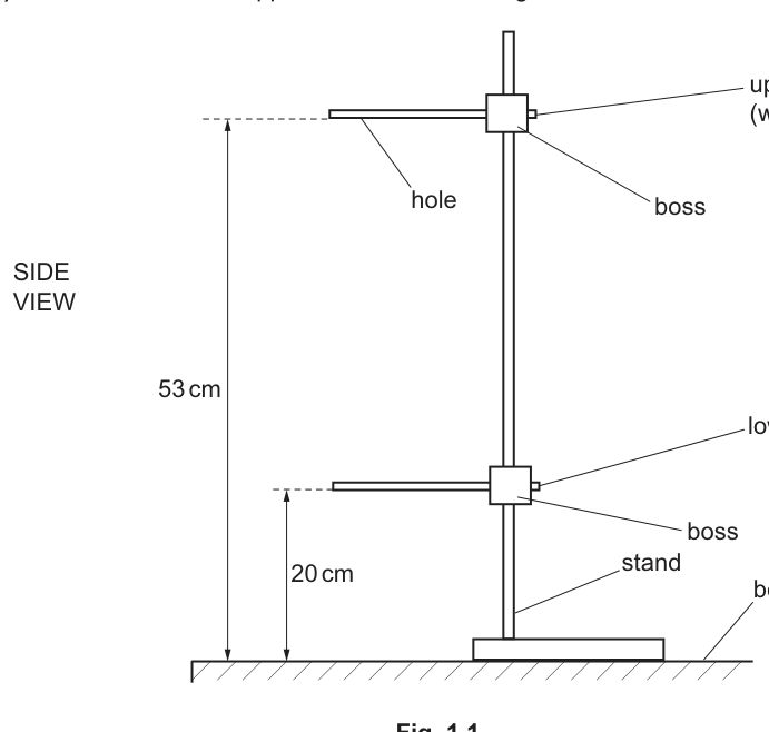
• Rotate the upper rod in the boss so that the hole is vertical.
• Thread the string of the pendulum up through the hole in the upper rod and pull it through until the pendulum bob is approximately $2\text{ cm}$ above the bench. Use the clip to fasten the string to the stand to prevent the string from slipping down through the hole, as shown in Fig. 1.2.

Fig. 1.2

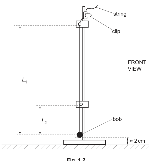
• Turn the lower rod horizontally so that the string is just touching the rod. Leave both rods in these positions for the whole experiment.
• The distance of the centre of the bob below the upper rod is $L_1$ . The distance of the centre of the bob below the lower rod is $L_2$ .

Measure and record $L_1$ and $L_2$ .

$L_1$ = ______
$L_2$ = ______

1M Similar

DifficultyEasy

Worked solution

Answer

Measure $L_1$ and $L_2$ vertically from the rods to the centre of the bob using a ruler (eye level to avoid parallax) and record to the nearest $1\ \text{mm}$ .

Example:

$L_1 = 0.500\ \text{m}$

$L_2 = 0.180\ \text{m}$

Final answer

Example: L1 = 0.500 m, L2 = 0.180 m

Detailed explanation

Background Concept

In practical work, length measurements must be made using a clearly defined reference point and recorded to the correct resolution.

Here, both $L_1$ and $L_2$ are vertical distances to the centre of the pendulum bob. A metre rule typically has $1\ \text{mm}$ divisions, so a careful reading can be recorded to the nearest $1\ \text{mm}$ (i.e. $0.001\ \text{m}$ ) or nearest $0.1\ \text{cm}$ , depending on unit choice.

Understanding the Question

You are given a pendulum set-up with two rods (upper and lower). You must measure:

$L_1$ : distance from the upper rod down to the centre of the bob,
$L_2$ : distance from the lower rod down to the centre of the bob,
and write the values in the answer spaces.

Approach

Decide the exact points between which the distance is defined (rod level to centre of bob).
Place the ruler so that it measures the vertical distance (not along the string).
Read the scale at eye level to avoid parallax.
Record with appropriate precision for the instrument.

Step-by-Step Reasoning

Identify the centre of the bob (this is the reference point for both $L_1$ and $L_2$ ).
Hold the ruler close to the bob and rods, aligned vertically.
For $L_1$ , read the ruler at the level of the upper rod and at the centre of the bob and take the difference (or measure directly if positioned conveniently).
Repeat for $L_2$ using the lower rod.
Record readings to the metre rule resolution (typically nearest $1\ \text{mm}$ ).

Key Takeaways

Always measure between the exact points defined in the question (centre of bob matters).
Keep the ruler vertical for a vertical distance.
Record to sensible precision consistent with the scale.

Common Mistakes

Measuring to the bottom of the bob instead of the centre.
Measuring along the string rather than vertically.
Parallax error from reading the ruler at an angle.
Overstating precision (e.g. writing many decimal places when using a metre rule).

Things to Be Careful About

Ensure the string is stationary when you read $L_1$ and $L_2$ .
Check which rod is used for $L_1$ vs $L_2$ .
Use consistent units (m or cm) for all subsequent calculations.

Techniques used

measure a vertical distance using a ruler with correct alignmentread a scale at eye level to reduce parallax erroridentify the centre of the bob and measure to that reference point

(ii)

• Push the bob so that the string moves a short distance away from the lower rod and then release it. The bob will oscillate.
• Take measurements to find the period $T$ of the oscillations.

$T$ = ______

2M Similar

DifficultyMedium-Easy

Worked solution

Working

Time $N$ oscillations ( $N \ge 10$ ) using a stopwatch and repeat.

Example:

$N = 10$

$t_1 = 10.2\ \text{s}$ , $t_2 = 10.1\ \text{s}$

Mean time for $10$ oscillations:

\bar{t} = \frac{10.2 + 10.1}{2} = 10.15\ \text{s}

T = \frac{\bar{t}}{N} = \frac{10.15}{10} = 1.02\ \text{s}

Answer

$T = 1.02\ \text{s}$ (example)

Final answer

Example: T = 1.02 s

Detailed explanation

Background Concept

The period $T$ is the time taken for one complete oscillation. With a stopwatch, reaction time introduces a large uncertainty if you time only one oscillation. Timing many oscillations reduces the fractional uncertainty because the reaction-time uncertainty is roughly the same size, but it becomes a smaller fraction of the total time.

If $t$ is the time for $N$ oscillations, then:

T = \frac{t}{N}

Repeating and averaging helps reduce random error.

Understanding the Question

You must "take measurements to find the period $T$ " for the pendulum oscillations. No single correct value exists because it depends on your measured length(s), so marks are typically for using a good method and recording a sensible value with unit.

Approach

Use a small amplitude (short push) so the motion is close to simple harmonic.
Choose a clear reference point (e.g. bob passing the equilibrium position in one direction).
Time $N \ge 10$ oscillations.
Repeat the timing and average.
Divide by $N$ to get $T$ .

Step-by-Step Reasoning

Displace the bob slightly and release without pushing.
Start the stopwatch as the bob passes a chosen point in a chosen direction.
Count oscillations: one oscillation means returning to the same position moving in the same direction.
Stop the stopwatch after $N$ oscillations at the same reference condition.
Repeat to get a second (or third) value of $t$ .
Calculate the mean time and then compute $T = \bar{t}/N$ .
Quote $T$ to a sensible precision (usually 2 or 3 s.f.) and include the unit $\text{s}$ .

Key Takeaways

Time many oscillations and divide.
Repeat and average.
Use a consistent definition of one oscillation.

Common Mistakes

Timing only one oscillation (large percentage uncertainty).
Counting half-oscillations (e.g. one swing) as a full oscillation.
Large amplitude, causing the period to change slightly.
Forgetting to divide by $N$ .

Things to Be Careful About

Keep the amplitude small and similar for all readings.
Avoid the bob hitting/touching the rod during timing if that would change the motion.
Start/stop timing at the same position each time.

Techniques used

time multiple oscillations and divide by the number of oscillationsrepeat timing measurements and calculate a mean valueuse a consistent reference point to define one oscillation

(b)

Move the string through the hole and refasten it to change $L_1$ . Measure and record $L_1$ , $L_2$ and $T$ .

Repeat until you have six sets of values of $L_1$ , $L_2$ and $T$ .

Record your results in a table. Include values of $(\sqrt{L_1} + \sqrt{L_2})$ to three significant figures in your table.

8M Similar

DifficultyMedium

Worked solution

Answer

Record six sets of $L_1$ , $L_2$ and $T$ , then calculate $(\sqrt{L_1}+\sqrt{L_2})$ and give it to three significant figures.

(Example table format and sample values)

$L_1 / \text{m}$	$L_2 / \text{m}$	$T / \text{s}$	$(\sqrt{L_1}+\sqrt{L_2}) / \text{m}^{1/2}$
0.550	0.250	1.26	1.24
0.520	0.220	1.21	1.19
0.490	0.190	1.16	1.14
0.460	0.160	1.10	1.08
0.430	0.130	1.04	1.02
0.400	0.100	0.97	0.948

Example of calculation (first row):

\sqrt{0.550} + \sqrt{0.250} = 0.742 + 0.500 = 1.242 \approx 1.24\ \text{m}^{1/2}

Final answer

Table of six sets with calculated (sqrt(L1)+sqrt(L2)) to 3 s.f. (see working)

Detailed explanation

Background Concept

A good results table in Paper 3 must:

contain all raw and derived data in one clear table,
have column headings with quantity and unit (e.g. $L_1/\text{m}$ ),
show consistent precision within a column,
include any calculated quantities to the precision requested.

Here you must compute $(\sqrt{L_1}+\sqrt{L_2})$ and quote it to three significant figures.

Understanding the Question

You must change $L_1$ (by moving the string through the hole) and each time measure and record:

$L_1$ , $L_2$ ,
the period $T$ .
You need six sets of values. Then you must add an extra column for $(\sqrt{L_1}+\sqrt{L_2})$ , rounded to 3 s.f.

Approach

Choose six different values of $L_1$ spread over a good range (not all very similar).
For each, measure $L_1$ and $L_2$ carefully.
Determine $T$ using a repeatable timing method (e.g. $N=10$ oscillations, repeated).
Fill a table with correct headings and units.
Calculate $(\sqrt{L_1}+\sqrt{L_2})$ for each row and round to 3 s.f.

Step-by-Step Reasoning

After setting a new $L_1$ , re-measure both $L_1$ and $L_2$ (because changing the string position changes both distances).
Measure the period $T$ consistently (same $N$ , similar amplitude), and preferably repeat to reduce random error.
When calculating $(\sqrt{L_1}+\sqrt{L_2})$ , ensure both lengths are in the same unit before square-rooting.
Round the final sum to three significant figures exactly as requested.
Check the trend: as lengths decrease, $(\sqrt{L_1}+\sqrt{L_2})$ should decrease, so $T$ should also tend to decrease if the suggested linear relationship is correct.

Key Takeaways

Tables need clear headings with units and consistent precision.
Derived quantities must be calculated correctly and rounded as instructed.
A good range of the independent variable improves the quality of the graph.

Common Mistakes

Missing units in headings (e.g. writing just $L_1$ instead of $L_1/\text{m}$ ).
Rounding intermediate square roots too early; better to keep extra digits then round the final sum.
Giving $(\sqrt{L_1}+\sqrt{L_2})$ to the wrong number of significant figures.
Using inconsistent decimal places for $T$ within the column.

Things to Be Careful About

Decide early whether you work in $\text{m}$ or $\text{cm}$ and keep it consistent throughout (especially for the graph and for later units of $a$ ).
Make sure each row corresponds to the same set of conditions (don’t mix $L_1$ from one run with $T$ from another).
Six distinct sets are required; do not repeat the same length values.

Techniques used

collect repeated sets of measurements while varying one variablerecord results in a table with headings and unitscalculate a derived quantity and quote it to the required significant figuresmaintain consistent decimal places within each column

(c)

(i)

Plot a graph of $T$ on the $y$ -axis against $(\sqrt{L_1} + \sqrt{L_2})$ on the $x$ -axis.

3M Similar

DifficultyMedium-Easy

Worked solution

Answer

Plot $T$ on the $y$ -axis against $(\sqrt{L_1}+\sqrt{L_2})$ on the $x$ -axis.

Label axes: $T/\text{s}$ and $(\sqrt{L_1}+\sqrt{L_2})/\text{m}^{1/2}$ .
Use a scale that uses at least half the grid on each axis.
Plot all six points with small, neat crosses.

Final answer

Graph of T (y) against (sqrt(L1)+sqrt(L2)) (x) with correct labels/scales and all points plotted

Detailed explanation

Background Concept

A graph is used to test whether two variables have a linear relationship. Marks are typically awarded for:

correct choice of axes (dependent variable on $y$ , independent on $x$ ),
correct axis labels including units,
sensible scales (not cramped, not awkward like 3, 6, 9 etc.),
accurate plotting.

Understanding the Question

You must produce a graph where:

$y$ -axis: $T$ ,
$x$ -axis: $(\sqrt{L_1}+\sqrt{L_2})$ .
This is already the linearised form of the suggested equation, so a straight line is expected if the model is valid.

Approach

Choose axes covering the full range of your data.
Mark a scale that makes it easy to plot (e.g. 0.05 or 0.1 per large square).
Plot each pair $\left((\sqrt{L_1}+\sqrt{L_2}),\ T\right)$ .

Step-by-Step Reasoning

Find the minimum and maximum of $(\sqrt{L_1}+\sqrt{L_2})$ and $T$ from your table.
Choose axis limits slightly beyond these extremes.
Label axes with the format quantity/unit, e.g. $T/\text{s}$ .
Plot each value carefully; use a sharp pencil and small crosses so the line can be drawn accurately later.

Key Takeaways

Axes must be labelled with both quantity and unit.
Scales should make full use of the graph paper.
Plotting accuracy directly affects gradient/intercept accuracy.

Common Mistakes

Swapping axes (plotting $T$ on $x$ ).
Missing units on axes.
Using a very small part of the grid, leading to large gradient uncertainty.
Plotting dots that are too large.

Things to Be Careful About

Ensure the derived quantity $(\sqrt{L_1}+\sqrt{L_2})$ is plotted to the stated precision (3 s.f.).
Don’t force the graph through the origin unless the data genuinely supports it.

Techniques used

label axes with quantity and unitchoose a sensible scale that uses most of the graph gridplot points accurately from a results table

(ii)

Draw the straight line of best fit.

1M Similar

(iii)

Determine the gradient and $y$ -intercept of this line.

gradient = ______
$y$ -intercept = ______

2M Similar

DifficultyMedium

Worked solution

Working

Using a large triangle on the best-fit line:

\text{gradient} = \frac{\Delta T}{\Delta(\sqrt{L_1}+\sqrt{L_2})}

Example values from the line:

\text{gradient} = 1.00\ \text{s m}^{-1/2}

Read $y$ -intercept at $(\sqrt{L_1}+\sqrt{L_2}) = 0$ :

\text{$y$-intercept} = 0.020\ \text{s}

Answer

gradient $= 1.00\ \text{s m}^{-1/2}$

$y$ -intercept $= 0.020\ \text{s}$ (example)

Final answer

Example: gradient = 1.00 s m^(-1/2), y-intercept = 0.020 s

Detailed explanation

Background Concept

For a straight-line graph, the gradient and intercept describe the relationship:

y = mx + c

Gradient $m$ is the change in $y$ per unit change in $x$ :

m = \frac{\Delta y}{\Delta x}

The $y$ -intercept $c$ is the value of $y$ where $x = 0$ .

In practical graphs, using a large triangle (spanning much of the line) reduces percentage uncertainty in the gradient.

Understanding the Question

You must find the gradient and $y$ -intercept of your best-fit line on the graph of $T$ (y-axis) against $(\sqrt{L_1}+\sqrt{L_2})$ (x-axis).

Approach

Choose two well-separated points on the best-fit line (not necessarily data points).
Read their coordinates accurately.
Calculate the gradient using $\Delta T/\Delta x$ .
Extend the best-fit line to $x=0$ (if necessary) and read the intercept.
Quote units:
- gradient unit $= \text{(unit of }T) / \text{(unit of }x)$ ,
- intercept unit is the same as $T$ .

Step-by-Step Reasoning

Suppose you select two points on the line: $(x_1, T_1)$ and $(x_2, T_2)$ .
Compute:

\Delta T = T_2 - T_1, \qquad \Delta x = x_2 - x_1

\text{gradient} = \frac{\Delta T}{\Delta x}

For the intercept, set $x=0$ and read where the line crosses the $T$ axis.
Check reasonableness: if the relationship is correct, points should lie close to the line and the gradient should be positive.

Key Takeaways

Always use a large triangle on the best-fit line.
Gradient is $\Delta y/\Delta x$ , not $y/x$ .
Intercept is read at $x=0$ .

Common Mistakes

Using two adjacent points (small triangle), giving a very uncertain gradient.
Using a plotted point that is not on the best-fit line.
Calculating $\Delta x/\Delta y$ by mistake.
Forgetting units or giving incorrect units for gradient.

Things to Be Careful About

Read coordinates to at least half a small square if possible.
Use consistent units: if $x$ is in $\text{m}^{1/2}$ , the gradient unit must include $\text{m}^{-1/2}$ .
Do not round gradient/intercept too aggressively; keep 2–3 significant figures consistent with graph precision.

Techniques used

use a large triangle on the best-fit line to calculate gradientcompute gradient as $\Delta y / \Delta x$read the y-intercept from the graph at $x = 0$

(d)

It is suggested that the quantities $T$ , $L_1$ and $L_2$ are related by the equation

T = a(\sqrt{L_1} + \sqrt{L_2}) + b

where $a$ and $b$ are constants.

Using your answers in (c)(iii), determine the values of $a$ and $b$ . Give appropriate units.

$a$ = ______
$b$ = ______

2M Similar

DifficultyMedium-Easy

Worked solution

Working

Given:

T = a(\sqrt{L_1}+\sqrt{L_2}) + b

Comparing with $y = mx + c$ for a graph of $T$ (y-axis) against $(\sqrt{L_1}+\sqrt{L_2})$ (x-axis):

a = \text{gradient}, \qquad b = y\text{-intercept}

Using (c)(iii) example values:

a = 1.00\ \text{s m}^{-1/2}

b = 0.020\ \text{s}

Answer

$a = 1.00\ \text{s m}^{-1/2}$

$b = 0.020\ \text{s}$

Final answer

Example: a = 1.00 s m^(-1/2), b = 0.020 s

Detailed explanation

Background Concept

When an equation has the form

y = mx + c

and you plot $y$ against $x$ , then:

the gradient of the straight line is $m$ ,
the $y$ -intercept is $c$ .

Units follow directly:

[m] = \frac{[y]}{[x]}, \qquad [c] = [y]

Understanding the Question

You are told:

T = a(\sqrt{L_1} + \sqrt{L_2}) + b

and you have already found the gradient and intercept from the graph of $T$ against $(\sqrt{L_1}+\sqrt{L_2})$ . You must use those to state $a$ and $b$ with appropriate units.

Approach

Identify $y \equiv T$ and $x \equiv (\sqrt{L_1}+\sqrt{L_2})$ .
Match the equation to $T = ax + b$ .
Therefore $a$ is the gradient and $b$ is the intercept.
Write the units based on your axis units.

Step-by-Step Reasoning

From your graph:
- gradient $= \Delta T/\Delta x$ .
- intercept is $T$ when $x=0$ .
Thus, numerically:

a = \text{gradient}

b = y\text{-intercept}

Units:
- If $T$ is in $\text{s}$ and $x$ is in $\text{m}^{1/2}$ , then

[a] = \frac{\text{s}}{\text{m}^{1/2}} = \text{s m}^{-1/2}

and

[b] = \text{s}

Key Takeaways

Linear plots allow constants to be read from gradient and intercept.
Always attach units to constants based on plotted quantities.

Common Mistakes

Swapping $a$ and $b$ .
Giving $a$ the same unit as $T$ (forgetting it is a gradient).
Quoting $b$ with the wrong unit (it must match $T$ ).

Things to Be Careful About

Your value of $a$ depends on the unit used for $L_1$ and $L_2$ . If you used $\text{cm}$ , your $a$ will be in $\text{s cm}^{-1/2}$ , not $\text{s m}^{-1/2}$ .
Keep consistent significant figures: the constant values should not look more precise than the graph allows.

Techniques used

compare an experimental straight-line graph with the form y = mx + cidentify constants as gradient and interceptassign units to constants from the units of the plotted variables

(e)

Theory suggests that $a$ is related to the acceleration of free fall $g$ by

g = \left( \frac{\pi}{a} \right)^2

Using your value for $a$ , calculate a value for $g$ . Give an appropriate unit.

$g$ = ______

1M Similar

DifficultyMedium-Easy

Worked solution

Working

Using

g = \left( \frac{\pi}{a} \right)^2

with $a = 1.00\ \text{s m}^{-1/2}$ :

g = \left( \frac{\pi}{1.00} \right)^2 = 9.87\ \text{m s}^{-2}

Answer

$g = 9.87\ \text{m s}^{-2}$

Final answer

g = 9.87 m s^-2

Detailed explanation

Background Concept

This part links an experimentally determined constant $a$ to the gravitational field strength $g$ using:

g = \left( \frac{\pi}{a} \right)^2

Because $\pi$ is dimensionless, the unit of $g$ depends on the unit of $a$ . If $a$ has units $\text{s m}^{-1/2}$ , then:

\left[\frac{1}{a}\right] = \text{m}^{1/2}\text{s}^{-1} \Rightarrow \left[\left(\frac{1}{a}\right)^2\right] = \text{m s}^{-2}

which matches the expected unit for $g$ .

Understanding the Question

You must take your value of $a$ (from the graph) and calculate $g$ using the given formula. You must also provide an appropriate unit.

Approach

Substitute your experimental value of $a$ into the formula.
Calculate $\pi/a$ .
Square the result to get $g$ .
Quote $g$ in $\text{m s}^{-2}$ if your $a$ was based on metres (or convert if needed).

Step-by-Step Reasoning

Start with:

g = \left( \frac{\pi}{a} \right)^2

Substitute your measured $a$ .
Evaluate the bracket first, then square.
Unit check:
- If $a$ is $\text{s m}^{-1/2}$ then $g$ will come out in $\text{m s}^{-2}$ .
- If instead you used $L$ in cm so $a$ is $\text{s cm}^{-1/2}$ , then $g$ would come out in $\text{cm s}^{-2}$ and must be divided by $100$ to express in $\text{m s}^{-2}$ .

Key Takeaways

Substitute carefully and do powers in the correct order.
Units depend on the units used earlier in the experiment.

Common Mistakes

Forgetting to square the bracket.
Using $g = (a/\pi)^2$ (inverting the expression incorrectly).
Giving $g$ in the wrong unit because $L$ was measured in cm.

Things to Be Careful About

Significant figures: $g$ should not be quoted more precisely than $a$ .
If your $a$ is close to $1.00\ \text{s m}^{-1/2}$ , you should obtain $g$ close to $9.8\ \text{m s}^{-2}$ . A very different value suggests a unit or calculation error.

Techniques used

substitute an experimentally determined constant into a given formularearrange and evaluate an expression involving powerscheck dimensional consistency and quote the correct unit

Q2MediumManipulation, Measurement and ObservationAnalysis, Conclusions and EvaluationPresentation of Data and Observations

In this experiment, you will investigate the motion of steel balls falling through water in a tube.

(a)

(i)

You have been provided with a wide tube attached to a wooden strip.

Measure and record the internal diameter $D$ of the wide tube.

$D$ = ______

2M Similar

DifficultyMedium-Easy

Worked solution

Measure internal diameter using vernier calipers (internal jaws); take several readings around the tube and average.

Example:

D = 28.6\ \text{mm}

Final answer

Example: D = 28.6 mm

Detailed explanation

Background Concept

For practical measurements, marks are usually awarded for (i) choosing a suitable instrument, (ii) using it correctly, and (iii) recording to the instrument’s resolution with a unit.

For an internal diameter, vernier calipers are appropriate because they have internal jaws designed to touch the inside walls. The reading should be recorded consistently (typically to the nearest $0.1\ \text{mm}$ for a vernier caliper, depending on the scale provided).

Understanding the Question

You are given a wide tube and asked to measure and record its internal diameter $D$ . Since the tube may not be perfectly circular, taking more than one reading at different orientations/positions improves reliability.

Approach

Use the internal jaws of vernier calipers.
Take readings at a few positions (e.g. rotate the calipers by $90^\circ$ and/or measure at different heights).
Calculate a mean value.
Record $D$ with unit and to a consistent precision.

Step-by-Step Reasoning

Open the internal jaws slightly, insert them into the tube, and expand until they just touch the inner walls.
Ensure the calipers are across the diameter (not at a slant).
Read the main scale and vernier scale (or digital reading).
Repeat at least twice more.
Average the readings and record as $D$ .

An example of an appropriately recorded value is:

D = 28.6\ \text{mm}

Key Takeaways

Internal diameters should be measured with the internal jaws of vernier calipers.
Repeats can account for ovality and reduce random error.
Always include a unit and sensible precision.

Common Mistakes

Measuring the external diameter instead of the internal diameter.
Recording too many decimal places (beyond the caliper resolution) or too few.
Not including a unit.
Measuring at an angle so the jaws do not span the true diameter.

Things to Be Careful About

Gentle contact: do not compress the tube or force the jaws.
If the tube is slightly oval, quote a mean of several orientations.
Keep the same unit (mm or cm) consistently for later calculations (especially when squaring).

Techniques used

use vernier calipers internal jaws to measure an internal diametertake repeat readings at different positions and calculate a meanrecord a measurement to an appropriate resolution with unit

(ii)

• Assemble the apparatus as shown in Fig. 2.1.

Fig. 2.1

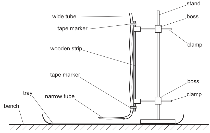
You have been provided with four steel balls of two different diameters.

• Measure and record the diameter $d$ of one of the larger balls.

$d$ = ______

• Fill the syringe with water from the beaker.
• Push the nozzle of the syringe securely into the narrow tube. Slowly push the syringe plunger until the wide tube is filled to the top with water. Leave the syringe attached to the narrow tube.
• Drop one of the larger balls into the wide tube and watch it fall down past the two tape markers.
• Use the magnet to retrieve the ball from the tube.

1M Similar

(b)

(i)

• Drop one of the larger balls into the wide tube.
• Take measurements to determine the time $t$ for the ball to fall from the upper tape marker to the lower tape marker.

$t$ = ______

2M Similar

DifficultyMedium-Easy

Worked solution

Time the fall between the two tape markers with a stopwatch; repeat and average.

Example (3 trials): $3.52\ \text{s}$ , $3.47\ \text{s}$ , $3.51\ \text{s}$

Mean:

t = \frac{3.52 + 3.47 + 3.51}{3} = 3.50\ \text{s}

Final answer

Example: t = 3.50 s

Detailed explanation

Background Concept

Timing a moving object with a stopwatch is limited by human reaction time and by how clearly you can identify the start and stop events. Repeating the measurement and taking an average reduces random error.

In this experiment, $t$ is the time for the ball to travel from the upper tape marker to the lower tape marker. To keep results consistent, you must always start timing at the same event (e.g. when the bottom of the ball reaches the upper marker) and stop at the corresponding event at the lower marker.

Understanding the Question

You drop a larger ball into the water-filled wide tube and must determine the time $t$ for it to move between the two tape markers. The answer is a measured value of $t$ (with unit) obtained by an appropriate set of readings.

Approach

Drop the ball from the top and allow it to pass the upper marker.
Start timing as the ball passes the upper marker; stop as it passes the lower marker.
Repeat at least 3 times and calculate the mean $t$ .

Step-by-Step Reasoning

Ensure the tube is vertical and the water level is at the top as instructed.
Release the ball without pushing it sideways.
Observe the ball at the marker; start the stopwatch at the chosen reference point on the ball.
Stop the stopwatch at the same reference point when the ball reaches the lower marker.
Repeat.

Example set of readings:

$t_1 = 3.52\ \text{s}$
$t_2 = 3.47\ \text{s}$
$t_3 = 3.51\ \text{s}$

Mean:

t = \frac{t_1+t_2+t_3}{3} = 3.50\ \text{s}

Key Takeaways

Use repeated timings and a mean.
Use a consistent definition of when timing starts/stops.
Record with appropriate precision (typically to $0.01\ \text{s}$ if a digital stopwatch is used).

Common Mistakes

Only taking one timing.
Starting timing when the ball is released rather than when it reaches the upper marker.
Using different reference points on the ball for start and stop.

Things to Be Careful About

The ball may accelerate initially; the markers are used to define a fixed measured interval regardless.
Make sure your eye is level with the marker to reduce parallax.
If the ball wobbles or hits the wall, discard that run and repeat.

Techniques used

time an event using a stopwatch between two reference markersrepeat measurements and calculate a mean valueensure consistent start/stop criteria for timing

(ii)

Estimate the percentage uncertainty in your value of $t$ . Show your working.

percentage uncertainty = ______ $\%$

1M Similar

DifficultyMedium-Easy

Worked solution

Take stopwatch uncertainty (reaction time at start and stop) as $\pm 0.2\ \text{s}$ .

\%\ \text{uncertainty in } t = \frac{0.2}{3.50} \times 100 = 5.7\%\,(\approx 6\%)

Final answer

5.7% (≈ 6%)

Detailed explanation

Background Concept

Percentage uncertainty is found from

\%\ \text{uncertainty} = \frac{\text{absolute uncertainty}}{\text{measured value}} \times 100.

For stopwatch timings, a common estimate for absolute uncertainty is based on human reaction time. Because you react at both the start and stop, the combined uncertainty is often taken as about $\pm 0.2\ \text{s}$ (or another sensible value consistent with your timing method).

Alternatively, if repeats are taken, an absolute uncertainty can be estimated from the spread (e.g. half the range of repeated values).

Understanding the Question

You must estimate the percentage uncertainty in your measured time $t$ (from part (b)(i)) and show working. This is about uncertainty in the timing measurement, not about $D$ or $d$ .

Approach

Choose a reasonable absolute uncertainty for $t$ (reaction time or half-range).
Divide by your measured $t$ and multiply by $100$ .

Step-by-Step Reasoning

Using the example mean time $t = 3.50\ \text{s}$ :

Take reaction-time uncertainty as $\pm 0.2\ \text{s}$ (start + stop).
Then

\%\ \text{uncertainty} = \frac{0.2}{3.50} \times 100 = 5.7\%.

So you may quote about $6\%$ .

Key Takeaways

Percentage uncertainty comes from absolute uncertainty divided by the measured value.
State clearly where your absolute uncertainty comes from.

Common Mistakes

Using $\pm 0.1\ \text{s}$ for a single reaction, but forgetting there are two reactions (start and stop).
Calculating $\frac{t}{\Delta t}$ instead of $\frac{\Delta t}{t}$ .
Giving an uncertainty to an over-precise number of decimal places.

Things to Be Careful About

If you used repeats and the spread is larger than reaction time suggests, use the spread-based estimate.
Make sure the uncertainty value you choose is realistic for your method and stated clearly.

Techniques used

estimate an absolute uncertainty from reaction time or spread of repeatscalculate percentage uncertainty using absolute uncertainty divided by measured valuepresent uncertainty to a sensible number of significant figures

(c)

• Measure and record the diameter $d$ of one of the smaller balls.

$d$ = ______

• Using one of the smaller balls, repeat (b)(i).

$t$ = ______

3M Similar

DifficultyMedium-Easy

Worked solution

Measure diameter of a smaller ball.

Example:

d = 20.00\ \text{mm}

Repeat the timing between tape markers with the smaller ball (repeat and average).

Example (3 trials): $1.66\ \text{s}$ , $1.63\ \text{s}$ , $1.66\ \text{s}$

Mean:

t = \frac{1.66 + 1.63 + 1.66}{3} = 1.65\ \text{s}

Final answer

Example: d = 20.00 mm, t = 1.65 s

Detailed explanation

Background Concept

To compare two balls, you must keep the method the same so that any change in measured time is due to the change in ball diameter rather than changes in procedure. Diameter measurement should be to the instrument resolution, and timing should be repeated and averaged.

Understanding the Question

You must (1) measure and record the diameter $d$ of a smaller ball, and (2) using a smaller ball, repeat the timing procedure from (b)(i) to obtain $t$ between the same two tape markers.

Approach

Measure $d$ with micrometer/callipers, ideally with repeats and rotation.
Drop the smaller ball and measure time between the same two markers.
Repeat timings and calculate mean $t$ .

Step-by-Step Reasoning

Measure the smaller ball diameter:
- Use the micrometer ratchet for consistent pressure.
- Rotate ball and repeat; take the mean.
- Example:
$d = 20.00\ \text{mm}$
Time the fall between the two markers:
- Use the same start/stop definition as for the larger ball.
- Repeat 3 times and average.
- Example readings: $1.66\ \text{s}$ , $1.63\ \text{s}$ , $1.66\ \text{s}$ .
- Mean:
$t = 1.65\ \text{s}$

Key Takeaways

Keep conditions constant (same tube, same marker separation, same water conditions) when comparing runs.
Repeat measurements to reduce random uncertainty.

Common Mistakes

Measuring $d$ with inconsistent precision compared with the larger ball measurement.
Using a different start/stop criterion than before.
Not repeating the timing.

Things to Be Careful About

Ensure the ball does not stick to the tube wall; if it does, repeat the run.
If water temperature changes noticeably, viscosity changes and times may drift.

Techniques used

measure a sphere diameter with a suitable instrument and appropriate precisiontime motion between two reference markers with repeats and averagingkeep the procedure consistent between two sets of readings

(d)

It is suggested that the relationship between $t$ , $D$ and $d$ is

\frac{1}{t} = k(D^2 - d^2)

where $k$ is a constant.

(i)

Using your data, calculate two values of $k$ .

first value of $k$ = ______
second value of $k$ = ______

1M Similar

DifficultyMedium

Worked solution

From

\frac{1}{t} = k(D^2-d^2)

k = \frac{1/t}{D^2-d^2}.

Using $D=0.0286\ \text{m}$ .

Larger ball: $d=0.0250\ \text{m}$ , $t=3.50\ \text{s}$

D^2-d^2 = (0.0286)^2-(0.0250)^2 = 1.93\times 10^{-4}\ \text{m}^2

k = \frac{1/3.50}{1.93\times 10^{-4}} = 1.48\times 10^{3}\ \text{s}^{-1}\ \text{m}^{-2}

Smaller ball: $d=0.0200\ \text{m}$ , $t=1.65\ \text{s}$

D^2-d^2 = (0.0286)^2-(0.0200)^2 = 4.18\times 10^{-4}\ \text{m}^2

k = \frac{1/1.65}{4.18\times 10^{-4}} = 1.45\times 10^{3}\ \text{s}^{-1}\ \text{m}^{-2}

Final answer

First k = 1.48×10^3 s^-1 m^-2; second k = 1.45×10^3 s^-1 m^-2

Detailed explanation

Background Concept

If a relationship is suggested in the form

\frac{1}{t} = k(D^2-d^2),

then for any set of measured values of $t$ , $D$ and $d$ , you can calculate the constant $k$ by rearranging:

k = \frac{1/t}{D^2-d^2}.

Because $D$ and $d$ are squared, unit consistency is essential: if you use mm for one value and m for another, $D^2-d^2$ becomes meaningless. A safe approach is to convert all lengths to metres.

Understanding the Question

You have two datasets (one for a larger ball and one for a smaller ball). You must use each dataset to calculate a value of $k$ and then you will later compare them.

Approach

Rearrange to get $k$ as the subject.
Convert $D$ and $d$ to consistent units.
Compute $D^2-d^2$ for each ball.
Compute $1/t$ for each case.
Divide to obtain $k$ twice.

Step-by-Step Reasoning

Rearrange:

k = \frac{1/t}{D^2-d^2}.

Using example measured values:

$D = 28.6\ \text{mm} = 0.0286\ \text{m}$ .

Larger ball

$d = 25.00\ \text{mm} = 0.0250\ \text{m}$
$t = 3.50\ \text{s}$ so $1/t = 0.2857\ \text{s}^{-1}$
Compute the squared difference:

D^2-d^2 = (0.0286)^2-(0.0250)^2 = 1.93\times 10^{-4}\ \text{m}^2

Then

k = \frac{0.2857}{1.93\times 10^{-4}} \approx 1.48\times 10^{3}\ \text{s}^{-1}\ \text{m}^{-2}.

Smaller ball

$d = 20.00\ \text{mm} = 0.0200\ \text{m}$
$t = 1.65\ \text{s}$ so $1/t = 0.6061\ \text{s}^{-1}$
Compute:

D^2-d^2 = (0.0286)^2-(0.0200)^2 = 4.18\times 10^{-4}\ \text{m}^2

Then

k = \frac{0.6061}{4.18\times 10^{-4}} \approx 1.45\times 10^{3}\ \text{s}^{-1}\ \text{m}^{-2}.

The closeness of these two values is what you use in part (e).

Key Takeaways

Rearrangement skills: isolate $k$ .
Consistent units matter especially when squaring.
Two values of a constant let you test whether a relationship is supported.

Common Mistakes

Using mm in the calculation without being consistent, causing $D^2-d^2$ to be in mixed units.
Squaring only one of the diameters (e.g. using $D^2-d$ ).
Forgetting that $1/t$ has units $\text{s}^{-1}$ .

Things to Be Careful About

If $D$ and $d$ are close, $D^2-d^2$ can be small, so rounding too early can change $k$ noticeably.
Keep extra digits during intermediate steps, then round the final $k$ to justified significant figures.

Techniques used

rearrange an equation to solve for a constantsubstitute measured values consistently in SI unitscalculate and report two independent values for comparison

(ii)

Justify the number of significant figures that you have given for your values of $k$ .

1M Similar

DifficultyMedium-Easy

Worked solution

The values of $k$ depend on measured $D$ , $d$ and $t$ .

$D$ and $d$ are recorded to about 3 s.f. (e.g. $28.6\ \text{mm}$ ) and $t$ to about 3 s.f. (e.g. $3.50\ \text{s}$ ), so $k$ should be given to 3 s.f.

Final answer

k to 3 significant figures

Detailed explanation

Background Concept

Significant figures communicate the precision of a value. A calculated quantity should not be quoted to a precision higher than the least precise measurement used to calculate it.

Here,

k = \frac{1/t}{D^2-d^2},

so $k$ depends on $D$ , $d$ and $t$ . Because $D$ and $d$ are squared and subtracted, excessive rounding can strongly affect $D^2-d^2$ , so it is important not to over-round intermediate steps.

Understanding the Question

You must explain (justify) the number of significant figures used for your two values of $k$ . This is not asking for a recalculation; it is asking for an argument based on measurement precision.

Approach

Identify the precision of the raw measurements ( $D$ , $d$ , $t$ ).
Choose the significant figures of $k$ to be consistent with the least precise of those.
Mention that intermediate rounding should be avoided.

Step-by-Step Reasoning

Suppose $D$ was recorded as $28.6\ \text{mm}$ (3 s.f.) using vernier calipers.
Suppose $d$ was recorded as $25.00\ \text{mm}$ (4 s.f.) using a micrometer.
Suppose $t$ was recorded as $3.50\ \text{s}$ (3 s.f.).

The limiting precision is then about 3 s.f. (from $D$ and $t$ ). Therefore quoting $k$ to 3 s.f. is justified (e.g. $1.48\times 10^3$ rather than $1.48237\times 10^3$ ).

Key Takeaways

Do not claim more precision in $k$ than exists in the measurements.
Keep extra digits during working; round only at the end.

Common Mistakes

Quoting $k$ to 1 or 2 s.f. when the measurements justify 3 s.f. (unnecessarily crude).
Quoting $k$ to 4–5 s.f. because the calculator displays them.

Things to Be Careful About

If your timing uncertainty is dominated by reaction time, the true precision of $t$ may be worse than the stopwatch resolution; that can reduce the justified significant figures for $k$ .
Subtraction in $D^2-d^2$ can increase percentage uncertainty if $D$ and $d$ are close, so avoid premature rounding.

Techniques used

identify the least precisely measured quantitiesmatch the significant figures of a derived quantity to the input dataavoid over-rounding intermediate calculations

(e)

It is suggested that the percentage uncertainty in the values of $k$ is $10\%$ .

Using this uncertainty, explain whether your results support the relationship in (d).

1M Similar

DifficultyMedium

Worked solution

Using $k_1 = 1.48\times 10^3$ and $k_2 = 1.45\times 10^3$ :

\%\ \text{difference} = \frac{|k_1-k_2|}{\frac{k_1+k_2}{2}}\times 100 = \frac{30}{1465}\times 100 \approx 2.0\%.

Since $2.0\% < 10\%$ , the two values agree within the uncertainty, so the results support the relationship.

Final answer

Yes, supports (values agree within 10%).

Detailed explanation

Background Concept

When a relationship predicts that a constant $k$ should be the same for different trials, you test it by calculating $k$ from each trial and checking whether the values agree within experimental uncertainty.

A simple way is to calculate a percentage difference between the two values and compare it with the stated percentage uncertainty.

Understanding the Question

You are told to assume the percentage uncertainty in the values of $k$ is $10\%$ . You must decide whether your two calculated values of $k$ are consistent with each other (and hence whether the suggested relationship is supported).

Approach

Compute the percentage difference between your two $k$ values.
If the difference is less than (or comparable to) $10\%$ , the results support the relationship.

Step-by-Step Reasoning

Using example values:

$k_1 = 1.48\times 10^3\ \text{s}^{-1}\ \text{m}^{-2}$
$k_2 = 1.45\times 10^3\ \text{s}^{-1}\ \text{m}^{-2}$

Difference:

|k_1-k_2| = 30.

Mean:

\frac{k_1+k_2}{2} = \frac{1480+1450}{2} = 1465.

Percentage difference:

\frac{30}{1465}\times 100 \approx 2.0\%.

Because $2.0\%$ is well below $10\%$ , the two values of $k$ agree within the uncertainty. Therefore the experimental results support the proposed relationship.

Key Takeaways

A relationship is supported if repeated/varied trials give a consistent constant within uncertainty.
Use a quantitative comparison, not just “they look similar”.

Common Mistakes

Comparing absolute differences without scaling (e.g. saying “difference is 30” without context).
Using $\frac{|k_1-k_2|}{k_1}$ instead of comparing with the mean (either can be acceptable, but must be applied sensibly).
Concluding “does not support” even when values differ by less than the stated uncertainty.

Things to Be Careful About

The stated $10\%$ is a percentage uncertainty in $k$ , so your comparison should also be in percentage terms.
If your two values differ by around $10\%$ , it is safer to say “consistent within uncertainty” rather than “proves the relationship”.

Techniques used

compare two experimental values using a percentage differencejudge agreement using a stated percentage uncertaintystate a clear conclusion linked to the comparison

(f)

(i)

Describe four sources of uncertainty or limitations of the procedure for this experiment.

For any uncertainties in measurement that you describe, you should state the quantity being measured and a reason for the uncertainty.

4M Similar

DifficultyMedium-Easy

Worked solution

Timing $t$ : uncertainty due to human reaction time starting/stopping stopwatch as ball passes a marker.
Timing $t$ : difficulty judging the exact instant the ball aligns with the tape marker (parallax / finite marker thickness).
Motion of ball: ball may not fall centrally; it can touch the tube wall, changing the resistive forces and hence $t$ .
Conditions of water: temperature may change during the experiment so viscosity changes, affecting the fall time.

(Any four suitable, clearly distinct limitations.)

Final answer

See working (four limitations stated).

Detailed explanation

Background Concept

In evaluation questions, marks are awarded for specific sources of uncertainty/limitations that are clearly linked to a measured quantity and a physical reason. Vague statements like “human error” usually gain no credit.

Uncertainties can be:

Random (e.g. reaction time variations) which cause scatter and are reduced by repeats.
Systematic (e.g. consistent delay in starting/stopping, mis-measured diameters) which shift results.

Understanding the Question

You must describe four sources of uncertainty or limitations in this falling-ball-in-water procedure. For measurement uncertainties, you must state the quantity (e.g. $t$ , $D$ , $d$ ) and explain why it is uncertain.

Approach

Pick four different issues, preferably covering both measurement and physical-process limitations:

timing,
marker alignment/visibility,
ball motion in tube,
water properties,
diameter measurements.

Step-by-Step Reasoning

Examples of creditworthy points:

Timing $t$ (reaction time): starting and stopping a stopwatch as the ball passes a marker involves reaction time, giving an absolute uncertainty (often about $\pm 0.2\ \text{s}$ combined).
Timing $t$ (deciding the instant): the ball and marker have finite size; it is hard to judge when the same point on the ball is exactly level with the tape. Viewing angle causes parallax.
Ball path / wall contact: if the ball is off-centre or hits the wall, the resistive/drag forces differ and the ball may slow, changing $t$ in an uncontrolled way.
Water viscosity / temperature: viscosity depends on temperature; if temperature changes during the experiment, $t$ changes even for the same ball.

Other acceptable limitations (any could replace one of the above):

Air bubbles sticking to ball or tube wall change effective drag/buoyancy.
Diameter measurements $D$ and $d$ : limited by instrument resolution and possible zero error; for $D$ the tube may be slightly oval.
Tube not perfectly vertical: introduces sideways component, encouraging wall contact and changing motion.

Key Takeaways

Always name the quantity affected and the reason.
Provide distinct points, not four versions of “timing is hard”.

Common Mistakes

Writing “human error” without specifying what was measured.
Repeating the same limitation in different words (e.g. four timing points).
Listing an “improvement” instead of a limitation.

Things to Be Careful About

If you mention measurement uncertainty, tie it to the instrument (resolution, zero error, parallax) or the method (reaction time, alignment).
Make sure each of your four points is genuinely different.

Techniques used

identify measurement uncertainties and link each to a quantityexplain the physical reason behind each uncertainty/limitationstate distinct limitations without repeating the same idea

(ii)

Describe four improvements that could be made to this experiment. You may suggest the use of other apparatus or different procedures.

4M Similar

DifficultyMedium-Easy

Worked solution

Use light gates (or video analysis) at the two marker positions to measure $t$ automatically and remove reaction-time uncertainty.
Increase the separation of the markers so $t$ is larger, reducing fractional timing uncertainty.
Repeat each timing several times and take a mean; reject runs where the ball touches the wall.
Control water temperature (e.g. water bath / allow to reach room temperature before measurements) to keep viscosity constant.

(Any four suitable improvements.)

Final answer

See working (four improvements stated).

Detailed explanation

Background Concept

Improvements should be specific actions that reduce the uncertainties/limitations identified. Strong answers pair an improvement with the problem it fixes (e.g. “use light gates” because “stopwatch reaction time is large”).

Understanding the Question

You must describe four improvements to the experiment. You may suggest different apparatus or changed procedures. The goal is to reduce uncertainty in $t$ , $D$ , $d$ , and to make the motion more consistent.

Approach

Choose improvements that target major error sources:

timing method,
marker definition,
ball path control,
stability of fluid conditions,
better measurement instruments and repeats.

Step-by-Step Reasoning

Examples of well-justified improvements:

Replace stopwatch timing: Use two light gates connected to an electronic timer/data logger at the marker positions (or record video and use frame counting). This removes reaction time and gives a clear start/stop event.
Reduce fractional timing uncertainty: Increase the distance between markers so the measured time is longer; the same absolute timing uncertainty then corresponds to a smaller percentage uncertainty.
Improve reliability: Perform more repeats for each ball and take an average; discard anomalous runs (e.g. ball visibly contacts wall) to reduce random scatter.
Control fluid properties: Keep water temperature constant (insulate tube or use a water bath) and remove bubbles before runs. This stabilises viscosity and drag.

Other acceptable improvements:

Use a guide/release mechanism to drop the ball centrally.
Ensure tube is vertical using a plumb line/spirit level.
Use micrometer for ball diameter and apply zero-error correction; measure $D$ at several orientations and average.

Key Takeaways

Improvements must be practical and must reduce a named uncertainty.
Automatic timing methods are a common high-impact improvement.

Common Mistakes

Suggesting an improvement that does not address any real limitation (e.g. “use a better ruler” when the dominant uncertainty is timing).
Giving vague ideas (“be more careful”).
Repeating the same improvement four times in different words.

Things to Be Careful About

Ensure each improvement is distinct (timing, alignment, temperature, repeats, etc.).
Keep suggestions realistic for a school/college laboratory setting.

Techniques used

propose procedural changes that directly address stated limitationssuggest alternative apparatus to reduce measurement uncertaintyincrease reliability by repeating and improving measurement definition