In this experiment, you will investigate the motion of steel balls falling through water in a tube. (i) You have been provided with a wide tube attached to a wooden strip. Measure and record the internal diameter $D$ of the wide tube. $D$ = \_\_\_\_\_\_ (ii) • Assemble the apparatus as shown in Fig. 2.1. • You have been provided with four steel balls of two different diameters. • Measure and record the diameter $d$ of one of the larger balls. $d$ = \_\_\_\_\_\_ • Fill the…

(a)(i) D ≈ 28.0 mm · (a)(ii) d ≈ 10.0 mm · (b)(i) t ≈ 5.03 s · (b)(ii) 8.0 % · (c) d ≈ 8.0 mm, t ≈ 4.70 s · (d)(i) k1 ≈ 2.91×10^2 s^-1 m^-2, k2 ≈ 2.96×10^2 s^-1 m^-2 · (d)(ii) k quoted to 3 s.f. (limited by D, d and t measurements) · (e) Yes, k values agree within 10% so relationship is supported. · (f)(i) Four limitations: stopwatch reaction; judging crossing of marker; uncertainty in ball diameter; ball path/wall contact affects drag. · (f)(ii) Four improvements:…

Physics 9702/34 — May/June 2025

Cambridge AS Level · Advanced Practical Skills · worked solutions for every part, with the mark scheme

questions

marks

120

minutes

Topics Manipulation, Measurement and Observation · Presentation of Data and Observations · Analysis, Conclusions and Evaluation

Q1MediumManipulation, Measurement and ObservationPresentation of Data and ObservationsAnalysis, Conclusions and Evaluation

In this experiment, you will investigate the properties of a pendulum.

(a)

(i)

• Assemble the apparatus as shown in Fig. 1.1.

Fig. 1.1

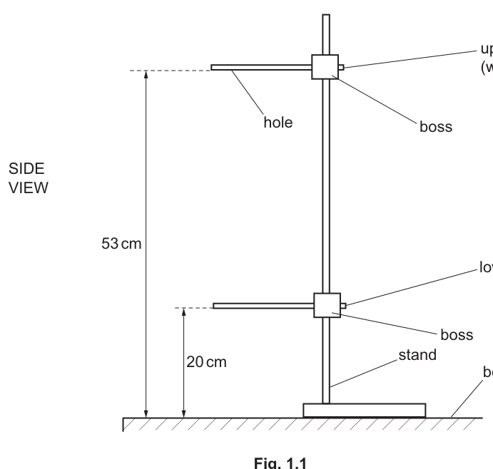
• Rotate the upper rod in the boss so that the hole is vertical.

• Thread the string of the pendulum up through the hole in the upper rod and pull it through until the pendulum bob is approximately $2\text{ cm}$ above the bench. Use the clip to fasten the string to the stand to prevent the string from slipping down through the hole, as shown in Fig. 1.2.

Fig. 1.2

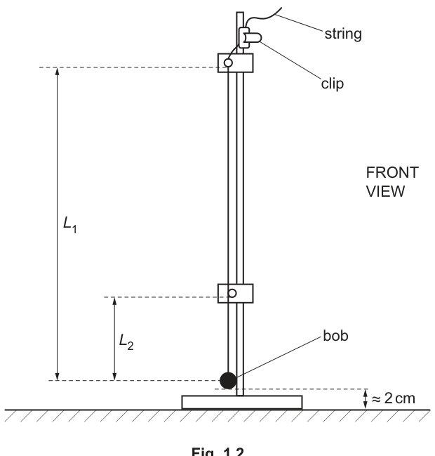
• Turn the lower rod horizontally so that the string is just touching the rod. Leave both rods in these positions for the whole experiment.

• The distance of the centre of the bob below the upper rod is $L_1$ . The distance of the centre of the bob below the lower rod is $L_2$ .

Measure and record $L_1$ and $L_2$ .

$L_1$ = ______
$L_2$ = ______

1M Similar

DifficultyEasy

Worked solution

Answer

Measure from the upper rod (at the hole) to the centre of the bob to get $L_1$ , and from the lower rod to the centre of the bob to get $L_2$ .

Example (to nearest $1\ \text{mm}$ ):

$L_1 = 0.510\ \text{m}$

$L_2 = 0.180\ \text{m}$

Final answer

Student-dependent (e.g. L1 = 0.510 m, L2 = 0.180 m)

Detailed explanation

Background Concept

In a practical experiment, a length measurement must be defined by:

clear reference points (exactly where the measurement starts and ends), and
a stated precision (set by the measuring instrument, e.g. a metre rule).

Here, both lengths are vertical distances to the centre of the bob:

$L_1$ : upper rod (\to) centre of bob
$L_2$ : lower rod (\to) centre of bob

To gain marks in Paper 3, the key is usually correct identification of what to measure and recording the value with sensible precision (typically metre rule to nearest $1\ \text{mm}$ or $0.1\ \text{cm}$ ).

Understanding the Question

You are instructed to set up the apparatus and then measure and record $L_1$ and $L_2$ as defined in the text/diagram:

$L_1$ is the distance of the bob’s centre below the upper rod.
$L_2$ is the distance of the bob’s centre below the lower rod.

These values will be used later to calculate (\sqrt{L_1}+\sqrt{L_2}), so you need measurements that are as accurate and repeatable as possible.

Approach

Ensure the apparatus is in the required fixed geometry (rods left in place for the whole experiment).
Use a metre rule alongside the string/bob.
Measure each distance as a vertical distance to the centre of the bob.
Record each to appropriate precision and with units.

Step-by-Step Reasoning

Place the metre rule close to the string so you can read vertical distances without parallax.
For $L_1$ , identify the level of the upper rod at the hole (the point where the string passes through) and measure down to the bob’s centre.
For $L_2$ , identify the level of the lower rod and measure down to the bob’s centre.
Read the scale at eye level to reduce parallax error.
Record values to the nearest division of the rule (commonly $1\ \text{mm}$ ).

A typical set of readings for the geometry shown might be around $L_1 \approx 0.5\ \text{m}$ and $L_2 \approx 0.2\ \text{m}$ , but your exact values depend on where you clamp the string.

Key Takeaways

Always measure between the defined points (rod level to bob centre).
Record to an appropriate precision with units.
Avoid parallax by reading the scale at eye level.

Common Mistakes

Measuring to the bottom of the bob instead of its centre.
Measuring along the string at an angle rather than vertically.
Recording lengths without units, or with inconsistent precision.

Things to Be Careful About

Keep rods fixed as instructed; moving them changes the geometry and makes later comparisons invalid.
Use the same precision for all $L_1$ readings and for all $L_2$ readings (consistency in a data set matters).

Techniques used

identify the correct reference points for a length measurementmeasure a vertical distance with a metre rule to appropriate precisionrecord readings with consistent precision and units

(ii)

• Push the bob so that the string moves a short distance away from the lower rod and then release it. The bob will oscillate.

• Take measurements to find the period $T$ of the oscillations.

$T$ = ______

2M Similar

DifficultyMedium-Easy

Worked solution

Working

Time $N$ oscillations (e.g. $N=10$ ) and divide by $N$ .

Example:

T = \frac{t}{N} = \frac{11.4\ \text{s}}{10} = 1.14\ \text{s}

Answer

$T = 1.14\ \text{s}$ (example)

Final answer

Student-dependent (e.g. T = 1.14 s)

Detailed explanation

Background Concept

The period $T$ is the time taken for one complete oscillation. Using a stopwatch to time one oscillation gives a large percentage uncertainty because human reaction time (often around $0.2\ \text{s}$ ) is a big fraction of $T$ .

A standard improvement is to time multiple oscillations:

T = \frac{t}{N}

where:

$t$ is the total time for $N$ oscillations,
$N$ is a reasonably large integer (often $10$ or more).

This reduces the percentage uncertainty because the same reaction-time error is spread over a larger total time.

Understanding the Question

You are asked to “take measurements to find the period $T$ ”. This means you must describe/perform a timing method and record a value of $T$ in seconds.

The bob is oscillating as a pendulum, and you must choose a consistent point in the swing (e.g. passing a fixed reference point) to start/stop timing.

Approach

Choose a reference point (fiducial mark), e.g. the equilibrium position.
Start timing as the bob passes the reference point in a chosen direction.
Count $N$ complete oscillations.
Stop timing when the bob next passes the reference point after $N$ oscillations in the same direction.
Compute $T=t/N$ .
Repeat and average.

Step-by-Step Reasoning

Displace the bob by a small angle and release it (small amplitude helps keep the motion closer to simple harmonic motion and makes timing more consistent).
Decide on $N$ (e.g. $10$ or $20$ ).
Use the same direction of crossing (e.g. left-to-right) for both start and stop to ensure you measure whole oscillations.
Suppose you measure $t = 11.4\ \text{s}$ for $N=10$ oscillations.
Then: $T = \frac{11.4\ \text{s}}{10} = 1.14\ \text{s}$
Repeat the measurement (e.g. twice more) and take the mean $T$ ; this reduces random scatter.

Key Takeaways

Time many oscillations: $T=t/N$ .
Use a fixed reference point and the same crossing direction.
Repeat and average to improve reliability.

Common Mistakes

Timing only one oscillation (large percentage uncertainty).
Not counting complete oscillations correctly (off by 1).
Starting and stopping at different points in the motion (inconsistent reference).

Things to Be Careful About

Keep the amplitude small and similar for each run.
Ensure the string does not slip through the hole (clip must hold it firmly), otherwise $L_1$ and $L_2$ change during timing.

Techniques used

time multiple oscillations and divide to find the perioduse a fiducial marker to define a consistent timing pointrepeat timings and average to reduce random uncertainty

(b)

Move the string through the hole and refasten it to change $L_1$ . Measure and record $L_1$ , $L_2$ and $T$ .

Repeat until you have six sets of values of $L_1$ , $L_2$ and $T$ .

Record your results in a table. Include values of $(\sqrt{L_1} + \sqrt{L_2})$ to three significant figures in your table.

8M Similar

DifficultyMedium

Worked solution

Answer

Record six sets of $L_1$ , $L_2$ and $T$ and calculate $(\sqrt{L_1}+\sqrt{L_2})$ to three significant figures.

Example table (headings include units):

$L_1 / \text{m}$	$L_2 / \text{m}$	$T / \text{s}$	$(\sqrt{L_1}+\sqrt{L_2}) / \text{m}^{1/2}$
0.430	0.100	0.97	0.972
0.450	0.120	1.02	1.02
0.470	0.140	1.06	1.06
0.490	0.160	1.10	1.10
0.510	0.180	1.14	1.14
0.530	0.200	1.18	1.18

Final answer

Student-dependent (table of six sets including (sqrt(L1)+sqrt(L2)) to 3 s.f.)

Detailed explanation

Background Concept

In Paper 3, marks for tables are usually awarded for:

a single clear table containing all readings,
correct headings: quantity symbol and unit (e.g. $L_1/\text{m}$ ),
consistent precision for raw readings (all $L_1$ to the same decimal place, etc.),
correct calculation of any derived quantity, here $(\sqrt{L_1}+\sqrt{L_2})$ to three significant figures.

A good experiment also uses a suitable range of the independent variable (here you change $L_1$ by moving the string) so the graph later is meaningful.

Understanding the Question

You must:

Change $L_1$ (by moving the string through the hole and refastening it).
Measure and record $L_1$ , $L_2$ , and the period $T$ .
Repeat until you have six sets.
Add a calculated column for $(\sqrt{L_1}+\sqrt{L_2})$ rounded to 3 s.f.

Approach

Choose six different positions of the bob (hence six values of $L_1$ ), spread out over as wide a range as is practical.
For each setting:
- measure $L_1$ and $L_2$ with the same instrument and same precision,
- measure $T$ by timing many oscillations and dividing by the number,
- compute $(\sqrt{L_1}+\sqrt{L_2})$ and round to 3 s.f.
Put everything in a single table with correct headings.

Step-by-Step Reasoning

After each adjustment of the string, let the bob come to rest and re-check the string is still just touching the lower rod (as instructed).
Measure $L_1$ and $L_2$ (vertical distances to the bob centre) and record them.
Measure the period $T$ using e.g. $N=10$ oscillations: $T = \frac{t}{N}$
Calculate the derived quantity: $x = \sqrt{L_1}+\sqrt{L_2}$ and round $x$ to three significant figures.

For example, if $L_1=0.510\ \text{m}$ and $L_2=0.180\ \text{m}$ :

\sqrt{L_1} = \sqrt{0.510} = 0.714\ \text{m}^{1/2},\qquad \sqrt{L_2} = \sqrt{0.180} = 0.424\ \text{m}^{1/2}

\sqrt{L_1}+\sqrt{L_2} = 1.138\ \text{m}^{1/2} \approx 1.14\ \text{m}^{1/2}\ (3\ \text{s.f.})

Key Takeaways

Six sets of results with a good spread improves the quality of a best-fit line.
Table marks depend heavily on presentation: headings, units, and consistent precision.
Derived values must be rounded exactly as instructed (3 s.f.).

Common Mistakes

Missing units in the table headings.
Mixing precision (e.g. some $L_1$ to $0.1\ \text{cm}$ and others to $0.01\ \text{cm}$ ).
Calculating $(\sqrt{L_1}+\sqrt{L_2})$ but not rounding to three significant figures.
Using different units for different rows (e.g. some lengths in cm, some in m).

Things to Be Careful About

If you use cm for $L_1$ and $L_2$ , then $(\sqrt{L_1}+\sqrt{L_2})$ has units $\text{cm}^{1/2}$ . That is allowed as long as you are consistent, but later calculations for $g$ are simplest in SI units (m and s).
When taking square roots, keep enough digits in the calculator and only round the final summed value to 3 s.f.

Techniques used

vary the independent variable over a suitable range and take multiple sets of readingstabulate raw and derived quantities with correct headings and unitscalculate a derived column and round to the required significant figuresmaintain consistent decimal places within each raw-data column

(c)

(i)

Plot a graph of $T$ on the $y$ -axis against $(\sqrt{L_1} + \sqrt{L_2})$ on the $x$ -axis.

3M Similar

DifficultyMedium-Easy

Worked solution

Answer

Plot $T$ on the $y$ -axis and $(\sqrt{L_1}+\sqrt{L_2})$ on the $x$ -axis.

Label axes with units (e.g. $T/\text{s}$ and $(\sqrt{L_1}+\sqrt{L_2})/\text{m}^{1/2}$ ), use a sensible scale occupying at least half the grid, and plot all six points accurately.

Final answer

Graph plotted: T vs (sqrt(L1)+sqrt(L2)) with correct labels/scales/points

Detailed explanation

Background Concept

Graph marks in Paper 3 usually come from:

correct choice of axes (correct variables),
correct axis labels including units,
sensible scales (linear, not awkward, using much of the grid),
accurate plotting (small, neat points or crosses).

Understanding the Question

You must plot a graph with:

$y$ -axis: $T$
$x$ -axis: $(\sqrt{L_1}+\sqrt{L_2})$

This is designed so that if the suggested relationship is correct, you should later obtain a straight line.

Approach

Compute $(\sqrt{L_1}+\sqrt{L_2})$ for each row of your table.
Draw axes and choose scales that cover the full range of your data.
Label each axis with both the quantity and the unit.
Plot all points carefully.

Step-by-Step Reasoning

Find the minimum and maximum of $(\sqrt{L_1}+\sqrt{L_2})$ and of $T$ .
Choose scales so the plotted points spread over a large area of the grid (this reduces fractional reading error when drawing a best-fit line and finding gradient).
Label axes in the accepted form, e.g.
- $T / \text{s}$
- $(\sqrt{L_1}+\sqrt{L_2}) / \text{m}^{1/2}$ (or $\text{cm}^{1/2}$ if you used cm consistently)
Plot each point as a small cross (recommended) and ensure points are not blobs.

Key Takeaways

Correct variables on axes and correct units are essential.
Good scale choice improves the precision of gradient/intercept.

Common Mistakes

Swapping axes (putting $T$ on $x$ ).
Missing units in axis labels.
Using a scale that wastes space (points squeezed into a corner).
Plotting from unrounded intermediate values inconsistently with the table.

Things to Be Careful About

Do not force the graph to start at zero unless it helps; choose a scale that best fits your data range.
Keep consistent: if your table uses $(\sqrt{L_1}+\sqrt{L_2})$ to 3 s.f., plot those same values.

Techniques used

choose suitable linear scales that use most of the graph gridlabel axes with quantity and unitplot points accurately from a table of values

(ii)

Draw the straight line of best fit.

1M Similar

(iii)

Determine the gradient and $y$ -intercept of this line.

gradient = ______
$y$ -intercept = ______

2M Similar

DifficultyMedium

Worked solution

Working

Using two well-separated points on the best-fit line (example):

(x_1,y_1)=(0.98\ \text{m}^{1/2},\ 0.98\ \text{s}),\quad (x_2,y_2)=(1.18\ \text{m}^{1/2},\ 1.18\ \text{s})

\text{gradient} = \frac{\Delta y}{\Delta x} = \frac{1.18-0.98}{1.18-0.98} = 1.00\ \text{s m}^{-1/2}

Extrapolating the line to $x=0$ gives (example) $y$ -intercept $= 0.00\ \text{s}$ .

Answer

gradient $= 1.00\ \text{s m}^{-1/2}$

$y$ -intercept $= 0.00\ \text{s}$

Final answer

Student-dependent (gradient and y-intercept from best-fit line, e.g. 1.00 s m^{-1/2} and 0.00 s)

Detailed explanation

Background Concept

For a straight-line graph of the form

y = mx + c

the gradient is $m=\Delta y/\Delta x$ (rate of change of $y$ with $x$ ),
the y-intercept is $c$ (the value of $y$ when $x=0$ ).

On experimental graphs, you should find $m$ using a large triangle on the best-fit line to reduce percentage uncertainty.

Understanding the Question

You have plotted $T$ against $(\sqrt{L_1}+\sqrt{L_2})$ and drawn a best-fit straight line. Now you must extract:

gradient of the line,
y-intercept of the line.

These will later be used to find constants $a$ and $b$ in a suggested equation.

Approach

Pick two points far apart on the best-fit line (not necessarily measured data points).
Read their coordinates $(x_1,y_1)$ and $(x_2,y_2)$ .
Compute $m = (y_2-y_1)/(x_2-x_1)$ .
Extend the line to cut the $y$ -axis (where $x=0$ ) and read off $c$ .

Step-by-Step Reasoning

diagram-1

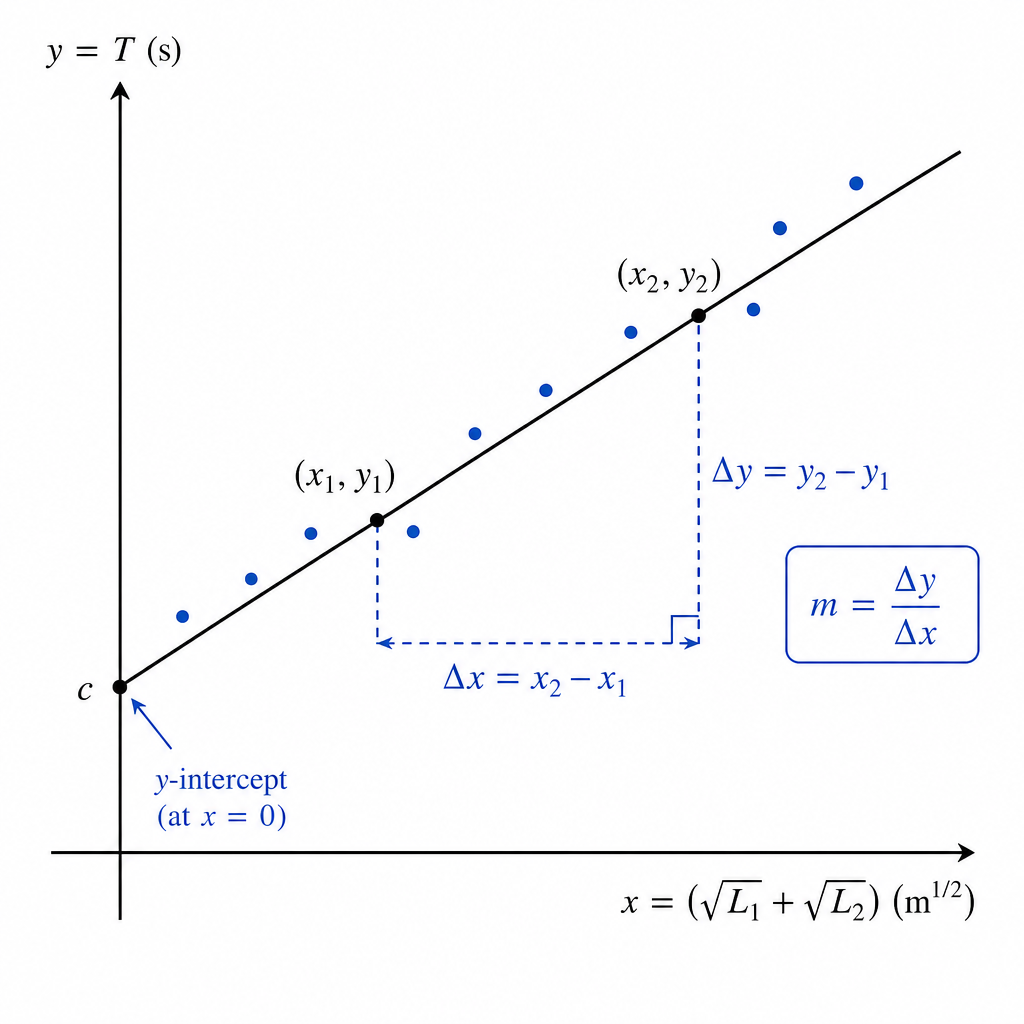
Choose two points with a large horizontal separation (large $\Delta x$ ) to reduce the effect of reading error.
Suppose the coordinates read from the line are: $(x_1,y_1)=(0.98,0.98),\quad (x_2,y_2)=(1.18,1.18)$ with $x$ in $\text{m}^{1/2}$ and $y$ in s.
Then: $m = \frac{\Delta y}{\Delta x} = \frac{1.18-0.98}{1.18-0.98} = 1.00$
Units: since $m = \Delta T/\Delta(\sqrt{L_1}+\sqrt{L_2})$ , $[m] = \frac{\text{s}}{\text{m}^{1/2}} = \text{s m}^{-1/2}$
For the intercept, extend the best-fit line to $x=0$ and read $T$ where it crosses the $y$ -axis. That value has units of seconds.

Your numerical values will depend on your plotted data; the method is what is assessed.

Key Takeaways

Use a large triangle on the best-fit line: $m=\Delta y/\Delta x$ .
Intercept is the $y$ value when $x=0$ .
Always include units for gradient and intercept.

Common Mistakes

Using two adjacent points (small triangle) leading to a very uncertain gradient.
Using data points rather than points on the best-fit line (can bias the gradient).
Calculating $\Delta x/\Delta y$ instead of $\Delta y/\Delta x$ .
Forgetting units, especially for the gradient.

Things to Be Careful About

Read coordinates accurately (use grid lines, not guesswork).
Ensure the line is extended carefully to the $y$ -axis for the intercept.
If you used cm in the table, your gradient unit becomes $\text{s cm}^{-1/2}$ ; keep the same unit consistently into part (d).

Techniques used

use a large triangle on the best-fit line to calculate the gradientread coordinates from the graph with correct unitsdetermine the y-intercept by extrapolation to x = 0

(d)

It is suggested that the quantities $T$ , $L_1$ and $L_2$ are related by the equation

T = a(\sqrt{L_1} + \sqrt{L_2}) + b

where $a$ and $b$ are constants.

Using your answers in (c)(iii), determine the values of $a$ and $b$ . Give appropriate units.

$a$ = ______
$b$ = ______

2M Similar

DifficultyMedium-Easy

Worked solution

Working

Given

T = a(\sqrt{L_1}+\sqrt{L_2}) + b

Comparing with $y = mx + c$ for the graph of $T$ (y-axis) against $(\sqrt{L_1}+\sqrt{L_2})$ (x-axis):

a = \text{gradient},\quad b = \text{y-intercept}

Using (c)(iii) (example):

a = 1.00\ \text{s m}^{-1/2}

b = 0.00\ \text{s}

Answer

$a = 1.00\ \text{s m}^{-1/2}$

$b = 0.00\ \text{s}$

Final answer

a = gradient, b = y-intercept (units consistent with axes)

Detailed explanation

Background Concept

If you plot $y$ against $x$ and the relationship is linear:

y = mx + c

then:

gradient $m$ is the constant multiplying $x$ ,
intercept $c$ is the value of $y$ when $x=0$ .

Units:

$m$ has units of $y/x$ ,
$c$ has the same units as $y$ .

Understanding the Question

You are given a suggested relationship:

T = a(\sqrt{L_1}+\sqrt{L_2}) + b

You have already made a graph of $T$ against $(\sqrt{L_1}+\sqrt{L_2})$ and found its gradient and intercept. You must use those graph values to determine $a$ and $b$ (with units).

Approach

Identify $y\equiv T$ and $x\equiv (\sqrt{L_1}+\sqrt{L_2})$ .
Compare directly with $y=mx+c$ .
Set $a=m$ and $b=c$ .
Write the units from your axis units.

Step-by-Step Reasoning

From the graph definition:

vertical axis: $T$ (seconds)
horizontal axis: $(\sqrt{L_1}+\sqrt{L_2})$ (e.g. $\text{m}^{1/2}$ )

So the straight-line equation is:

T = (\text{gradient})\,(\sqrt{L_1}+\sqrt{L_2}) + (\text{y-intercept})

Comparing with the suggested equation gives:

a = \text{gradient},\qquad b = \text{y-intercept}

Units:

[a] = \frac{\text{s}}{\text{m}^{1/2}} = \text{s m}^{-1/2},\qquad [b] = \text{s}

(or $\text{s cm}^{-1/2}$ if lengths were in cm).

Key Takeaways

Matching to $y=mx+c$ is the key link between graphs and equations.
Gradient gives the multiplier of $x$ ; intercept gives the constant term.
Units come from axis units.

Common Mistakes

Swapping $a$ and $b$ .
Quoting $a$ with unit s (forgetting it is a gradient).
Using units inconsistent with the graph (e.g. mixing cm and m partway through).

Things to Be Careful About

If you used cm for $L_1$ and $L_2$ , then $a$ will be in $\text{s cm}^{-1/2}$ . Converting to SI before calculating $g$ in part (e) avoids unit confusion.

Techniques used

match a linear equation to y = mx + cidentify constants as gradient and interceptassign units to constants from the plotted variables

(e)

Theory suggests that $a$ is related to the acceleration of free fall $g$ by

g = \left( \frac{\pi}{a} \right)^2

Using your value for $a$ , calculate a value for $g$ . Give an appropriate unit.

$g$ = ______

1M Similar

DifficultyMedium-Easy

Worked solution

Working

Using

g = \left( \frac{\pi}{a} \right)^2

With $a = 1.00\ \text{s m}^{-1/2}$ (example):

g = \left( \frac{\pi}{1.00} \right)^2 = 9.87\ \text{m s}^{-2}

Answer

$g = 9.87\ \text{m s}^{-2}$ (example)

Final answer

Student-dependent (e.g. g = 9.87 m s^{-2})

Detailed explanation

Background Concept

This step uses a provided theoretical link between the experimentally determined constant $a$ and gravitational field strength $g$ :

g = \left( \frac{\pi}{a} \right)^2

Dimensional check (if lengths are in metres):

$a$ has units $\text{s m}^{-1/2}$ ,
$\pi/a$ has units $\text{m}^{1/2}\text{s}^{-1}$ ,
squaring gives $\text{m s}^{-2}$ , the correct unit for $g$ .

Understanding the Question

You must take your value of $a$ from part (d) (found from the graph gradient) and substitute into the formula to calculate $g$ , then give an appropriate unit.

Approach

Use your experimental value of $a$ .
Substitute into $g=(\pi/a)^2$ .
Ensure units are consistent (ideally $a$ in $\text{s m}^{-1/2}$ ).
Round sensibly (usually 3 s.f. unless your data justify fewer).

Step-by-Step Reasoning

From part (d), take your gradient value $a$ .
Substitute: $g = \left( \frac{\pi}{a} \right)^2$
Example using $a=1.00\ \text{s m}^{-1/2}$ : $g = \left( \frac{3.142}{1.00} \right)^2 = 9.87$
Since the unit comes out as $\text{m s}^{-2}$ (when $a$ is in $\text{s m}^{-1/2}$ ), write: $g = 9.87\ \text{m s}^{-2}$

If your $a$ was found using $\text{cm}^{1/2}$ on the x-axis, you must convert so that $g$ is expressed in SI units. The safest method is to convert $L_1$ and $L_2$ into metres before graphing so $a$ is already in $\text{s m}^{-1/2}$ .

Key Takeaways

Substitute the gradient-derived constant into the given relationship.
Unit consistency matters; aim for SI so that $g$ is in $\text{m s}^{-2}$ .

Common Mistakes

Using $g=(\pi a)^2$ instead of $g=(\pi/a)^2$ .
Forgetting to square the bracket.
Getting a non-SI unit for $g$ by using $a$ in $\text{s cm}^{-1/2}$ and not converting.

Things to Be Careful About

Significant figures: $g$ cannot be more precise than $a$ (which comes from a graph and is usually 2–3 s.f.).
Keep calculator precision until the final step, then round once.

Techniques used

substitute a measured constant into a given formulahandle units consistently to obtain an SI unit for accelerationround the final result to appropriate significant figures

Q2MediumManipulation, Measurement and ObservationAnalysis, Conclusions and EvaluationPresentation of Data and Observations

In this experiment, you will investigate the motion of steel balls falling through water in a tube.

(a)

(i)

You have been provided with a wide tube attached to a wooden strip.

Measure and record the internal diameter $D$ of the wide tube.

$D$ = ______

2M Similar

DifficultyMedium-Easy

Worked solution

Answer

Example reading (to nearest $0.1\ \text{mm}$ ):

$D = 28.0\ \text{mm}$

Final answer

D ≈ 28.0 mm

Detailed explanation

Background Concept

Internal diameter is measured using the inside jaws of a vernier caliper. A good measurement is one that (i) uses the correct part of the instrument, (ii) is taken square across the diameter (not at a slant), and (iii) is recorded to the instrument resolution.

Understanding the Question

You are given a wide tube. You must measure and record its internal diameter $D$ (not the outside diameter). The mark is usually for a sensible value and correct recording (unit + appropriate decimal places).

Approach

Use vernier calipers and the internal jaws.
Measure the inside diameter across the tube.
Repeat at a couple of positions/rotations (tubes are not perfectly circular) and take a mean.
Record $D$ with a unit and to the caliper resolution.

Step-by-Step Reasoning

Open the internal jaws slightly larger than the tube opening.
Place the internal jaws inside the tube so they touch opposite internal walls.
Ensure the jaws are across a true diameter (jaws aligned through the centre).
Read the vernier scale and record $D$ (typically to $0.1\ \text{mm}$ for many school verniers).
Repeat after rotating the calipers by about $90^\circ$ and/or at a different height on the tube, then average.

A correctly recorded example would be $D = 28.0\ \text{mm}$ (unit included, consistent with $0.1\ \text{mm}$ resolution).

Key Takeaways

Use the internal jaws for internal diameter.
Repeat measurements to reduce random error and account for non-circular tubes.
Record with unit and correct precision.

Common Mistakes

Measuring the external diameter instead of internal.
Forgetting the unit.
Writing too many decimal places (implies unrealistic precision).
Taking only one reading when the tube may not be perfectly circular.

Things to Be Careful About

Avoid parallax when reading the vernier scale.
Make sure the calipers are not tilted; a tilted measurement underestimates the diameter.
Do not squeeze the tube (if flexible) as it can change the diameter slightly.

Techniques used

use a vernier caliper to measure an internal diametertake readings at several orientations and averagerecord a measurement to an appropriate instrument resolution

(ii)

• Assemble the apparatus as shown in Fig. 2.1.

Fig. 2.1

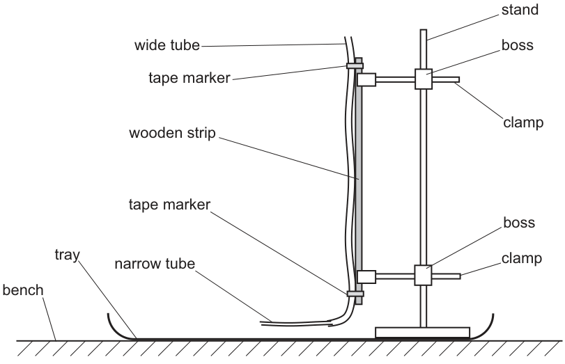
• You have been provided with four steel balls of two different diameters.

• Measure and record the diameter $d$ of one of the larger balls.

$d$ = ______

• Fill the syringe with water from the beaker.

• Push the nozzle of the syringe securely into the narrow tube. Slowly push the syringe plunger until the wide tube is filled to the top with water. Leave the syringe attached to the narrow tube.

• Drop one of the larger balls into the wide tube and watch it fall down past the two tape markers.

• Use the magnet to retrieve the ball from the tube.

1M Similar

DifficultyEasy

Worked solution

Answer

Example reading:

$d = 10.0\ \text{mm}$

Final answer

d ≈ 10.0 mm

Detailed explanation

Background Concept

The diameter of a steel ball is best measured with a micrometer screw gauge (high resolution, e.g. $0.01\ \text{mm}$ ) or vernier calipers (often $0.1\ \text{mm}$ ). Because the ball is small and rigid, you can take repeat readings in different orientations to check for slight non-sphericity.

Understanding the Question

You must (1) assemble the apparatus as in Fig. 2.1 and (2) measure the diameter $d$ of a larger steel ball and record it. The written answer space is for the value of $d$ .

Approach

Set up the tube vertically with two tape markers.
Fill the wide tube fully with water using the syringe (reduces bubbles and ensures consistent conditions).
Measure the ball diameter using micrometer/calipers; repeat and average; record with unit.

Step-by-Step Reasoning

diagram-a-ii

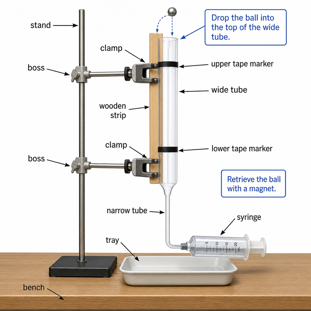
Assemble the stand, boss and clamp so that the wooden strip and wide tube are vertical and secure.
Ensure the two tape markers are fixed on the wide tube.
Fill syringe, attach to the narrow tube, and slowly push water until the wide tube is full to the top (helps minimise trapped air bubbles).
Measure the larger ball diameter $d$ $d$ :
- Place ball between micrometer anvils and tighten gently using the ratchet (prevents over-compression/extra force).
- Take at least two readings with the ball rotated and average.
Record $d$ with correct unit and precision (e.g. $10.0\ \text{mm}$ ).

Key Takeaways

Correct set-up (vertical tube, secure clamps) improves repeatability.
Measure $d$ carefully and record with appropriate precision.

Common Mistakes

Not filling the tube completely, leaving bubbles that affect motion.
Measuring the ball with excessive force (can give a smaller reading on some instruments).
Omitting the unit.

Things to Be Careful About

Keep the syringe attached as instructed so water level/conditions remain stable.
Ensure the tube is vertical; a tilted tube encourages the ball to touch the wall more often.
If using a micrometer, use the ratchet for consistent contact force.

Techniques used

set up apparatus as shown in a diagrammeasure a small diameter using an appropriate instrumentrecord a measurement with correct unit and precision

(b)

(i)

• Drop one of the larger balls into the wide tube.

• Take measurements to determine the time $t$ for the ball to fall from the upper tape marker to the lower tape marker.

$t$ = ______

2M Similar

DifficultyMedium-Easy

Worked solution

Working

Example repeat timings between the two tape markers:

$5.02\ \text{s},\ 5.08\ \text{s},\ 5.00\ \text{s}$

Mean time:

\bar{t} = \frac{5.02 + 5.08 + 5.00}{3} = 5.03\ \text{s}

Answer

$t = 5.03\ \text{s}$

Final answer

t ≈ 5.03 s

Detailed explanation

Background Concept

Timing a moving object with a handheld stopwatch is limited mainly by human reaction time (starting and stopping late/early). Random timing error can be reduced by repeating measurements and taking a mean. A larger timing interval also reduces the percentage uncertainty.

Understanding the Question

You must determine the time $t$ for a larger ball to fall from the upper tape marker to the lower tape marker. You are expected to take measurements (typically repeated) and then record a single value of $t$ .

Approach

Decide exactly when you will start and stop the timer (e.g. when the front of the ball crosses each marker).
Repeat the timing several times under the same conditions.
Calculate the mean $t$ and record it with suitable precision.

Step-by-Step Reasoning

diagram-b-i

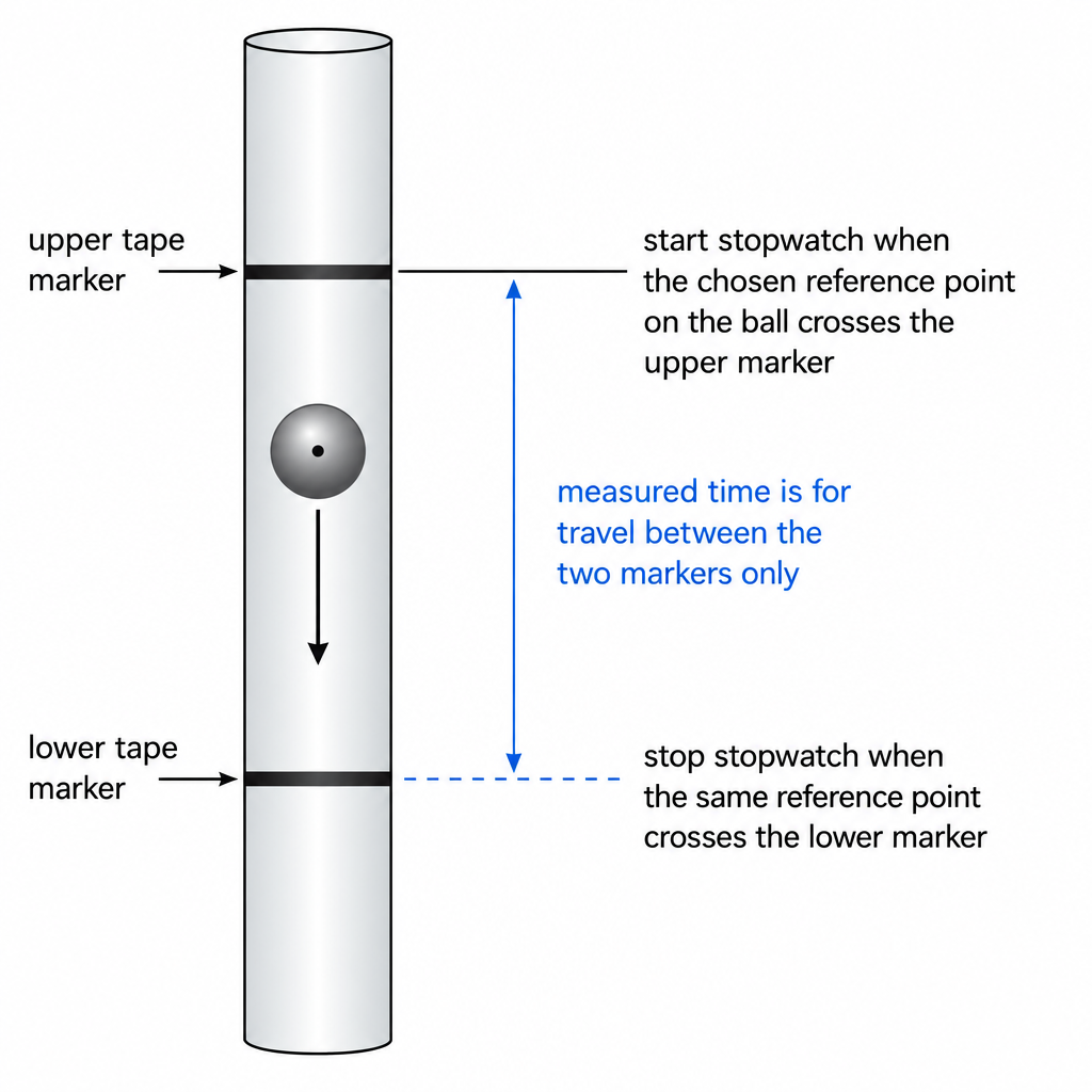
Drop the ball into the water at the top of the tube without pushing it (a push changes the motion).
Start the stopwatch as the ball crosses the upper tape marker (use a consistent reference point: top of ball or centre).
Stop the stopwatch as the ball crosses the lower tape marker.
Record the time.
Repeat at least two more times and compute the mean:

\bar{t} = \frac{t_1 + t_2 + t_3}{3}

This reduces random scatter from reaction time.

Key Takeaways

Use a consistent start/stop criterion at the markers.
Repeat and average to improve reliability.
Record time to match the stopwatch resolution (but remember reaction time dominates).

Common Mistakes

Timing from release at the top rather than between the tape markers.
Using different criteria each time (e.g. sometimes timing centre of ball, sometimes leading edge).
Only taking one timing.

Things to Be Careful About

Make sure the ball does not stick to the wall or pause at the start.
Keep the water level the same (tube full as instructed).
If the ball accelerates significantly between markers, repeated timings will vary more; ensure the markers are placed in a region where motion is steady (if possible).

Techniques used

time a moving object between two fixed markersrepeat measurements and calculate a mean valuerecord time measurements to appropriate resolution

(ii)

Estimate the percentage uncertainty in your value of $t$ . Show your working.

percentage uncertainty = ______ %

1M Similar

DifficultyMedium-Easy

Worked solution

Working

Take reaction time uncertainty as $\pm 0.2\ \text{s}$ for start and $\pm 0.2\ \text{s}$ for stop:

\Delta t \approx 0.4\ \text{s}

\%\ \text{uncertainty} = \frac{\Delta t}{t} \times 100 = \frac{0.4}{5.03} \times 100 = 8.0\%

Answer

percentage uncertainty $= 8.0\%$

Final answer

8.0 %

Detailed explanation

Background Concept

For a time measured with a handheld stopwatch, the limiting uncertainty is usually reaction time, not the stopwatch resolution. If you start late/early by about $\pm 0.2\ \text{s}$ and stop late/early by about $\pm 0.2\ \text{s}$ , then the total absolute uncertainty in the measured interval is roughly the sum:

\Delta t \approx 0.2 + 0.2 = 0.4\ \text{s}

Percentage uncertainty is:

\frac{\Delta t}{t} \times 100\%

Understanding the Question

You must estimate the percentage uncertainty in your measured time $t$ for the larger ball between the tape markers, and show working.

Approach

Choose a reasonable absolute uncertainty in $t$ (reaction time start + stop).
Divide by the measured $t$ and multiply by $100$ .
Quote the result to a sensible number of significant figures.

Step-by-Step Reasoning

Assume reaction time uncertainty $\pm 0.2\ \text{s}$ at each button press.
Combine for the measured interval:

\Delta t \approx 0.4\ \text{s}

Use your measured mean time (example $t = 5.03\ \text{s}$ ):

\%\ \text{uncertainty} = \frac{0.4}{5.03} \times 100 = 8.0\%

If your own measured $t$ differs, your percentage uncertainty will change accordingly.

Key Takeaways

Stopwatch timing uncertainty is often dominated by reaction time.
Total timing uncertainty for a single interval includes both the start and stop uncertainties.

Common Mistakes

Using only $\pm 0.2\ \text{s}$ total (forgetting there are two button presses).
Using the stopwatch resolution (e.g. $\pm 0.01\ \text{s}$ ) unrealistically.
Forgetting to multiply by $100$ .

Things to Be Careful About

If you time many oscillations/events and divide, the reaction-time contribution is reduced; here you time a single fall, so reaction time is significant.
Quote the percentage uncertainty sensibly (usually 1–2 s.f.).

Techniques used

estimate an absolute uncertainty from reaction timecalculate a percentage uncertaintyquote uncertainty to an appropriate number of significant figures

(c)

• Measure and record the diameter $d$ of one of the smaller balls.

$d$ = ______

• Using one of the smaller balls, repeat (b)(i).

$t$ = ______

3M Similar

DifficultyMedium-Easy

Worked solution

Working

Example reading for smaller ball diameter:

$d = 8.0\ \text{mm}$

Example repeat timings between markers (smaller ball):

$4.68\ \text{s},\ 4.74\ \text{s},\ 4.68\ \text{s}$

\bar{t} = \frac{4.68 + 4.74 + 4.68}{3} = 4.70\ \text{s}

Answer

$d = 8.0\ \text{mm}$

$t = 4.70\ \text{s}$

Final answer

d ≈ 8.0 mm, t ≈ 4.70 s

Detailed explanation

Background Concept

To compare how the motion depends on ball size, you must measure the smaller ball diameter $d$ and then measure the fall time $t$ between the same two markers. For a fair comparison, everything else should be kept the same (same tube, same marker separation, same water conditions).

Understanding the Question

You are asked to:

Measure and record $d$ for a smaller ball.
Repeat the timing measurement from (b)(i) using a smaller ball to find $t$ .

Approach

Measure $d$ carefully (repeat and average if possible).
Perform several timing runs for the smaller ball between the tape markers.
Calculate a mean value of $t$ and record it.

Step-by-Step Reasoning

Use micrometer/vernier calipers to measure the smaller ball diameter $d$ .
Rotate the ball and take at least two readings to check consistency, then record/average.
Drop the smaller ball into the tube, then time its travel between the upper and lower tape markers.
Repeat the timing at least three times and average:

\bar{t} = \frac{t_1 + t_2 + t_3}{3}

A correctly recorded example is $d = 8.0\ \text{mm}$ and $t = 4.70\ \text{s}$ .

Key Takeaways

Keep conditions constant when comparing two balls.
Repeats + mean time improve the reliability of $t$ .

Common Mistakes

Using a different start/stop criterion from part (b) (inconsistent timing points).
Forgetting to measure and record $d$ for the smaller ball.
Not repeating the timing.

Things to Be Careful About

Ensure the ball is fully recovered and the tube remains full of water.
Remove any bubbles clinging to the ball before release, as they change drag.

Techniques used

measure a small diameter using an appropriate instrumenttime motion between two markersrepeat measurements and calculate a mean value

(d)

It is suggested that the relationship between $t$ , $D$ and $d$ is

\frac{1}{t} = k(D^2 - d^2)

where $k$ is a constant.

(i)

Using your data, calculate two values of $k$ .

first value of $k$ = ______
second value of $k$ = ______

1M Similar

DifficultyMedium

Worked solution

Working

From

\frac{1}{t} = k(D^2-d^2)

k = \frac{1/t}{(D^2-d^2)}

Using example data: $D=28.0\ \text{mm}=0.0280\ \text{m}$ .

For larger ball: $d=10.0\ \text{mm}=0.0100\ \text{m}$ , $t=5.03\ \text{s}$

D^2-d^2 = (0.0280^2-0.0100^2)=6.84\times 10^{-4}\ \text{m}^2

k = \frac{1/5.03}{6.84\times 10^{-4}} = 2.91\times 10^{2}\ \text{s}^{-1}\ \text{m}^{-2}

For smaller ball: $d=8.0\ \text{mm}=0.0080\ \text{m}$ , $t=4.70\ \text{s}$

D^2-d^2 = (0.0280^2-0.0080^2)=7.20\times 10^{-4}\ \text{m}^2

k = \frac{1/4.70}{7.20\times 10^{-4}} = 2.96\times 10^{2}\ \text{s}^{-1}\ \text{m}^{-2}

Answer

first value of $k = 2.91\times 10^{2}\ \text{s}^{-1}\ \text{m}^{-2}$

second value of $k = 2.96\times 10^{2}\ \text{s}^{-1}\ \text{m}^{-2}$

Final answer

k1 ≈ 2.91×10^2 s^-1 m^-2, k2 ≈ 2.96×10^2 s^-1 m^-2

Detailed explanation

Background Concept

If a relationship is proposed in the form

\frac{1}{t} = k(D^2-d^2),

then the constant $k$ can be calculated from each set of measurements by rearranging:

k = \frac{1/t}{(D^2-d^2)}.

You must use consistent units throughout (best practice is SI: metres and seconds). Because $D$ and $d$ are squared, small measurement errors can have a larger effect on $D^2-d^2$ .

Understanding the Question

You have two ball sizes, giving two measured times $t$ (one for each ball). Using your measured $D$ and each $d$ , you must compute two values of $k$ and then later compare them.

Approach

Rearrange to $k = \dfrac{1/t}{D^2-d^2}$ .
Convert all diameters to metres.
Compute $D^2-d^2$ for each ball.
Compute $1/t$ and divide by $D^2-d^2$ to get $k$ .

Step-by-Step Reasoning

Using the example recorded values:

Convert $D$ and $d$ from mm to m (divide by $1000$ ).
For the larger ball:
- Find $D^2-d^2$ .
- Find $1/t$ .
- Divide to find $k$ .
Repeat the same steps for the smaller ball.

Units: since $1/t$ has units $\text{s}^{-1}$ and $(D^2-d^2)$ has units $\text{m}^2$ ,

[k] = \frac{\text{s}^{-1}}{\text{m}^2} = \text{s}^{-1}\ \text{m}^{-2}.

If the suggested relationship is correct, both calculated values of $k$ should be similar within experimental uncertainty.

Key Takeaways

Rearrange carefully and keep units consistent.
Squared terms make precision in diameter measurements important.
Two independent $k$ values let you check consistency.

Common Mistakes

Using mm in one place and m in another (gives $k$ wrong by powers of $10^6$ ).
Squaring before converting units incorrectly.
Calculating $D^2-d^2$ with $D$ and $d$ swapped.

Things to Be Careful About

If $d$ is close to $D$ , then $D^2-d^2$ is small and the percentage uncertainty in it can be large.
Use sufficient precision in intermediate steps (do not round too early).

Techniques used

rearrange and apply a given formula to calculate a constantsubstitute measured values consistently in SI unitscalculate two independent estimates for comparison

(ii)

Justify the number of significant figures that you have given for your values of $k$ .

1M Similar

DifficultyMedium-Easy

Worked solution

Answer

$k$ depends on measured $D$ , $d$ and $t$ . The least precise of these measurements is to $3\ \text{s.f.}$ (e.g. $D=28.0\ \text{mm}$ , $t=5.03\ \text{s}$ ), so quoting $k$ to $3\ \text{s.f.}$ is justified.

Final answer

k quoted to 3 s.f. (limited by D, d and t measurements)

Detailed explanation

Background Concept

A calculated quantity should not be quoted to more significant figures than are justified by the measurements used to calculate it. A simple rule used in exams: for multiplication/division (and powers), the result should be given to the same number of significant figures as the least precisely given measured value.

Understanding the Question

You calculated two values of $k$ using measured $D$ , $d$ and $t$ . You must justify the number of significant figures used in your stated $k$ values.

Approach

Identify the precision (significant figures) of each measured quantity: $D$ , $d$ , and $t$ .
The least number of significant figures among them limits the significant figures of $k$ .

Step-by-Step Reasoning

Example measurements:
- $D = 28.0\ \text{mm}$ is $3\ \text{s.f.}$ .
- $d = 10.0\ \text{mm}$ or $8.0\ \text{mm}$ is $3\ \text{s.f.}$ (as recorded).
- $t = 5.03\ \text{s}$ or $4.70\ \text{s}$ is $3\ \text{s.f.}$ .
Since $k$ is formed by dividing quantities built from these measurements, it should be quoted to $3\ \text{s.f.}$ .

If your own raw values were recorded to a different precision (e.g. $t$ only to $2\ \text{s.f.}$ ), then $k$ should be reduced accordingly.

Key Takeaways

Match the significant figures of calculated results to the least-precise input measurement.
Do not overstate precision in experimental work.

Common Mistakes

Quoting $k$ to many digits from a calculator output.
Using decimal places instead of significant figures as the justification.

Things to Be Careful About

Instrument resolution sets an upper limit on meaningful significant figures, but random uncertainties (e.g. reaction time) may justify even fewer; however, in exams, using the recorded precision rule is usually accepted when asked specifically about significant figures.

Techniques used

identify the least precisely measured quantityapply significant-figure rules to a calculated constantjustify rounding based on measurement precision

(e)

It is suggested that the percentage uncertainty in the values of $k$ is $10\%$ .

Using this uncertainty, explain whether your results support the relationship in (d).

1M Similar

DifficultyMedium-Easy

Worked solution

Working

Percentage difference:

\%\ \text{difference} = \frac{|k_1-k_2|}{\left(\frac{k_1+k_2}{2}\right)}\times 100

Using $k_1 = 291$ and $k_2 = 296$ :

\%\ \text{difference} = \frac{5}{293.5}\times 100 = 1.7\%

Since $1.7\% < 10\%$ , the two $k$ values agree within the stated uncertainty.

Answer

Yes. The values of $k$ are consistent within $10\%$ , so the results support the relationship.

Final answer

Yes, k values agree within 10% so relationship is supported.

Detailed explanation

Background Concept

When testing whether two experimental values support a proposed relationship, you check whether the values agree within the expected uncertainty. If each value of $k$ has about $10\%$ uncertainty, then differences smaller than about $10\%$ are considered consistent (given normal experimental scatter).

A common comparison is percentage difference:

\%\ \text{difference} = \frac{|k_1-k_2|}{\text{mean of }k_1,k_2}\times 100.

Understanding the Question

You are told the percentage uncertainty in $k$ is $10\%$ . Using that, you must decide whether your two calculated $k$ values are close enough to support the relationship in (d).

Approach

Compute how far apart the two $k$ values are (as a percentage of their mean), or check whether their $\pm 10\%$ uncertainty ranges overlap.
Conclude support if the discrepancy is less than (or comparable to) $10\%$ .

Step-by-Step Reasoning

For example, if $k_1 = 291$ and $k_2 = 296$ :

\%\ \text{difference} = \frac{|291-296|}{(291+296)/2}\times 100 = 1.7\%.

Since $1.7\%$ is much smaller than $10\%$ , the difference can be explained by normal experimental uncertainty.
Therefore the results are consistent with the suggested relationship.

(Alternative statement: $k_1 \pm 10\%$ overlaps with $k_2 \pm 10\%$ .)

Key Takeaways

Experimental support means agreement within uncertainty, not exact equality.
Use a clear numerical comparison when possible.

Common Mistakes

Saying “they are not exactly equal so it does not support” (too strict for experimental data).
Comparing the absolute difference without relating it to the size of the values.

Things to Be Careful About

State the conclusion explicitly (supports / does not support) and link it to the $10\%$ criterion.
If your two $k$ values differ by slightly more than $10\%$ , you should conclude that the relationship is not supported by your data (or that more data is needed).

Techniques used

compare two experimental values using a stated percentage uncertaintycalculate a percentage differencedraw a consistency conclusion based on overlap within uncertainties

(f)

(i)

Describe four sources of uncertainty or limitations of the procedure for this experiment.

For any uncertainties in measurement that you describe, you should state the quantity being measured and a reason for the uncertainty.

4M Similar

DifficultyMedium

Worked solution

Answer

Time $t$ : reaction time when starting/stopping stopwatch as ball crosses tape markers.
Time $t$ : difficult to judge exact instant/reference point when the curved ball aligns with a tape marker (parallax / finite marker width).
Diameter $d$ (ball): ball may not be perfectly spherical / measuring force varies, so readings differ with orientation.
Effective motion in tube: ball may drift and touch the tube wall or follow different paths each run, changing drag and giving different $t$ values.

Final answer

Four limitations: stopwatch reaction; judging crossing of marker; uncertainty in ball diameter; ball path/wall contact affects drag.

Detailed explanation

Background Concept

In practical experiments, uncertainties come from (i) instrument limits, (ii) human judgement (e.g. deciding when an event occurs), (iii) uncontrolled variables that change the physics (e.g. temperature affecting viscosity), and (iv) inconsistent experimental conditions between trials.

Good answers name the quantity affected (e.g. $t$ , $D$ , $d$ ) and give a reason.

Understanding the Question

You must give four sources of uncertainty/limitations in this falling-ball-in-water experiment. For measurement uncertainties, you must state which measurement is uncertain and why.

Approach

List four distinct issues, making sure they are not repeats of the same point. For each one:

Identify the measured quantity (e.g. $t$ , $d$ , $D$ ).
State the physical/measurement reason it is uncertain.

Step-by-Step Reasoning

Examples of creditworthy uncertainties/limitations:

Timing $t$ (reaction time): starting and stopping a stopwatch introduces a random error because the operator reacts after the true crossing time.
Timing $t$ (judgement of crossing): the ball has a curved surface and the tape marker has a thickness; deciding the exact moment the ball “passes” the marker depends on viewpoint (parallax) and chosen reference point.
Ball diameter $d$ measurement: if the ball is slightly non-spherical or the instrument is not applied consistently (different contact force), readings can vary with orientation.
Ball motion consistency: the ball may not fall centrally; it can drift and contact the tube wall. Wall contact changes viscous drag significantly, so $t$ varies between runs.

Other valid limitations (if needed) include water temperature changes (viscosity changes), bubbles on the ball/tube, tube not perfectly vertical, or the tube internal diameter not uniform.

Key Takeaways

Always connect uncertainty to a specific measurement or physical effect.
Separate human timing uncertainty from the physical variability of the motion.

Common Mistakes

Vague statements like “human error” without specifying what and why.
Repeating the same idea four times (e.g. four different wordings of reaction time).
Listing improvements instead of limitations in this part.

Things to Be Careful About

Make sure you have four distinct sources.
Include both measurement and procedural/physical limitations for a stronger set of answers.

Techniques used

identify specific sources of random and systematic uncertaintylink each uncertainty to a measured quantitydescribe physical reasons for measurement difficulty

(ii)

Describe four improvements that could be made to this experiment. You may suggest the use of other apparatus or different procedures.

4M Similar

DifficultyMedium

Worked solution

Answer

Use light gates / video analysis at the two marker positions to measure $t$ without reaction-time error.
Increase the distance between markers (or use more markers and time over a longer distance) to reduce percentage uncertainty in $t$ .
Use a release guide/centre funnel so the ball starts centrally and is less likely to touch the tube wall.
Control water temperature (e.g. water bath / allow to reach steady temperature) to keep viscosity constant between runs.

Final answer

Four improvements: electronic timing; longer timing distance; central release guide; temperature control.

Detailed explanation

Background Concept

Improvements should either reduce random uncertainty (e.g. replace reaction-time timing with electronic timing), reduce systematic changes (e.g. keep temperature constant), or improve repeatability (e.g. ensure the ball follows the same path each time).

Understanding the Question

You must describe four improvements. These can include better apparatus or modified procedures.

Approach

Take each major limitation (timing, judging marker crossing, inconsistent path, changing conditions) and propose a specific improvement that addresses it.

Step-by-Step Reasoning

Examples of strong improvements:

Electronic timing (reduces reaction time): place light gates at the marker positions, or record video and determine times frame-by-frame.
Longer timing interval (reduces percentage uncertainty): move tape markers further apart or time the ball over a longer distance; the absolute reaction-time uncertainty stays similar, but $\Delta t/t$ decreases.
Control the ball path (reduces variability in drag): use a centred release mechanism (guide tube or funnel) so the ball falls down the middle and is less likely to touch the wall.
Temperature control (keeps viscosity constant): use a thermostatically controlled water bath or allow time for the water to reach a stable temperature before measurements.

Other valid improvements include taking more repeats and averaging, measuring $D$ at several positions and averaging, using a micrometer for $d$ , removing bubbles by tapping/letting water settle, and checking the tube is vertical with a plumb line.

Key Takeaways

Improvements must be specific and linked to how they reduce uncertainty.
Better timing methods and better control of conditions are usually the most effective.

Common Mistakes

Saying “be more careful” (not a concrete improvement).
Suggesting an improvement that doesn’t address a real limitation (e.g. changing unrelated apparatus).
Repeating the same improvement four ways.

Things to Be Careful About

Ensure each improvement is practical in a school laboratory.
It helps to pair each improvement with a stated limitation from (f)(i), even if not explicitly required.

Techniques used

propose practical modifications that reduce identified uncertaintiesmatch each improvement to a specific limitationsuggest alternative apparatus to improve precision