Physics 9702/33 — May/June 2025
Cambridge AS Level · Advanced Practical Skills · worked solutions for every part, with the mark scheme
Topics Manipulation, Measurement and Observation · Presentation of Data and Observations · Analysis, Conclusions and Evaluation
In this experiment, you will investigate an electrical circuit.
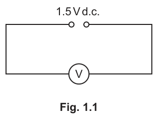
Answer
Voltmeter reading (example):
E = 1.50 V (example)
Background Concept
A voltmeter measures potential difference (p.d.) between two points in a circuit. To measure the p.d. of a supply, the voltmeter must be connected in parallel with the supply terminals. A digital voltmeter has a finite resolution (e.g. 0.01 V), so readings should be recorded to the number of decimal places shown on the display.
Understanding the Question
You are asked to set up the simple circuit with a 1.5 V d.c. source and a voltmeter, then record the reading . The value is whatever your voltmeter shows for the supply (it may be slightly different from 1.50 V).
Approach
- Connect the voltmeter across the supply (in parallel).
- Read once the circuit is connected correctly.
- Record with the unit V and to the meter’s resolution.
Step-by-Step Reasoning
- The voltmeter is connected directly across the 1.5 V d.c. source, so the voltmeter reading is the supply p.d. .
- Read the display and record it with a unit. A typical value is close to .
Key Takeaways
- Voltmeters go in parallel.
- Record to appropriate precision and always include units.
Common Mistakes
- Connecting the voltmeter in series (gives an incorrect/near-zero reading).
- Recording with no unit, or with inconsistent decimal places.
Things to Be Careful About
- Ensure good electrical contact at terminals.
- If the supply is a cell/battery, its open-circuit voltage can be slightly above or below 1.50 V; just record what you observe.
You have been provided with a metre rule with a wire attached. You have also been provided with two identical resistors placed in component holders, each labelled R.
• Set up the circuit shown in Fig. 1.2.
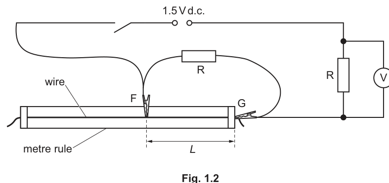
• F and G are crocodile clips.
The distance between F and G is . Attach F and G to the wire so that is approximately .
• Close the switch.
• Record the value of and the voltmeter reading .
= ______
= ______
• Open the switch.
Answer
Example readings (to appropriate precision):
L = 0.317 m, V = 1.04 V (example)
Background Concept
A metre rule allows you to measure a distance along the wire between two crocodile clips. The length is the separation between the contact points of clips F and G. A voltmeter measures the p.d. across the component(s) to which it is connected in parallel.
Understanding the Question
You must build the circuit in Fig. 1.2, set to about , then close the switch and record and the voltmeter reading . Finally, you open the switch.
Approach
- Attach clips F and G so that their separation is approximately .
- Close the switch only while taking readings (to reduce heating changes).
- Read from the metre rule and read from the voltmeter.
Step-by-Step Reasoning
- Place F and G on the wire and measure as the difference between their positions on the metre rule.
- Close the switch and wait briefly for the reading to settle.
- Record from the voltmeter display.
- Open the switch after recording to limit temperature rise in the wire/resistors.
Key Takeaways
- Measure lengths between the actual contact points.
- Take electrical readings with the switch closed only when needed.
Common Mistakes
- Measuring from the wrong reference points (e.g. clip ends rather than contact points).
- Leaving the switch closed continuously (heating changes resistance and affects readings).
Things to Be Careful About
- Record to a sensible precision (typically , i.e. ) and to the voltmeter resolution.
- Ensure clips make firm contact with the wire (oxidation/loose contact increases resistance).
• Write down the value of from (a).
= ______
• Increase by changing the position of F on the wire. Record and and repeat until you have six sets of values of and . Include your values from (b).
Record your results in a table. Include values of in your table.
Answer
Use from (a). Example:
Record at least six sets of and (including (b)) and calculate
Example table (values illustrative):
| 0.317 | 1.04 | 1.45 |
| 0.400 | 1.00 | 1.25 |
| 0.482 | 0.97 | 1.10 |
| 0.589 | 0.94 | 0.951 |
| 0.682 | 0.92 | 0.850 |
| 0.800 | 0.90 | 0.750 |
Table of six (L, V) readings with calculated (E−V)/L (student-dependent; example shown)
Background Concept
In practical work you often measure two quantities and then calculate a third “derived” quantity from them. Here the derived quantity is
where and are in volts and is a length along the wire. If is recorded in metres, then has unit .
Good tables:
- include all readings in one place,
- have clear column headings with quantity symbols and units,
- show consistent precision (same decimal places) within a column.
Understanding the Question
You must:
- Write down the value of from part (a).
- Increase several times, each time recording and the corresponding voltmeter reading .
- Obtain six sets of in total (including your first set from (b)).
- Add a calculated column for .
Approach
- Choose a sensible range of values (e.g. from about up to a larger value, without exceeding the wire length).
- For each :
- close the switch briefly,
- record once stable,
- open the switch.
- After taking measurements, calculate for each row.
Step-by-Step Reasoning
- Record once (from part (a)); use this same value for all rows.
- Generate six data points:
- Start with .
- Move clip F to increase in suitable steps (to produce a good spread of values).
- Fill the table:
- Column 1: with unit (preferably m). Keep a consistent number of decimal places (e.g. 0.001 m).
- Column 2: with unit (V). Keep consistent decimal places (e.g. 0.01 V).
- Calculate derived column for each row:
Example calculation using one row (illustrative numbers):
Key Takeaways
- Use a single, clear results table with headings and units.
- Take enough readings (six) with a good range.
- Show derived quantities calculated correctly and to sensible significant figures.
Common Mistakes
- Forgetting to include the calculated column.
- Missing units in headings, or writing units in the body of the table instead of the heading.
- Inconsistent precision (e.g. mixing 0.3 m and 0.317 m in the same column).
- Not including the data point from part (b) among the six.
Things to Be Careful About
- Use the same value for every calculation.
- Keep the switch closed only while reading to reduce heating.
- Avoid parallax error when reading the metre rule: read with your eye directly above the scale mark at the clip contact point.
Answer
Plot a graph of (in ) on the -axis against (in V) on the -axis.
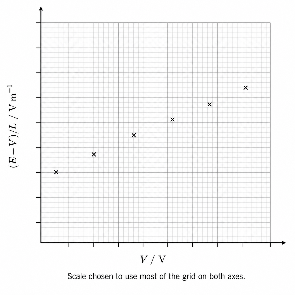
Graph of (E−V)/L against V (see plotting instructions)
Background Concept
A graph is used to reveal whether two quantities are related linearly and to allow constants to be found from the gradient and intercept. Good graph technique includes:
- clear axis labels with units,
- a sensible scale using at least half the grid in each direction,
- accurate plotting with small, neat crosses,
- plotting the correct variables on the correct axes.
Understanding the Question
You must plot on the vertical axis and on the horizontal axis using your six results from (c).
Approach
- Compute for each reading.
- Set up axes: horizontal axis (V), vertical axis ( if in m).
- Choose scales that spread the points well.
- Plot all six points.
Step-by-Step Reasoning
- Decide the range of values (min to max) and the range of .
- Draw axes and label them fully:
- -axis:
- -axis:
- Pick scales (e.g. 1 large square = 0.05 V on , 1 large square = 0.1 on ) so points occupy much of the grid.
- Plot each pair carefully.
Key Takeaways
- Always plot the variables exactly as specified.
- Labels must include both symbol and unit.
Common Mistakes
- Swapping axes (plotting on and on ).
- Missing units in axis labels.
- Choosing a scale that compresses points into a small area.
Things to Be Careful About
- If you used in cm, then is in ; be consistent and label accordingly.
- Use a sharp pencil and plot small crosses; large blobs make best-fit difficult.
Answer
Draw a single straight line of best fit through the plotted points (balanced with roughly equal scatter above and below).
Straight line of best fit drawn
Background Concept
Experimental points usually show scatter due to random uncertainties. A line of best fit is drawn to represent the overall trend. For a linear relationship, it should be a straight line that balances the scatter (roughly equal numbers of points above and below) rather than joining point-to-point.
Understanding the Question
After plotting against , you must draw the straight line that best represents the trend of your data.
Approach
- Use a ruler.
- Position the ruler so the line passes centrally through the cluster of points.
- Do not force the line through the origin unless clearly required by theory (not stated here).
Step-by-Step Reasoning
- Visually assess the pattern of points.
- Place a ruler so that the line has about the same total deviation above and below the line.
- Draw one continuous straight line across most of the graph range.
Key Takeaways
- A best-fit line represents the trend, not a join-the-dots path.
Common Mistakes
- Connecting the points with short segments.
- Drawing a line through all points even when one is clearly anomalous.
- Drawing a line only over a small central section (should extend over the data range).
Things to Be Careful About
- If one point is an outlier, you may still draw the best-fit line for the main cluster; do not automatically force the line to pass through the outlier.
Determine the gradient and -intercept of this line.
gradient = ______
-intercept = ______
Working
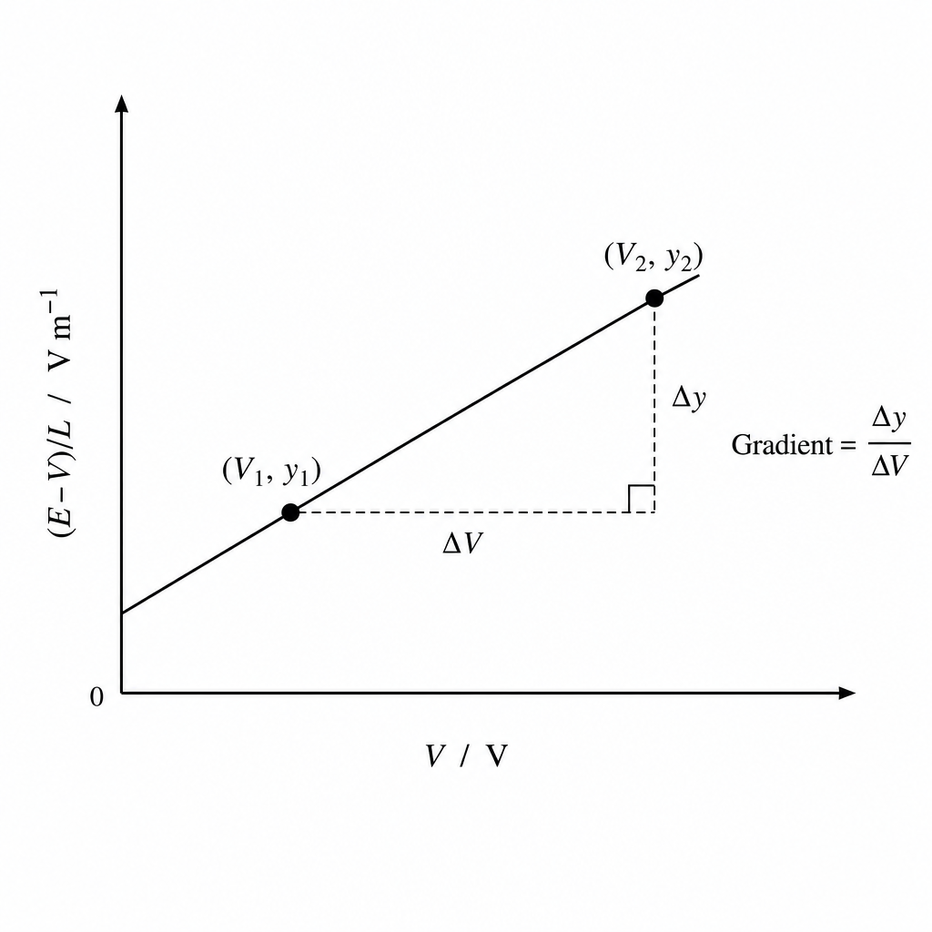
Choose two well-separated points on the best-fit line (example):
Using with :
Answer
gradient = 5.0 m^-1, y-intercept = -3.75 V m^-1 (example)
Background Concept
For a straight-line graph, the equation is
where:
- is the gradient (slope), found from using two points on the line,
- is the -intercept, the value of when .
Using two points that are far apart reduces the percentage uncertainty from reading the graph.
Understanding the Question
You have plotted against and drawn a best-fit line. You must now find:
- the gradient of the best-fit line,
- the -intercept of the best-fit line.
Approach
- Pick two points on the drawn best-fit line (not necessarily your plotted data points), far apart.
- Read their coordinates carefully.
- Compute .
- Find either by reading where the line crosses the -axis, or by substituting one point into .
Step-by-Step Reasoning
- Choose two points far apart on the best-fit line to form a large triangle.
- Read values of from the -axis and from the -axis.
- Calculate gradient:
Units: has units and has units V, so the gradient has units .
4. Find intercept:
- Either read directly at (where the line crosses the -axis),
- Or calculate using with any point on the line.
Key Takeaways
- Use two points on the line, not two experimental points close together.
- Gradient is always .
Common Mistakes
- Using (inverts the gradient).
- Using two plotted points that are too close (large fractional uncertainty).
- Forgetting units for gradient and intercept.
Things to Be Careful About
- Read the coordinates from the line, not from the nearest plotted crosses if they are off the line.
- Keep consistent units: if you plotted in , the gradient unit becomes and intercept becomes .
It is suggested that the quantities and are related by the equation
where and are constants.
Using your answers in (d)(iii), determine the values of and .
Give appropriate units.
= ______
= ______
Working
Given
This matches with and .
So
and
Using (d)(iii) (example):
Answer
P = gradient, Q = −(y-intercept) with units (example: P = 5.0 m^-1, Q = 3.75 V m^-1)
Background Concept
If a graph plots against and the relationship can be written as
then:
- gradient is the coefficient of ,
- intercept is the constant term.
Units come from the fact that and has the same units as .
Understanding the Question
You are given the suggested relationship
You already found the gradient and -intercept from your graph of (on the -axis) against (on the -axis). You must now identify and (with units).
Approach
- Compare the given equation with .
- Read off which constant corresponds to the gradient and which corresponds to the intercept.
- Use the plotted units to determine units of and .
Step-by-Step Reasoning
Let
Then the given equation becomes
So the gradient is and the intercept is .
- Therefore .
- If the -intercept is , then .
Units:
- If is in m, then is in .
- Since is in V,
- And
Key Takeaways
- Gradient gives the coefficient of .
- Intercept sign matters: here the intercept is , not .
- Units follow from the axes.
Common Mistakes
- Taking equal to the -intercept instead of the negative of it.
- Giving incorrect units (e.g. writing in V instead of ).
Things to Be Careful About
- If you used in cm on your table/graph, your and units will be and respectively; do not mix cm-based values with m-based units.
The resistance of R is .
Theory suggests that:
• and are both inversely proportional to
• the graph cuts the -axis at a value of for all values of .
A student repeats the experiment using two identical resistors, each with a lower value of than in the original experiment.
For the student’s experiment, draw a second line on the graph to show the expected results.
Label this line W.
Working
The graph is
Lower gives larger and larger (both ).
The -intercept is where :
So the new line passes through on the -axis, but has a larger gradient (steeper). Since -intercept , it is more negative.
Answer
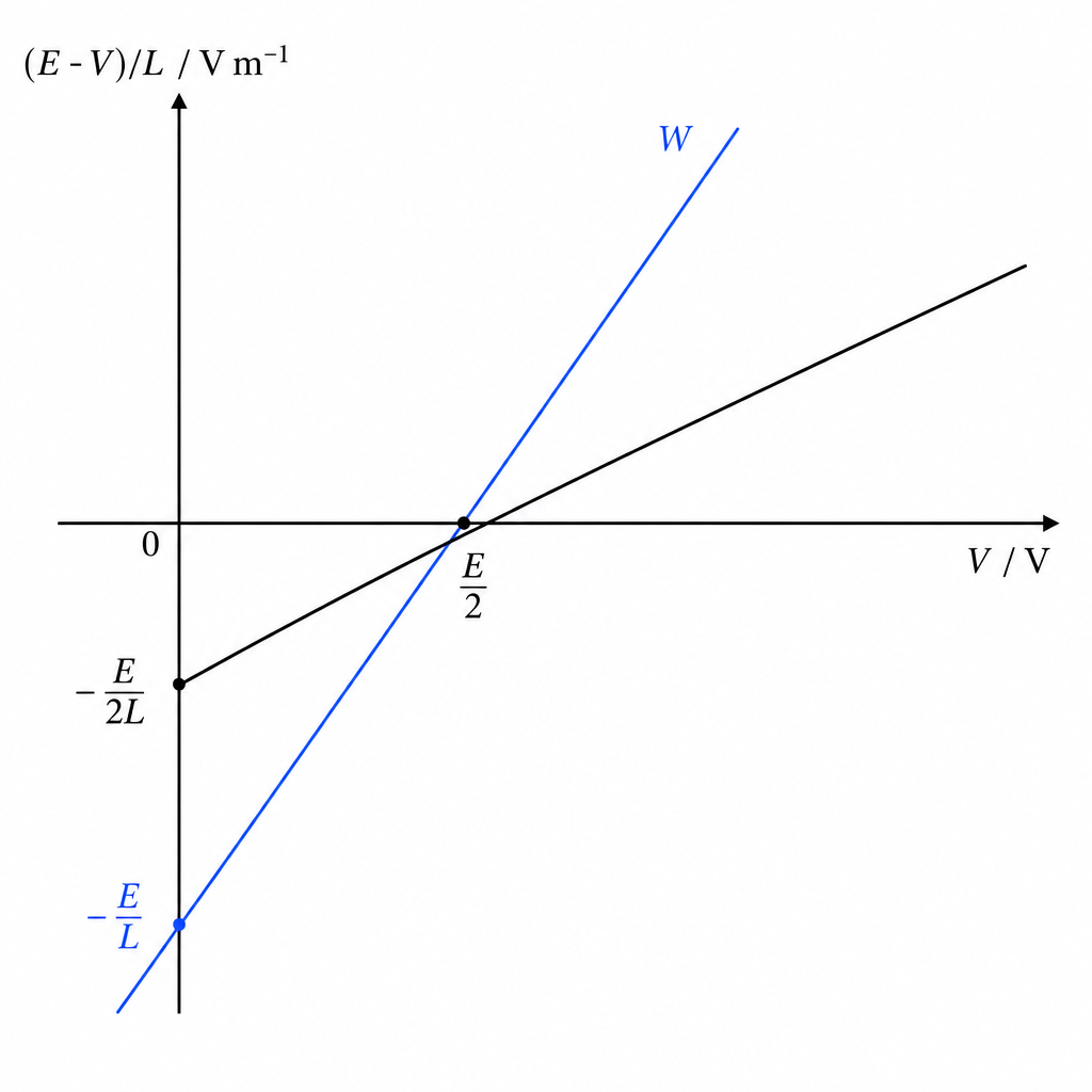
Line W is steeper and pivots about the same x-intercept at V = E/2; y-intercept is more negative.
Background Concept
For a straight line
- gradient ,
- -intercept ,
- -intercept occurs when :
If both and change by the same factor, the ratio stays the same, so the -intercept stays fixed.
Understanding the Question
You are told the theory predictions:
- and are both inversely proportional to ,
- the graph cuts the -axis at for all values of .
A student repeats with smaller resistors (so smaller ). You must draw the expected new line on the same axes and label it W.
Approach
- Work out what happens to the gradient and intercept when decreases.
- Use the given fixed -intercept at .
- Sketch a second straight line consistent with these constraints.
Step-by-Step Reasoning
- Since , decreasing increases , so the line becomes steeper.
- Since , decreasing increases .
- The -intercept is , so increasing makes the -intercept more negative (the line crosses the -axis lower down).
- The -intercept is
If both and increase in the same inverse proportion to , the ratio stays constant, so the line must still cross the -axis at
So the new line W is best thought of as a line that pivots about the fixed point and becomes steeper.
Key Takeaways
- Changing a parameter can change both gradient and intercept.
- A fixed -intercept provides a strong constraint for sketching the new line.
Common Mistakes
- Drawing the new line parallel to the old one (wrong because gradient changes).
- Shifting the -intercept away from (explicitly stated to stay the same).
- Making the -intercept less negative when increases (sign error: intercept is ).
Things to Be Careful About
- Ensure line W is clearly labelled.
- The line should remain straight (same functional form) and should cross the -axis at the same point as the original line.
In this experiment, you will investigate the oscillations of a chain of paper clips.
You have been provided with two spheres of modelling clay.
The diameter of the smaller sphere is , as shown in Fig. 2.1.
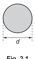
Measure and record .
= ______
Answer
Measure the diameter with a ruler.
Example:
d = 2.40 cm
Background Concept
A measurement should be recorded to the precision allowed by the instrument. For a ruler with 1 mm smallest divisions, the reading resolution is 1 mm, so lengths are typically recorded to the nearest 1 mm (0.1 cm).
Understanding the Question
You are asked to measure the diameter of the smaller modelling-clay sphere (straight line through the centre from one side to the other) and record it.
Approach
Place the sphere against a ruler, view the scale perpendicularly to avoid parallax, and take the diameter as the difference between the two edge readings. Record the result to the nearest 0.1 cm (or 1 mm).
Step-by-Step Reasoning
- Align the sphere so the diameter you measure is the maximum width through the centre.
- Note the ruler reading at one edge of the sphere.
- Note the ruler reading at the opposite edge.
- Subtract to obtain .
- Record to the ruler resolution (typically 0.1 cm).
An acceptable example recording is .
Key Takeaways
- Record to instrument resolution.
- Avoid parallax and misalignment when measuring a diameter.
Common Mistakes
- Writing too many decimal places (e.g. with a ruler).
- Measuring a non-central chord (underestimates the true diameter).
- Parallax error from viewing at an angle.
Things to Be Careful About
- Modelling clay can deform when pressed against the ruler; measure gently.
- Ensure you are measuring the largest width (true diameter).
Estimate the percentage uncertainty in your value of . Show your working.
percentage uncertainty = ______ %
Working
Using a ruler (1 mm resolution), take absolute uncertainty in as .
Example with :
Answer
2.1%
Background Concept
Uncertainty is an estimate of the likely range of values for a measured quantity.
For a ruler:
- smallest division is usually 1 mm.
- a single scale reading is often taken as .
Percentage uncertainty is
Understanding the Question
You must estimate the percentage uncertainty in your measured diameter and show working.
Approach
- Decide the absolute uncertainty in based on the ruler resolution.
- Divide by your measured .
- Multiply by 100 to get a percentage.
Step-by-Step Reasoning
- If the ruler has 1 mm markings, a reasonable uncertainty in a single reading is .
- For example, if :
(If you instead took you would get a larger percentage; the key is that your value must match your stated absolute uncertainty.)
Key Takeaways
- Percentage uncertainty comes from absolute uncertainty divided by the measured value.
- Always show the calculation.
Common Mistakes
- Using instead of without justification.
- Forgetting to multiply by 100.
- Mixing mm and cm in the same calculation.
Things to Be Careful About
- If you measure by subtracting two ruler readings, some students argue for a larger uncertainty (two readings). If you do this, be consistent and show it clearly.
- Quote the final percentage to a sensible number of significant figures (usually 2 s.f.).
• Set up the apparatus as shown in Fig. 2.2.
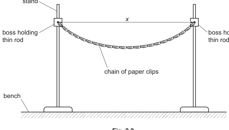
• Ensure that the rods are the same height above the bench.
• Slide the paper clips at the ends of the chain onto the rods.
• The distance between the centres of the rods is .
Position the stands so that is approximately .
• Measure and record .
= ______
Answer
Set the stands so the rod centres are about apart and measure .
Example:
x = 70.0 cm
Background Concept
In practical work, a large part of accuracy is defining exactly what distance you are measuring. Here is the distance between the centres of the rods, so you must identify those centres consistently.
Understanding the Question
You must set up the chain between two rods at the same height and measure the centre-to-centre separation , with .
Approach
- Build the apparatus as shown.
- Adjust the stands until the separation is roughly 70 cm.
- Measure with a ruler/tape measure between the centres of the rods.
- Record with an appropriate unit and precision.
Step-by-Step Reasoning
- Ensure rods are at equal height to avoid twisting the chain.
- Use a metre rule or tape measure parallel to the bench.
- Identify the centre of each rod (e.g. halfway across its diameter) and measure between these centres.
- Record as, for example, (nearest 0.1 cm if using mm divisions).
Key Takeaways
- Measure exactly what is defined (centre-to-centre).
- Record the unit clearly.
Common Mistakes
- Measuring between the inner edges or outer edges of rods (not the centres).
- Forgetting the unit (cm).
- Allowing the ruler to be at an angle (gives a longer distance).
Things to Be Careful About
- Parallax: view the scale straight on.
- If the rod diameter is not negligible, you must account for it to get centre-to-centre distance.
• Use the hook to attach the smaller sphere of modelling clay to the chain of paper clips as shown in Fig. 2.3.
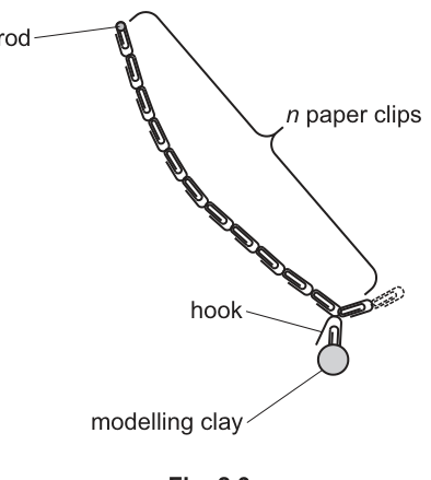
• The number of paper clips between the hook and the end of the chain is , as shown in Fig. 2.3.
Place the hook so that is 11.
• Calculate , where
Give your answer to three significant figures.
= ______
Working
With :
Answer
4.95
Background Concept
Cube roots and indices are interchangeable:
The instruction “three significant figures” means you round the final numerical value so it has 3 non-zero digits.
Understanding the Question
You are told to place the hook so that paper clips, then calculate
with the final answer to 3 s.f.
Approach
Compute , then take the cube root, then round.
Step-by-Step Reasoning
- Square :
- Take the cube root:
- Round to 3 s.f.:
Key Takeaways
- Recognise as .
- Round only at the end.
Common Mistakes
- Calculating instead of the cube root.
- Rounding too early, then using the rounded value in later calculations.
- Giving 2 s.f. or 4 s.f. instead of 3 s.f.
Things to Be Careful About
- Write enough digits in intermediate working to avoid rounding error before the final step.
• Pull the sphere towards you through a short distance. When the sphere is released, it will oscillate.
• Take measurements to determine the period of these oscillations.
= ______
Working
Time oscillations twice and average.
Example:
Answer
T = 1.20 s
Background Concept
The period is the time for one complete oscillation. A stopwatch has reaction-time uncertainty (often ~0.2 s for a single start/stop), so timing just one oscillation gives a large percentage uncertainty.
A standard method is:
- time oscillations (e.g. or ),
- then divide by :
Repeating and averaging reduces random uncertainty.
Understanding the Question
You must “take measurements to determine the period ” of the oscillating clay sphere on the paper-clip chain.
Approach
- Choose a clear reference point (e.g. centre position).
- Time a large number of oscillations.
- Repeat the timing.
- Average and divide by the number of oscillations to obtain .
Step-by-Step Reasoning
- Displace the sphere a small distance and release so it oscillates with small amplitude.
- Start the stopwatch as the sphere passes the reference point in a chosen direction.
- Count 10 complete oscillations and stop the watch when it returns to the same point moving in the same direction.
- Repeat the timing.
- Example:
Key Takeaways
- Time many oscillations to reduce percentage uncertainty.
- Repeat and average to reduce random error.
Common Mistakes
- Timing only one oscillation.
- Not using the same reference point/direction for start and stop.
- Counting oscillations incorrectly (e.g. counting half-oscillations).
Things to Be Careful About
- Keep amplitude small; large amplitudes can change the period and cause the motion to become irregular.
- If the oscillations decay (damping), take timings early and consistently.
• Roll the two spheres into one larger sphere.
• Measure and record the diameter of the larger sphere.
= ______
• Repeat (b) and (c) with a value of approximately and with the hook placed so that is 7.
= ______
= ______
= ______
Working
Example readings after combining spheres:
With :
Timing oscillations (example ):
Answer
d = 3.02 cm, x = 80.0 cm, N = 3.66, T = 1.02 s
Background Concept
This part repeats the same measurement and timing skills:
- measure lengths (, ) to the instrument resolution,
- compute a derived quantity from the given formula,
- measure period by timing multiple oscillations and dividing.
Understanding the Question
You must:
- Combine the two clay spheres into one larger sphere and measure its diameter .
- Re-set the apparatus with .
- Place the hook so and calculate .
- Measure the period of oscillation again.
Approach
Follow the same methods used earlier:
- diameter with ruler (or calipers if available),
- measured centre-to-centre,
- compute and round to 3 s.f. if needed,
- time 10–20 oscillations and divide to get .
Step-by-Step Reasoning
- Roll the clay into a sphere; because clay deforms, rotate it and check several diameters, then take a representative value.
- Measure as the centre-to-centre separation.
- With :
- For the period, choose a number of oscillations such as 10, measure time , then
Repeat and average if possible.
Key Takeaways
- Consistency: use the same measurement definitions (centre-to-centre, full oscillations) each time.
- Derived quantities must be rounded appropriately.
Common Mistakes
- Forgetting to change to 7.
- Using instead of .
- Measuring between rod edges rather than centres.
Things to Be Careful About
- The larger sphere may be less spherical; this increases uncertainty in .
- Ensure rods remain at equal height; otherwise the motion can become irregular and affect .
It is suggested that the relationship between , , and is
where is a constant.
Using your data, calculate two values of .
first value of = ______
second value of = ______
Working
From
Using SI units.
Run 1 (example): , , ,
Run 2 (example): , , ,
Answer
first value of :
second value of :
k1 = 5.94 s^2 m, k2 = 6.03 s^2 m
Background Concept
If a relationship is correct, a constant calculated from different experimental runs should agree within experimental uncertainty.
From
we rearrange to calculate :
You must use consistent units for and (both in m, or both in cm). The numerical value (and unit) of depends on that choice.
Understanding the Question
You have two sets of data (small sphere run and large sphere run). You must calculate for each run to obtain two values, then you can later judge agreement.
Approach
- Make the subject.
- For each run, substitute , , , .
- Compute and record to a sensible number of significant figures.
Step-by-Step Reasoning
- Rearrangement:
- Substitute Run 1 values (example): square and carefully, then divide by .
- Repeat for Run 2.
A good check is that if the relationship holds, the two values should be similar (not identical).
Key Takeaways
- Rearranging is essential: isolate the constant.
- Consistent units are critical when calculating derived constants.
Common Mistakes
- Forgetting to square or .
- Mixing cm and m for and .
- Using rounded too aggressively (can shift ).
Things to Be Careful About
- Quote to appropriate significant figures based on your least precise measurement.
- Include the unit of if you used SI units (here ).
Answer
is calculated from measured , and .
Since , and are recorded to about 3 significant figures, should be given to 3 significant figures (not more).
k to 3 s.f., limited by T, x and d
Background Concept
For calculated quantities, the number of significant figures should reflect the precision of the input data. A derived value cannot be justified to more significant figures than the least precise measurement used to compute it.
Understanding the Question
You must explain why you chose the number of significant figures used when you reported your two values of .
Approach
- Identify which measured quantities go into .
- Identify the least precise (fewest significant figures / largest percentage uncertainty).
- State that should be quoted to match that limiting precision.
Step-by-Step Reasoning
- The calculation is
- is given to 3 s.f. by instruction.
- and are typically recorded from a ruler/tape to about 3 s.f. (e.g. , ).
- from timing multiple oscillations is usually recorded to about 3 s.f. (e.g. ).
Therefore it is reasonable to quote to 3 s.f. Quoting 4 s.f. would suggest a precision not supported by the measurements.
Key Takeaways
- Significant figures for a derived result must reflect measurement precision.
Common Mistakes
- Copying all calculator digits.
- Using inconsistent significant figures between the two values.
Things to Be Careful About
- The true limiting factor is often percentage uncertainty (stopwatch reaction time can dominate), so in many real datasets 2–3 s.f. is the maximum justifiable range.
It is suggested that the percentage uncertainty in the values of is 15%.
Using this uncertainty, explain whether your results support the relationship in (e).
Working
Using example values and :
Since , the values agree within the uncertainty.
Answer
Yes. The two values of are consistent within , so the results support the relationship.
Yes, consistent within 15%.
Background Concept
To test whether two results agree within an uncertainty, you compare their difference with the allowed uncertainty range.
If the percentage uncertainty in is , then two values of should typically differ by no more than about (order-of-magnitude check) to be considered consistent.
A common quantitative check is percentage difference:
Understanding the Question
You are told to assume a uncertainty in and decide whether your experimental results support the proposed relationship.
Approach
- Compute how far apart the two values are (as a percentage).
- Compare this with .
- State a clear conclusion (supports / does not support).
Step-by-Step Reasoning
- Using example values:
- Because is much less than , the two values are consistent within the stated uncertainty.
- Therefore the experimental results support the relationship.
Key Takeaways
- “Support” means agreement within uncertainty, not perfect equality.
Common Mistakes
- Comparing absolute difference without considering the size of the values.
- Using of the larger value but not stating what you did.
- Giving a conclusion without referencing the uncertainty.
Things to Be Careful About
- If your two values differ by more than , you should say results do not support (within that uncertainty) and could mention experimental limitations as a possible reason.
Describe four sources of uncertainty or limitations of the procedure for this experiment.
For any uncertainties in measurement that you describe, you should state the quantity being measured and a reason for the uncertainty.
Answer
- Uncertainty in : stopwatch reaction time and difficulty judging the instant the sphere passes a fixed reference point.
- Uncertainty in : oscillations may not stay in one vertical plane (twisting of the chain), so the motion is not perfectly periodic.
- Uncertainty in : difficult to measure centre-to-centre of the rods accurately; parallax and uncertainty in locating the rod centres.
- Uncertainty in : modelling clay is not a perfect rigid sphere and can deform, so the measured diameter depends on orientation/pressure.
Four limitations/uncertainties listed (T reaction time; non-planar oscillation; x centre-to-centre; d deformation).
Background Concept
A good evaluation point:
- names the quantity affected (e.g. , , ),
- states why it is uncertain (instrument limits, human judgement, motion not ideal),
- indicates whether it is random (varies trial-to-trial) or systematic (bias).
Understanding the Question
You must give four sources of uncertainty or limitations in this procedure. For measurement uncertainties, you must state the quantity and the reason.
Approach
Look at each measured or controlled quantity in the experiment (, , /, , and the oscillation conditions) and identify what makes it hard to measure reliably or what makes the model imperfect.
Step-by-Step Reasoning
Four strong, creditworthy examples are:
- Period (reaction time / judgement): starting and stopping a stopwatch depends on human reaction time, and it is hard to decide the exact moment the sphere passes the reference position.
- Period (non-ideal motion): the chain can twist so the sphere oscillates in an ellipse or with coupled modes rather than a single simple oscillation, so the period is not constant.
- Distance (definition of centres): is defined as centre-to-centre of rods; the centre is not a sharp point on the apparatus, giving reading uncertainty and possible parallax.
- Diameter (deformation): modelling clay is compressible and may not form a perfect sphere; pressing it against a ruler can change its size slightly, and different orientations give different diameters.
Other acceptable limitations (if distinct) could include damping (amplitude decays, making later oscillations harder to time) or inconsistency in release (not releasing from same displacement).
Key Takeaways
- Evaluation marks come from specific, physics-based limitations tied to the measurements.
Common Mistakes
- Vague statements like “human error” without naming the quantity or cause.
- Repeating the same point (e.g. reaction time) in different words.
- Stating an improvement instead of a limitation (belongs in part (g)(ii)).
Things to Be Careful About
- Ensure each of the four points is genuinely different.
- For measurement uncertainty, always include both: the measured quantity and why it is uncertain.
Describe four improvements that could be made to this experiment. You may suggest the use of other apparatus or different procedures.
Answer
- Improve measurement: use a video camera / motion sensor and determine from playback or data logging instead of a stopwatch.
- Improve measurement: time a larger number of oscillations (e.g. 20) and repeat several times, then average.
- Improve measurement: mark the rod centres and measure with a set square/metre rule aligned horizontally to reduce parallax and improve centre-to-centre accuracy.
- Improve measurement: use vernier calipers and measure several diameters at different orientations, then take the mean.
Four improvements listed (data-logged T; more oscillations and repeats; better x measurement; better d measurement).
Background Concept
Improvements should be specific and should reduce the uncertainties/limitations identified. Good improvements either:
- reduce random uncertainty (repeat/average, better timing method),
- reduce systematic error (better definition of measurement points),
- make the motion closer to the ideal model (reduce twisting/damping effects).
Understanding the Question
You must describe four improvements (apparatus or procedure changes) that would make the experiment more reliable/accurate.
Approach
For each main limitation (timing, geometry measurement, non-ideal sphere), propose a concrete change and briefly state how it helps.
Step-by-Step Reasoning
- Replace stopwatch timing of : use video analysis or a motion sensor/data logger to find the period from recorded position-time data; this removes reaction-time error.
- Reduce random uncertainty in : time 20 oscillations rather than 10 and repeat multiple trials; average the calculated periods.
- Measure more accurately: mark the centres of rods and use a rigid metre rule aligned at the same height; using a set square helps align the rule and reduces parallax.
- Measure more accurately: use vernier calipers and measure several diameters at different orientations; average to reduce the effect of non-sphericity.
Other possible improvements include ensuring oscillations stay in one plane (guides or preventing twist) and ensuring the stands/rods are level using a spirit level.
Key Takeaways
- Improvements must be practical and linked to identifiable uncertainties.
Common Mistakes
- Saying “use more accurate equipment” without naming it.
- Giving improvements that do not address a real limitation in the experiment.
- Repeating the same improvement (e.g. “repeat readings”) for multiple marks without adding new detail.
Things to Be Careful About
- Keep improvements distinct.
- Make sure each improvement is described clearly enough that an experimenter could implement it.