Physics 9702/32 — May/June 2025

Cambridge AS Level · Advanced Practical Skills · worked solutions for every part, with the mark scheme

questions

marks

120

minutes

Topics Manipulation, Measurement and Observation · Presentation of Data and Observations · Analysis, Conclusions and Evaluation

Q1MediumManipulation, Measurement and ObservationPresentation of Data and ObservationsAnalysis, Conclusions and Evaluation

In this experiment, you will investigate a light-dependent resistor (LDR).

(a)

• Connect the circuit shown in Fig. 1.1.

Fig. 1.1

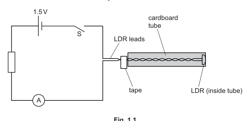
• Ensure that the switch S is open.

• Slide the LDR leads into the tube until the front of the LDR is just level with the open end of the tube, as shown in Fig. 1.1.

• With the LDR in this position, attach a piece of adhesive tape to the leads as a marker at the other end of the tube, as shown in Fig. 1.1.

• Slide the tube until the LDR is approximately half-way along it, as shown in Fig. 1.2.

Fig. 1.2

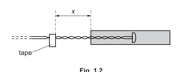
• The distance between the tape and the tube is $x$ .

Measure and record $x$ .

$x$ = ______

• Close S and record the ammeter reading $I$ .

$I$ = ______

• Open S.

2M Similar

DifficultyEasy

Worked solution

Answer

(Example readings)

$x = 10.0\ \text{cm}$

$I = 0.27\ \text{mA}$

Final answer

Example: x = 10.0 cm, I = 0.27 mA

Detailed explanation

Background Concept

An LDR (light-dependent resistor) has a resistance that depends on the light intensity falling on it. In a simple series circuit, changing the LDR resistance changes the circuit current $I$ . Placing the LDR inside a tube changes how much light reaches it (the tube shields it), so moving it to different positions changes $I$ .

Understanding the Question

You are told to set up the circuit and place the LDR in a defined position inside the tube. You then measure the separation $x$ (a distance between the tape marker and the end of the tube) and record the ammeter reading $I$ when the switch $S$ is closed.

The marks here are mainly for:

a sensible value of $x$ with suitable precision and unit,
a sensible value of $I$ with suitable precision and unit.

Approach

Set up the circuit exactly as shown and keep the switch open until you are ready to take the current reading.
Measure $x$ with a ruler (use mm divisions if available), and record $x$ with consistent precision.
Close the switch briefly, allow the reading to settle, read $I$ from the ammeter, record it, then open the switch again.

Step-by-Step Reasoning

When measuring $x$ , ensure the ruler is aligned parallel to the leads/tube direction and your eye is directly above the scale to avoid parallax.
Record $x$ to the resolution of the ruler (typically nearest $0.1\ \text{cm}$ if mm markings are used).
For $I$ , choose the correct meter range if the ammeter is not auto-ranging. Read the scale carefully, estimate between divisions if required, and record to a consistent number of decimal places that matches the instrument resolution.
Open the switch after taking the reading to reduce heating effects and battery drain, which can cause drift.

Key Takeaways

Record raw measurements with appropriate precision and units.
Good practice: switch closed only while measuring to keep conditions stable.

Common Mistakes

Omitting units (e.g. writing $10.0$ instead of $10.0\ \text{cm}$ ).
Recording $x$ with unrealistic precision (e.g. $10.00\ \text{cm}$ using a simple ruler).
Parallax error when reading the ruler or analog ammeter.

Things to Be Careful About

Ensure the tape marker position is fixed before measuring $x$ .
Wait for the ammeter reading to stabilise (LDR response can take a short time).
Keep ambient lighting roughly constant while taking readings.

Techniques used

set up the circuit as shown and check the switch position before taking readingstake a length measurement with an appropriate ruler precisionread an ammeter at eye level and record the value to a suitable resolution

(b)

Change $x$ by moving the LDR to a new position inside the tube, with $x$ in the range $4\ \text{cm}$ to $18\ \text{cm}$ . Record $x$ and $I$ .

Repeat until you have six sets of values of $x$ and $I$ .

Record your results in a table. Include values of $\sqrt{I}$ in your table.

10M Similar

DifficultyMedium

Worked solution

Answer

A single table with at least six sets of readings of $x$ and $I$ (with $4\ \text{cm} \le x \le 18\ \text{cm}$ ) and calculated values of $\sqrt{I}$ .

(Example set of results)

$x / \text{cm}$	$I / \text{mA}$	$\sqrt{I} / \text{mA}^{1/2}$
4.0	0.58	0.76
7.0	0.41	0.64
10.0	0.27	0.52
13.0	0.16	0.40
16.0	0.078	0.28
18.0	0.040	0.20

Final answer

Table of x, I and sqrt(I) with six readings (example shown).

Detailed explanation

Background Concept

In this experiment, you are investigating how the current $I$ in a circuit changes when the LDR is moved inside a tube. The tube reduces the light intensity reaching the LDR as it is moved further from the open end, changing the LDR resistance and therefore changing $I$ .

You are also asked to compute $\sqrt{I}$ for each reading. This is often done because many relationships become linear when you transform a variable (e.g. plotting $\sqrt{I}$ against $x$ might produce a straight line).

Understanding the Question

You must:

choose new positions of the LDR so that $x$ spans the given range $4\ \text{cm}$ to $18\ \text{cm}$ ,
record six pairs of values $(x, I)$ ,
present all data in one clear table,
include a calculated column for $\sqrt{I}$ .

The marks are typically for: sufficient range, enough points (six), correct table layout (headings with units), and correct calculation and sensible rounding of $\sqrt{I}$ .

Approach

Decide six values of $x$ spread across $4$ to $18\ \text{cm}$ (not clustered).
For each $x$ , measure $x$ and record it, then close the switch and record $I$ .
Calculate $\sqrt{I}$ for each row.
Ensure consistent decimal places/precision in each column.

Step-by-Step Reasoning

Choosing values of $x$ : Use an even spread (e.g. approximately every $2$ to $3\ \text{cm}$ ) to improve the quality of any graph you later plot.
Taking readings: Keep ambient light conditions as constant as possible (same room lighting, avoid shadows from your body). Close the switch only long enough to take the reading.
Recording $x$ : If your ruler reads to $1\ \text{mm}$ , record $x$ to the nearest $0.1\ \text{cm}$ . Use the same precision for all $x$ values.
Recording $I$ : Record to the resolution of the ammeter. If digital, copy all displayed digits that are stable.
Calculating $\sqrt{I}$ :
- Use the same unit for $I$ throughout the table.
- If you keep $I$ in mA, then $\sqrt{I}$ has units $\text{mA}^{1/2}$ .
- Round $\sqrt{I}$ sensibly (usually to the same number of significant figures as $I$ , or consistent decimal places across the $\sqrt{I}$ column).

Key Takeaways

Collect enough data over a wide enough range to reveal a relationship.
Present data in one well-formatted table with headings and units.
Derived quantities must be calculated correctly and recorded consistently.

Common Mistakes

Using fewer than six sets of readings.
Not spanning the range $4\text{ to }18\ \text{cm}$ .
Missing units in table headings (units should be in the header, not repeated in every cell).
Calculating $\sqrt{I}$ using inconsistent units (mixing A and mA between rows).

Things to Be Careful About

Keep the number of decimal places consistent within a column.
Don’t write $\sqrt{I}$ values with excessive precision if $I$ is only measured roughly.
If the current fluctuates, wait for it to settle or take repeat readings and use a mean (and record consistently).

Techniques used

vary the independent variable over a suitable range and take multiple readingsrecord results in a single table with correct headings and unitscalculate a derived quantity from measured data with consistent significant figures

(c)

(i)

Plot a graph of $\sqrt{I}$ on the $y$ -axis against $x$ on the $x$ -axis.

3M Similar

DifficultyMedium-Easy

Worked solution

Answer

Graph plotted of $\sqrt{I}$ (y-axis) against $x$ (x-axis), with axes labelled $x / \text{cm}$ and $\sqrt{I} / \text{mA}^{1/2}$ , suitable scales, and all points plotted.

Final answer

Graph of sqrt(I) vs x plotted.

Detailed explanation

Background Concept

A graph is used to display how one variable depends on another. Here, $x$ is the independent variable (you choose it), so it goes on the x-axis. $\sqrt{I}$ depends on $x$ , so it goes on the y-axis.

Good graphing technique is assessed: clear labels, sensible scales, accurate plotting.

Understanding the Question

You must plot $\sqrt{I}$ against $x$ using your table from (b). The examiner expects:

correct choice of axes,
axes labelled with quantities and units,
a scale that uses at least half (preferably most) of the available grid,
points plotted accurately.

Approach

Put $x$ on the horizontal axis and $\sqrt{I}$ on the vertical axis.
Choose scales that make the plotted points spread widely.
Plot each pair $(x, \sqrt{I})$ as a small cross or dot with a circle.

Step-by-Step Reasoning

c-i-graph-axes

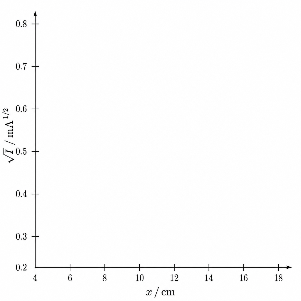
Axis labels: Write labels in the form quantity / unit, e.g. $x / \text{cm}$ and $\sqrt{I} / \text{mA}^{1/2}$ .
Scale choice: Avoid awkward scales (e.g. 3 squares = 1 unit). Choose something like 1 large square = 1 cm or 2 cm, depending on your range.
Plotting points: Use a sharp pencil. Plot to the nearest half small square. Make sure each point is clearly visible but not oversized.

Key Takeaways

Independent variable on x-axis, dependent variable on y-axis.
Correct labels and scales are as important as the points.

Common Mistakes

Swapping axes (plotting $x$ on y-axis).
Missing units or writing units incorrectly.
Choosing a scale that compresses points into a small area.

Things to Be Careful About

Keep the same units you used in the table (don’t switch from mA to A unless you recompute $\sqrt{I}$ ).
Start axes at zero unless doing so wastes most of the grid; if you use a non-zero origin, it must be clearly indicated.

Techniques used

choose appropriate axes and scales to use most of the graph gridlabel axes with quantity and unitplot points accurately with suitable markers

(ii)

Draw the straight line of best fit.

1M Similar

(iii)

Determine the gradient and $y$ -intercept of this line.

gradient = ______

$y$ -intercept = ______

2M Similar

DifficultyMedium

Worked solution

Working

Using two points on the best-fit line, e.g. $(x,\sqrt{I}) = (4.0\ \text{cm}, 0.76\ \text{mA}^{1/2})$ and $(18.0\ \text{cm}, 0.20\ \text{mA}^{1/2})$ :

\text{gradient} = \frac{\Delta y}{\Delta x} = \frac{0.20 - 0.76}{18.0 - 4.0} = -0.040\ \text{mA}^{1/2}\ \text{cm}^{-1}

\text{y-intercept } b = y - mx = 0.76 - (-0.040)(4.0) = 0.92\ \text{mA}^{1/2}

Answer

$\text{gradient} = -0.040\ \text{mA}^{1/2}\ \text{cm}^{-1}$

$\text{y-intercept} = 0.92\ \text{mA}^{1/2}$

Final answer

gradient = -0.040 mA^(1/2) cm^-1, y-intercept = 0.92 mA^(1/2)

Detailed explanation

Background Concept

For a straight-line graph, the gradient (slope) is defined by

\text{gradient} = \frac{\Delta y}{\Delta x}

and the y-intercept is the value of $y$ when $x = 0$ . If the graph is of the form $y = mx + c$ , then:

gradient $m$ tells you how much $y$ changes per unit change in $x$ ,
intercept $c$ is the value of $y$ at $x = 0$ .

Understanding the Question

You have a graph of $y = \sqrt{I}$ against $x$ . You must determine:

the gradient of the best-fit straight line,
the y-intercept of that line.

These values come from the line, not from individual data points (unless a data point lies exactly on the line).

Approach

Choose two points on the best-fit line that are far apart (to reduce percentage reading error).
Read their coordinates accurately.
Compute gradient using $\Delta y/\Delta x$ .
Find y-intercept by reading where the line crosses the y-axis, or by substituting one point into $y = mx + c$ .

Step-by-Step Reasoning

Choosing points: Use intersections with grid lines if possible to improve accuracy.
Gradient:
- Compute $\Delta y$ as (upper point y) minus (lower point y).
- Compute $\Delta x$ as (right point x) minus (left point x).
- Divide to get gradient, and include units: (units of $y$ ) per (units of $x$ ).
Sign: If the line slopes downwards as $x$ increases, the gradient is negative.
Intercept:
- Reading method: extend the line to $x=0$ and read $y$ .
- Calculation method: rearrange $y = mx + c$ to $c = y - mx$ .

Key Takeaways

Always use points on the best-fit line and make a large triangle.
Gradient is $\Delta y/\Delta x$ , not $y/x$ .
Quote units and sign correctly.

Common Mistakes

Using two experimental points that are not on the best-fit line.
Using small separations (gives large percentage uncertainty).
Inverting the gradient as $\Delta x/\Delta y$ .
Forgetting the negative sign for a downward slope.

Things to Be Careful About

Ensure you read coordinates to the precision allowed by the graph scale.
Keep the same units as your axis labels when stating gradient/intercept.
If your axes use cm, your gradient unit includes $\text{cm}^{-1}$ (unless you convert to m consistently).

Techniques used

use two widely separated points on the best-fit line to calculate a gradientcalculate gradient as \Delta y / \Delta x with correct unitsdetermine the y-intercept by reading from the graph or using y = mx + c

(d)

It is suggested that the quantities $I$ and $x$ are related by the equation

\sqrt{I} = ax + b

where $a$ and $b$ are constants.

Using your answers in (c)(iii), determine the values of $a$ and $b$ .
Give appropriate units.

$a$ = ______

$b$ = ______

2M Similar

DifficultyMedium-Easy

Worked solution

Working

Given

\sqrt{I} = ax + b

Comparing with $y = mx + c$ for a graph of $y = \sqrt{I}$ against $x$ :

a = \text{gradient}, \qquad b = \text{y-intercept}

Answer

a = -0.040\ \text{mA}^{1/2}\ \text{cm}^{-1}

b = 0.92\ \text{mA}^{1/2}

Final answer

a = -0.040 mA^(1/2) cm^-1, b = 0.92 mA^(1/2)

Detailed explanation

Background Concept

If experimental data gives a straight-line graph, it can be compared to the standard linear form:

y = mx + c

where $m$ is the gradient and $c$ is the y-intercept. Any equation that can be written in this form allows you to identify constants directly from the graph.

Units:

If $y$ has units $[y]$ and $x$ has units $[x]$ , then the gradient has units $[y]/[x]$ .
The y-intercept has the same units as $y$ .

Understanding the Question

You are given the suggested relationship:

\sqrt{I} = ax + b

You already found the gradient and intercept of the graph of $\sqrt{I}$ (y-axis) against $x$ (x-axis). You must use those graph values to find $a$ and $b$ , including appropriate units.

Approach

Identify $\sqrt{I}$ as $y$ and $x$ as $x$ .
Compare directly with $y = mx + c$ .
Therefore $a$ corresponds to the gradient and $b$ to the intercept.
Assign units from the axis units used on your graph.

Step-by-Step Reasoning

From

\sqrt{I} = ax + b

we can see it is already linear in $x$ .

On a plot of $\sqrt{I}$ $I$ vs $x$ $x$ :
- gradient $= a$ ,
- y-intercept $= b$ .
Units:
- If $\sqrt{I}$ was plotted in $\text{mA}^{1/2}$ and $x$ in cm, then

[a] = \frac{\text{mA}^{1/2}}{\text{cm}} = \text{mA}^{1/2}\ \text{cm}^{-1}

and

[b] = \text{mA}^{1/2}.

Key Takeaways

Comparing your graph equation to $y = mx + c$ lets you read constants as gradient/intercept.
Units for constants come directly from the plotted quantities.

Common Mistakes

Giving $a$ the same units as $\sqrt{I}$ (it must include per cm or per m).
Converting $x$ to metres for the unit but not converting the numeric gradient value (units and numbers must be consistent).
Swapping $a$ and $b$ .

Things to Be Careful About

Use the same unit system you used on the graph when stating units for $a$ and $b$ .
Quote $a$ with the correct sign (often negative here because current decreases as $x$ increases).

Techniques used

match a linear equation to the straight-line graph formidentify constants as gradient and interceptdetermine appropriate units for constants from axis units

Q2MediumManipulation, Measurement and ObservationAnalysis, Conclusions and EvaluationPresentation of Data and Observations

In this experiment, you will investigate the elastic properties of rubber cord.

(a)

(i)

You are provided with a wire with a clip and two slotted masses attached, as shown in Fig. 2.1.

Fig. 2.1

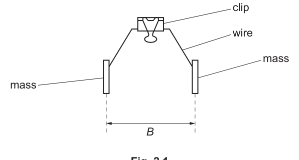
The distance between the centres of the two slotted masses is $B$ , as shown in Fig. 2.1.

Measure and record $B$ .

$B$ = ______

1M Similar

DifficultyEasy

Worked solution

Answer

Measure the distance between the centres of the two slotted masses with a ruler.

Example recorded value:

B = 8.20\ \text{cm}

Final answer

B = 8.20 cm (example)

Detailed explanation

Background Concept

In Paper 3, marks for a measurement usually depend on using an appropriate instrument and recording the value to a realistic precision. A metre rule / ruler typically has 1 mm smallest division, so lengths are usually recorded to the nearest 1 mm (or 0.1 cm).

Understanding the Question

You are given a wire with two slotted masses attached. The quantity $B$ is the distance between the centres of the two masses (as indicated in the diagram). You must measure $B$ and record it.

Approach

Identify the centre of each mass (use the symmetry of the cylindrical slotted mass).
Use a ruler placed close and parallel to the line joining the centres.
Read $B$ at eye level to reduce parallax.
Record with sensible precision (e.g. nearest 1 mm).

Step-by-Step Reasoning

Place the ruler so that its scale is as close as possible to the masses.
Align the ruler along the horizontal separation between the centres.
Read the position of the centre of one mass and the centre of the other mass; take the difference to obtain $B$ .
Record $B$ to the nearest 1 mm (or 0.1 cm). For example:

B = 8.20\ \text{cm}

Key Takeaways

Measurements must match the instrument resolution.
Parallax and ambiguous reference points are major contributors to uncertainty.

Common Mistakes

Measuring edge-to-edge instead of centre-to-centre.
Recording too many decimal places (unrealistic precision).
Reading the ruler from an angle (parallax error).

Things to Be Careful About

Ensure you are measuring the correct distance (centre lines, not outer edges).
Keep the ruler parallel to $B$ and as close as possible to reduce alignment error.
Record units clearly (cm or mm).

Techniques used

measure a length with a ruler while avoiding parallaxtake readings between defined reference pointsrecord a measurement to appropriate precision

(ii)

Estimate the percentage uncertainty in your value of $B$ . Show your working.

percentage uncertainty = ______ $\%$

1M Similar

DifficultyMedium-Easy

Worked solution

Working

Using a ruler (1 mm divisions), take uncertainty in each centre position as $\pm 1\ \text{mm}$ .

So uncertainty in $B$ (difference of two readings):

\Delta B \approx \pm 2\ \text{mm} = \pm 0.2\ \text{cm}

For $B = 8.20\ \text{cm}$ ,

\%\ \text{uncertainty} = \frac{0.2}{8.20}\times 100 = 2.4\%

Answer

\text{percentage uncertainty} \approx 2.4\%

Final answer

2.4% (example)

Detailed explanation

Background Concept

Percentage uncertainty tells you how large the absolute uncertainty is compared to the measured value:

\%\ \text{uncertainty} = \frac{\Delta x}{x} \times 100

For a ruler, a single reading is typically uncertain by about half to one smallest division, depending on how hard it is to judge the reference point. When a length is found by subtracting two readings, the absolute uncertainties from each end add.

Understanding the Question

You must estimate the percentage uncertainty in your measured $B$ , and show working. You are expected to:

state an absolute uncertainty for $B$ based on your measuring method, then
convert it into a percentage.

Approach

Decide the absolute uncertainty in each endpoint reading (based on ruler resolution and how well the centre can be judged).
Add the endpoint uncertainties to get $\Delta B$ .
Use $\% = (\Delta B / B) \times 100$ .

Step-by-Step Reasoning

If the ruler has 1 mm divisions, a cautious estimate for each centre reading might be $\pm 1\ \text{mm}$ (the centre is not a sharp point).
Because $B$ comes from the difference of two readings, the worst-case absolute uncertainty is approximately:

\Delta B \approx 1\ \text{mm} + 1\ \text{mm} = 2\ \text{mm}

Convert to the same unit as $B$ (e.g. $2\ \text{mm} = 0.2\ \text{cm}$ ).
Then compute:

\%\ \text{uncertainty} = \frac{0.2}{8.20}\times 100 = 2.4\%

Your numerical value will differ if your measured $B$ differs.

Key Takeaways

Subtraction measurements usually have larger absolute uncertainty because you combine two readings.
Always use consistent units when forming the ratio.

Common Mistakes

Using $\pm 0.1\ \text{cm}$ for $B$ without accounting for two endpoint readings.
Forgetting to multiply by $100$ .
Mixing mm and cm in the same fraction.

Things to Be Careful About

Your uncertainty must be realistic for the instrument and the difficulty of judging the centre.
Quote the percentage uncertainty to 2 significant figures typically (e.g. $2.4\%$ ).

Techniques used

estimate absolute uncertainty from instrument resolutioncalculate percentage uncertainty using ratio and multiplication by 100propagate uncertainty from endpoint readings to a difference

(b)

(i)

• You are provided with two lengths of rubber cord. Select the longer cord.

• The diameter of the cord is $d$ .

Measure and record $d$ .

$d$ = ______

1M Similar

(ii)

• Suspend the clip, wire and masses using the longer cord secured in the two clips, as shown in Fig. 2.2.

Fig. 2.2

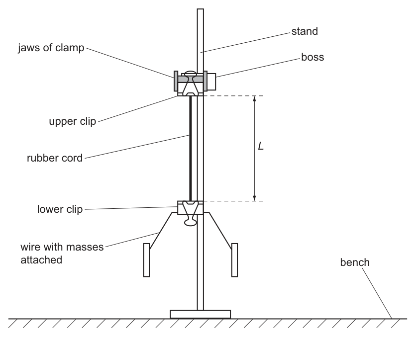
• The length of cord between the two clips is $L$ , as shown in Fig. 2.2.

Measure and record $L$ .

$L$ = ______

1M Similar

(iii)

• Keeping the cord vertical, rotate the lower clip through approximately $180^{\circ}$ and release the clip. The clip will rotate with a small number of oscillations.

• Take measurements to determine the period $T$ of these oscillations.

$T$ = ______ $\text{s}$

2M Similar

DifficultyMedium-Easy

Worked solution

Working

Time $N$ oscillations (e.g. $N = 10$ ) and divide by $N$ .

Example: for $N = 10$ , measured time $t = 12.6\ \text{s}$ .

T = \frac{t}{N} = \frac{12.6}{10} = 1.26\ \text{s}

Answer

T = 1.26\ \text{s}

Final answer

T = 1.26 s (example)

Detailed explanation

Background Concept

The period $T$ is the time for one complete oscillation. Human reaction time is a significant fraction of a single period, so the standard technique is to time several oscillations and divide:

T = \frac{t}{N}

where $t$ is the total time for $N$ oscillations.

Understanding the Question

After twisting the lower clip by about $180^{\circ}$ and releasing, the system performs a small number of torsional oscillations. You must take measurements to determine $T$ .

Approach

Choose a clear reference position (e.g. when the lower clip passes a particular orientation).
Time $N$ complete oscillations with a stopwatch, where $N$ is reasonably large (e.g. 10) to reduce fractional timing error.
Repeat the measurement and average.

Step-by-Step Reasoning

Twist the lower clip by about $180^{\circ}$ , release without pushing sideways.
Start timing as the clip passes the chosen reference orientation.
Count $N$ full oscillations (returning to the same orientation each time) and stop the stopwatch.
Calculate:

T = \frac{t}{N}

Example:

If $N = 10$ and $t = 12.6\ \text{s}$ ,

T = \frac{12.6}{10} = 1.26\ \text{s}

Repeat and take a mean $T$ .

Key Takeaways

Timing many cycles reduces the percentage effect of reaction time.
Using a consistent reference point improves repeatability.

Common Mistakes

Timing a single oscillation (large percentage uncertainty).
Miscounting oscillations (especially as amplitude decays).
Starting/stopping at different points in the oscillation.

Things to Be Careful About

The cord must remain vertical; sideways motion changes the oscillation and the period.
Use the same amplitude range each time (very large twists may change behaviour of rubber).

Techniques used

time multiple oscillations and divide to obtain the perioduse a consistent reference point for timingrepeat timing measurements and take a mean

(c)

Using the shorter length of rubber cord, repeat (b).

$d$ = ______

$L$ = ______

$T$ = ______ $\text{s}$

3M Similar

DifficultyMedium-Easy

Worked solution

Answer

Repeat the measurements using the shorter cord.

Example recorded values:

d = 2.48\ \text{mm}

L = 30.0\ \text{cm}

Time $N = 10$ oscillations, e.g. $t = 10.8\ \text{s}$ :

T = \frac{10.8}{10} = 1.08\ \text{s}

Final answer

d = 2.48 mm, L = 30.0 cm, T = 1.08 s (example)

Detailed explanation

Background Concept

To compare behaviour for different cord lengths, you must keep the method the same: same way of measuring $d$ and $L$ , same timing method for $T$ , and as many controlled conditions as possible (same masses, same twist angle, same reference point).

Understanding the Question

You now use the shorter rubber cord and repeat part (b), meaning you must again measure and record $d$ , $L$ and the oscillation period $T$ for this new cord.

Approach

Replace the longer cord with the shorter cord while keeping the rest of the apparatus unchanged.
Measure $d$ with a micrometer (repeat and average).
Measure $L$ between the two clips.
Determine $T$ by timing multiple oscillations and dividing.

Step-by-Step Reasoning

Measure diameter $d$ as before, taking care not to compress rubber.
Measure $L$ with the cord hanging vertically and stationary.
For the period, time $N$ oscillations (e.g. 10) and compute $T=t/N$ .
Example set of values:

d = 2.48\ \text{mm},\quad L = 30.0\ \text{cm},\quad T = 1.08\ \text{s}

Your numbers will depend on your own readings.

Key Takeaways

Consistency of method matters when comparing two sets of results.
Repetition (for both $d$ and timing) improves reliability.

Common Mistakes

Measuring a different definition of $L$ in the second run.
Forgetting to use the same number of oscillations $N$ for timing.
Failing to re-measure $d$ (diameter can differ between cords).

Things to Be Careful About

Ensure the shorter cord is still securely held and does not slip in the clips.
Keep the same masses and the same value of $B$ for both runs.

Techniques used

repeat the same measurement procedure for a second configurationmeasure diameter and length to appropriate precisiontime multiple oscillations and divide to obtain the period

(d)

It is suggested that the relationship between $T$ , $B$ , $L$ and $d$ is

T^2 = \frac{B^2 L}{kd^4}

where $k$ is a constant.

(i)

Using your data, calculate two values of $k$ .

first value of $k$ = ______

second value of $k$ = ______

1M Similar

DifficultyMedium

Worked solution

Working

From

T^2 = \frac{B^2 L}{kd^4}

k = \frac{B^2 L}{d^4 T^2}

Using example data (convert to SI):

$B = 8.20\ \text{cm} = 0.0820\ \text{m}$

Longer cord:

$L_1 = 45.0\ \text{cm} = 0.450\ \text{m}$ , $d_1 = 2.50\ \text{mm} = 2.50\times 10^{-3}\ \text{m}$ , $T_1 = 1.26\ \text{s}$

k_1 = \frac{(0.0820)^2(0.450)}{(2.50\times 10^{-3})^4(1.26)^2} = 4.88\times 10^{7}

Shorter cord:

$L_2 = 30.0\ \text{cm} = 0.300\ \text{m}$ , $d_2 = 2.48\ \text{mm} = 2.48\times 10^{-3}\ \text{m}$ , $T_2 = 1.08\ \text{s}$

k_2 = \frac{(0.0820)^2(0.300)}{(2.48\times 10^{-3})^4(1.08)^2} = 4.57\times 10^{7}

Answer

First value of $k$ (example): $4.88\times 10^{7}$

Second value of $k$ (example): $4.57\times 10^{7}$

Final answer

k1 = 4.88×10^7, k2 = 4.57×10^7 (examples)

Detailed explanation

Background Concept

When you are given an experimental relationship with a constant $k$ , you test it by rearranging the equation to calculate $k$ from measured quantities. If the model is correct, the calculated $k$ should be (approximately) the same for different runs.

Here:

T^2 = \frac{B^2 L}{kd^4}

Rearranging to make $k$ the subject gives:

k = \frac{B^2 L}{d^4 T^2}

This is the expression you use with each set of measurements.

Understanding the Question

You have two data sets: one using the longer cord and one using the shorter cord. Using your measured $B$ , $L$ , $d$ and $T$ for each run, calculate two values of $k$ .

Approach

Rearrange the given equation for $k$ .
Convert all measurements into SI units (m, s).
Substitute each run’s $L$ , $d$ , $T$ (with the same $B$ ) into the expression for $k$ .
Obtain two values $k_1$ and $k_2$ .

Step-by-Step Reasoning

Start with the relationship and rearrange:

T^2 = \frac{B^2 L}{kd^4} \Rightarrow kT^2 = \frac{B^2 L}{d^4} \Rightarrow k = \frac{B^2 L}{d^4 T^2}

Use SI units. This is crucial because powers like $d^4$ make unit mistakes extremely large.
Compute $k$ $k$ separately for each cord length:
- For run 1 use $(L_1, d_1, T_1)$ .
- For run 2 use $(L_2, d_2, T_2)$ .
The two values should be reasonably close if the relationship is valid within experimental uncertainty.

Key Takeaways

Always rearrange to isolate the constant you are testing.
Convert to SI and be especially careful with powers ( $B^2$ and $d^4$ ).

Common Mistakes

Using $d^2$ instead of $d^4$ .
Leaving $d$ in mm and $B, L$ in cm (leads to wrong powers of ten).
Forgetting to square $T$ .

Things to Be Careful About

Keep enough significant figures in intermediate calculations; round only at the end.
Since $d$ is raised to the 4th power, a small percentage uncertainty in $d$ produces a much larger percentage uncertainty in $k$ (approximately 4 times).

Techniques used

rearrange an equation to make a constant the subjectsubstitute measured values consistently in SI unitscalculate and compare two experimental values of a constant

(ii)

Justify the number of significant figures that you have given for your values of $k$ .

1M Similar

DifficultyMedium-Easy

Worked solution

Answer

$k$ is calculated from measured quantities and has a large uncertainty (notably from $d^4$ and timing), so quoting $k$ to 2 significant figures is appropriate (consistent with an uncertainty of order $\sim 20\%$ ).

Final answer

2 significant figures (justified by measurement uncertainty)

Detailed explanation

Background Concept

Significant figures in a calculated result should reflect the precision of the measurements used. A useful rule is: if the percentage uncertainty is a few percent, 3 s.f. may be reasonable; if it is large (e.g. $\sim 10\%$ to $20\%$ ), then 2 s.f. (or even 1 s.f.) is more appropriate.

For a product/power relationship, percentage uncertainties approximately add with powers:

\frac{\Delta k}{k} \approx 2\frac{\Delta B}{B} + \frac{\Delta L}{L} + 4\frac{\Delta d}{d} + 2\frac{\Delta T}{T}

So the $d^4$ term tends to dominate.

Understanding the Question

You must explain why you wrote your values of $k$ to a particular number of significant figures. The examiner wants to see that you have matched the rounding to the measurement uncertainty (or to the least precise measurement).

Approach

Identify which measured quantities have the largest percentage uncertainty.
Note that $d$ is raised to the 4th power, so its uncertainty greatly affects $k$ .
Conclude an appropriate s.f. for $k$ (commonly 2 s.f. for large uncertainties like $\sim 20\%$ ).

Step-by-Step Reasoning

Even if $d$ is measured to $\pm 0.01\ \text{mm}$ , the percentage uncertainty might be around:

\frac{0.01}{2.50}\times 100 \approx 0.4\%

But because $d$ is to the 4th power, this contributes roughly $4\times 0.4\% \approx 1.6\%$ to $k$ .
Timing uncertainties and judgement of centres/lengths can add further uncertainty; the question later suggests $20\%$ uncertainty in $k$ , which is large.
With $\sim 20\%$ uncertainty, giving $k$ to 2 s.f. is sensible (more digits would imply false precision).

Key Takeaways

Rounding is about uncertainty, not about how many digits your calculator shows.
Powers (like $d^4$ ) amplify uncertainty.

Common Mistakes

Quoting $k$ to 4 or 5 significant figures because the calculator gives them.
Quoting different significant figures for the two values without reason.

Things to Be Careful About

If your measurements are only to 2–3 s.f., it is rarely justified for a derived constant to be more precise than 2–3 s.f.
Use the question’s suggested $20\%$ as strong evidence that 2 s.f. is appropriate.

Techniques used

identify the least precise measured quantityjustify significant figures using percentage uncertaintyround a calculated constant appropriately

(e)

It is suggested that the percentage uncertainty in the values of $k$ is $20\%$ .

Using this uncertainty, explain whether your results support the relationship in (d).

1M Similar

DifficultyMedium-Easy

Worked solution

Working

Compare $k_1$ and $k_2$ using percentage difference (example):

\%\ \text{difference} = \frac{|k_1-k_2|}{\frac{1}{2}(k_1+k_2)}\times 100

With $k_1 = 4.88\times 10^{7}$ and $k_2 = 4.57\times 10^{7}$ ,

\%\ \text{difference} = \frac{0.31\times 10^{7}}{4.725\times 10^{7}}\times 100 = 6.6\%

Since $6.6\% < 20\%$ , the two values agree within uncertainty.

Answer

Yes, the results support the relationship because the two values of $k$ differ by less than $20\%$ (within the stated uncertainty).

Final answer

Supports the relationship (difference < 20%)

Detailed explanation

Background Concept

To decide whether results support a model, you check whether values that should be constant (here $k$ ) are consistent within experimental uncertainty. A simple consistency check is whether the percentage difference between two values is less than (or comparable to) the stated percentage uncertainty.

Understanding the Question

You are told to assume the percentage uncertainty in $k$ is $20\%$ . You calculated two values of $k$ (from long and short cord). You must state whether the agreement between these two values is good enough to support the suggested relationship.

Approach

Compute how different the two $k$ values are (percentage difference).
Compare this percentage difference with $20\%$ .
Conclude: if difference $\lesssim 20\%$ , results support the relationship; if much larger, they do not.

Step-by-Step Reasoning

A common method is:

\%\ \text{difference} = \frac{|k_1-k_2|}{\text{mean of }k_1\text{ and }k_2}\times 100

where mean $= \tfrac{1}{2}(k_1+k_2)$ .

If the percentage difference is smaller than $20\%$ , the discrepancy is explainable by the uncertainty, so the experiment is consistent with the model.
If larger than $20\%$ , the discrepancy is too large to be explained by uncertainty alone, so the model may not be supported (or there are systematic errors).

Key Takeaways

Agreement “within uncertainty” is the key phrase for Paper 3 conclusions.
Use the uncertainty threshold given, not an arbitrary judgement.

Common Mistakes

Comparing absolute difference $|k_1-k_2|$ without converting to a percentage.
Saying “supports” without any quantitative comparison.

Things to Be Careful About

Use the same basis for comparison (percentage difference compared to percentage uncertainty).
If your values are close to the threshold, phrase carefully: “consistent within the stated uncertainty”.

Techniques used

compare two experimental values using a percentage differencejudge agreement using an uncertainty thresholdstate a conclusion consistent with the comparison

(f)

(i)

Describe four sources of uncertainty or limitations of the procedure for this experiment.
For any uncertainties in measurement that you describe, you should state the quantity being measured and a reason for the uncertainty.

4M Similar

DifficultyMedium-Easy

Worked solution

Answer

Any four valid sources of uncertainty/limitations, e.g.

Timing $T$ with a stopwatch: reaction time when starting/stopping and difficulty deciding the exact reference position.
Counting oscillations: amplitude decays and motion may not be perfectly periodic, so it is easy to miscount cycles.
Measuring $B$ (centre-to-centre): centres are not sharply defined; alignment/parallax when reading the ruler.
Measuring $d$ : rubber compresses in the micrometer and the cord may not have uniform/circular cross-section (value of $d$ varies along the cord).

Final answer

See solution (four limitations listed)

Detailed explanation

Background Concept

Uncertainty and limitations in practical work come from:

instrument resolution (smallest scale division),
observer judgement (parallax, identifying reference points),
random variation (repeat readings scatter), and
systematic effects (consistent bias such as zero error, compression, slipping, non-ideal motion).

Good answers in Paper 3 are specific: name the quantity and give the physical reason.

Understanding the Question

You must describe four sources of uncertainty or limitations in this procedure. If you describe a measurement uncertainty, you must state which quantity (e.g. $B$ , $L$ , $d$ , $T$ ) and why it is uncertain.

Approach

Think through each measured quantity and the procedure:

$T$ : timed oscillations and counting.
$B$ : centre-to-centre distance using a ruler.
$L$ : distance between clips.
$d$ : micrometer measurement of a deformable, non-uniform cord.
Also consider procedural limitations: non-vertical cord, slipping in clips, damping, and twist angle not consistent.

Step-by-Step Reasoning

Four good, creditworthy examples (with quantity + reason):

$T$ (stopwatch reaction time)
- Starting and stopping the stopwatch depends on human reaction time.
- Also hard to judge the exact instant the lower clip passes a reference orientation.
$T$ (oscillations not perfectly steady)
- Motion is damped; amplitude decreases, which can make it difficult to decide when one full oscillation is completed.
- Small sideways motion can couple in, changing the apparent period.
$B$ (centre-to-centre distance)
- The “centre” of each slotted mass is not a sharp point; judgement is needed.
- Ruler may not be exactly aligned; parallax can occur.
$d$ (diameter measurement of rubber)
- Rubber compresses in the micrometer, causing a systematically smaller reading if too much force is used.
- Diameter may vary along the cord or the cord may be slightly oval.

Other acceptable limitations could include: measuring $L$ while the cord is still oscillating; $L$ changing slightly with time because rubber creeps; slipping at clips; twist not exactly $180^{\circ}$ each time.

Key Takeaways

Always link uncertainty to a specific measured quantity and a physical cause.
Damping and deformation are common limitations for rubber experiments.

Common Mistakes

Writing vague statements like “human error” with no quantity or reason.
Repeating the same idea in different words (only counts once).
Listing improvements instead of uncertainties (this part is limitations only).

Things to Be Careful About

Ensure you have four distinct points.
For measurement uncertainties, explicitly name the quantity ( $B$ , $L$ , $d$ , or $T$ ) to secure credit.

Techniques used

identify specific sources of random and systematic uncertaintylink each uncertainty to a measured quantitystate a physical reason for each limitation

(ii)

Describe four improvements that could be made to this experiment. You may suggest the use of other apparatus or different procedures.

4M Similar

DifficultyMedium

Worked solution

Answer

Any four valid improvements, e.g.

Improve timing: use video analysis / motion sensor / light gate with a marker on the clip to determine $T$ without reaction time.
Reduce timing uncertainty: time a larger number of oscillations (e.g. $20$ ) and repeat several times, then average.
Improve $d$ measurement: use a micrometer with ratchet and take readings at several positions/orientations; apply zero correction.
Improve geometry/alignment: use a fixed reference/pointer to define the reference orientation and ensure the cord is vertical (e.g. plumb line, rigid stand, minimise sideways motion).

Final answer

See solution (four improvements listed)

Detailed explanation

Background Concept

Improvements should directly reduce the uncertainties/limitations identified. The best responses pair an improvement with a specific problem (e.g. reaction time (\rightarrow) electronic timing).

Understanding the Question

You must describe four improvements. You may suggest different apparatus or procedures. The improvements should be realistic for a school laboratory and clearly improve the quality of the data.

Approach

Match improvements to common problems in this experiment:

Stopwatch/reaction time (\rightarrow) automated timing.
Small number of oscillations (\rightarrow) time more cycles and repeat.
Rubber deformation / varying diameter (\rightarrow) careful micrometer technique and averaging.
Poor alignment / inconsistent release (\rightarrow) better alignment and consistent reference point.

Step-by-Step Reasoning

Four strong improvements (with what they fix):

Use electronic timing (reduces reaction time in $T$ )
- Record the motion with a camera and determine $T$ from the video frames, or use a sensor/data logger if available.
Time more oscillations and repeat (reduces random timing uncertainty)
- Measure time for $N=20$ oscillations instead of a small number, repeat 3 times, and take a mean.
Better diameter measurement (reduces uncertainty in $d$ and systematic compression)
- Use the micrometer ratchet consistently; measure at several points along the cord and in different orientations; average; correct for zero error.
Improve consistency of oscillations (reduces systematic changes to period)
- Use a pointer and protractor to set the initial twist angle consistently (about $180^{\circ}$ each time).
- Ensure the cord is vertical and the masses are not swinging sideways; use a rigid stand and release carefully.

Other valid improvements include: marking clip positions to define $L$ clearly; shielding from drafts to reduce damping variability; ensuring clips do not slip (roughen/secure clamping surfaces).

Key Takeaways

Improvements must be specific and clearly linked to reduced uncertainty.
Better instruments and more repeats are the most common routes to better data.

Common Mistakes

Giving vague improvements like “be more careful”.
Repeating the same improvement (e.g. “repeat readings” in multiple forms).
Suggesting changes that do not address any identified limitation.

Things to Be Careful About

Provide four distinct improvements.
Make sure each suggested improvement is practical and clearly improves a measurement or the oscillation behaviour.

Techniques used

propose procedural changes that reduce specific uncertaintiessuggest improved instruments for more precise measurementsincrease repeatability by standardising the method