Physics 9702/31 — May/June 2025

Cambridge AS Level · Advanced Practical Skills · worked solutions for every part, with the mark scheme

questions

marks

120

minutes

Topics Manipulation, Measurement and Observation · Presentation of Data and Observations · Analysis, Conclusions and Evaluation

Q1MediumManipulation, Measurement and ObservationPresentation of Data and ObservationsAnalysis, Conclusions and Evaluation

In this experiment, you will investigate the oscillation of masses on springs.

You have been provided with masses and springs.

Set up the apparatus as shown in Fig. 1.1.

Fig. 1.1

(a)

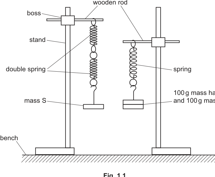
● Ensure the bottoms of both masses are at the same level.
● Pull both masses down through a short distance and release them at the same time.
● Watch the oscillations of the masses. The masses initially oscillate in phase, then out of phase and then back in phase.
● The number of oscillations of mass S from release until the masses are back in phase for the first time is $n_0$ .

Determine and record $n_0$ .

$n_0$ = ______

2M Similar

DifficultyMedium-Easy

Worked solution

Count the number of oscillations of mass $S$ from release until the two masses are back in phase for the first time; repeat and take a mean.

A typical recorded value is:

n_0 = 25.0

Final answer

n0 = 25.0

Detailed explanation

Background Concept

Two oscillators with slightly different periods will not stay in step. If they start in phase, the phase difference increases with time because one completes cycles slightly faster. They will become out of phase, and later return to being in phase again when the phase difference has increased by $2\pi$ (one extra cycle).

The key experimental skill here is recognising “in phase again” (same position and same direction of motion at the same instant) and counting the number of oscillations of mass $S$ until the first time that happens.

Understanding the Question

You set up two vertical mass–spring oscillators side-by-side and ensure the bottoms of the masses are level. You pull both down slightly and release at the same time.

You then observe:

they start in phase,
later become out of phase,
then come back in phase.

You must determine $n_0$ , defined as the number of oscillations made by mass $S$ from release until they are back in phase for the first time.

Approach

Make the initial conditions as similar as possible (small amplitude, simultaneous release, same starting position relative to equilibrium).
Decide on a consistent “counting point” for oscillations of $S$ (e.g. each time it passes equilibrium going upwards).
Watch for the first time both masses are again moving together (same direction) and at the same relative point in their motion.
Repeat to reduce random judgment error, then record a mean.

Step-by-Step Reasoning

Align the bottoms of the two masses: this is a practical reference that makes it easier to judge whether the two masses are together (in phase).
Displace both by a short distance and release simultaneously: small amplitude helps keep the period close to constant and makes motion easier to compare.
Start counting oscillations of mass $S$ using one consistent reference (e.g. count each full cycle as “down → up → down”).
Observe when the two masses first return to being in phase: they should pass the same positions at the same time and move in the same direction.
Stop the count at that first re-phasing, record $n_0$ .
Repeat the run and average; if two values disagree noticeably, repeat again and choose a consistent method of deciding the “back in phase” moment.

Key Takeaways

“Back in phase” means same part of cycle and same direction.
A clear counting rule + repeats improves reliability.

Common Mistakes

Counting half-oscillations inconsistently (sometimes peak-to-peak, sometimes equilibrium-to-equilibrium).
Stopping when they are at the same height but moving in opposite directions (that is out of phase).
Using a large amplitude (can make motion harder to compare and may introduce non-ideal effects).

Things to Be Careful About

Only the first time they return to in phase is $n_0$ .
Parallax: view at eye level with the masses.
Release timing: if releases are not simultaneous, judging phase becomes harder.

Techniques used

align the reference levels of two oscillating systemsrelease both oscillators simultaneously with a small amplitudecount oscillations until the first re-phasing eventrepeat observations and take a mean value

(b)

(i)

● Add a mass of $30\text{ g}$ to mass S. The added mass is $M$ .
● Record $M$ .

$M$ = ______

● Repeat (a). The number of oscillations of mass S from release until the masses are back in phase for the first time is $n$ .
● Determine and record $n$ .

$n$ = ______

1M Similar

DifficultyEasy

Worked solution

Added mass:

M = 30\ \text{g} = 0.030\ \text{kg}

Repeat the observation in (a) and record a typical value:

n = 20.6

Final answer

M = 0.030 kg, n = 20.6

Detailed explanation

Background Concept

For a mass–spring oscillator, changing the mass changes the period. Here, you are not asked to calculate the period; instead you observe how many oscillations occur before the two oscillators re-phase.

The experimental skill is keeping the method identical while changing only one variable (the added mass $M$ ).

Understanding the Question

You add $30\ \text{g}$ to mass $S$ (this added amount is defined as $M$ ). You must:

record $M$ ,
repeat the phase observation from (a) to obtain $n$ (oscillations of $S$ until first re-phasing).

Approach

Record $M$ clearly with a unit (preferably SI).
Repeat exactly the same release and counting method used for $n_0$ .

Step-by-Step Reasoning

Add the $30\ \text{g}$ mass securely to $S$ .
Record the added mass as $M = 30\ \text{g}$ (or $0.030\ \text{kg}$ ).
Ensure the bottoms are level again (the equilibrium position shifts when mass changes).
Displace and release both masses at the same time with a small amplitude.
Count oscillations of $S$ until the first time they are back in phase; record this as $n$ .

Key Takeaways

Change only $M$ ; keep the rest of the method the same.
Always include a unit when recording masses.

Common Mistakes

Recording the total mass on $S$ instead of the added mass $M$ .
Forgetting to re-level the masses after adding $M$ .

Things to Be Careful About

If you choose to use $\text{kg}$ , convert correctly: $30\ \text{g} = 0.030\ \text{kg}$ .
Use consistent precision for $n$ across different runs (e.g. same counting definition each time).

Techniques used

convert added masses into SI units for recordingrepeat the oscillation observation under changed massrecord measured quantities with unit and appropriate precision

(ii)

Calculate $N$ , where

N = n_0 - n

$N$ = ______

1M Similar

(c)

Vary $M$ by changing the number of $10\text{ g}$ masses added to mass S and determine $n$ . Do not use $M = 0$ .

Repeat until you have five sets of values of $M$ and $n$ .

Record your results in a table. Include values of $N$ . Also include values of $N^3$ to three significant figures.

8M Similar

DifficultyMedium

Worked solution

Record five sets of $M$ and $n$ (with $M \neq 0$ ), then calculate $N = n_0-n$ and $N^3$ (3 s.f.).

Example of a correctly presented table:

$M / \text{kg}$	$n$	$N = n_0-n$	$N^3$
0.020	21.09	3.91	59.8
0.030	20.60	4.40	85.2
0.040	20.19	4.81	111
0.050	19.87	5.13	135
0.060	19.57	5.43	160

Final answer

Table of M, n, N and N^3 (3 s.f.), with five non-zero M values.

Detailed explanation

Background Concept

In Paper 3, marks for tables usually depend on:

having enough readings (here five sets, and not using $M=0$ ),
choosing a sensible range of the independent variable ( $M$ ),
recording raw data consistently,
calculating derived quantities correctly (here $N$ and $N^3$ ),
presenting everything in one clear table with correct headings and units.

$N$ is defined by:

N = n_0 - n

and you must also calculate:

N^3

Understanding the Question

You must:

Change $M$ by adding different numbers of $10\ \text{g}$ masses to $S$ (so $M$ changes in steps of $0.010\ \text{kg}$ if you record in SI).
For each $M$ , repeat the observation to get $n$ .
For each run, calculate $N$ and then $N^3$ .
Put all values into a table, including $N^3$ to three significant figures.

Approach

Choose five different non-zero values of $M$ across a reasonable range.
For each $M$ , measure $n$ using the same method.
Use your previously measured $n_0$ (from part (a)) as the constant reference and compute $N$ .
Cube $N$ and round $N^3$ to 3 s.f.
Present in one table with headings containing quantity and unit (especially for $M$ ).

Step-by-Step Reasoning

Select $M$ values: e.g. $0.020\ \text{kg}$ to $0.060\ \text{kg}$ in steps of $0.010\ \text{kg}$ gives five readings and uses the provided $10\ \text{g}$ masses.
For each $M$ , repeat the release and counting procedure to obtain $n$ .
Calculate $N$ for each row:

N = n_0 - n

For example, if $n_0 = 25.00$ and $n = 20.60$ :

N = 25.00 - 20.60 = 4.40

Calculate $N^3$ and round to 3 s.f.:

N^3 = (4.40)^3 = 85.184 \approx 85.2

Table presentation:

Put all results in one table.
Include units in the heading for $M$ (e.g. $M/\text{kg}$ ).
Keep consistent decimal places within columns (e.g. $M$ to 3 d.p. if in kg, and $n$ to a consistent precision).

Key Takeaways

Five non-zero $M$ readings are required.
Derived columns ( $N$ , $N^3$ ) must be calculated correctly and presented clearly.
$N^3$ must be to 3 s.f..

Common Mistakes

Including $M=0$ (explicitly disallowed).
Mixing units (some $M$ in g, some in kg) or missing units in the heading.
Rounding $N$ too aggressively, then getting poor $N^3$ values.
Writing $N^3$ with too many/few significant figures.

Things to Be Careful About

Ensure $n_0$ used in all calculations is the same measured value from part (a).
If $n_0$ and $n$ are recorded to a certain precision, keep $N$ consistent with that.
When cubing, use sufficient calculator precision before rounding $N^3$ to 3 s.f.

Techniques used

vary the independent variable in suitable steps and obtain at least five readingsrecord results in a single table with correct headings and unitscalculate derived quantities from measurements including a powerapply consistent significant figures and decimal places within each column

(d)

(i)

Plot a graph of $N^3$ on the $y$ -axis against $M$ on the $x$ -axis.

3M Similar

(ii)

Draw the straight line of best fit.

1M Similar

(iii)

Determine the gradient and $y$ -intercept of this line.

gradient = ______
$y$ -intercept = ______

2M Similar

DifficultyMedium-Easy

Worked solution

Working

Using two points on the best-fit line, e.g.
$(M, N^3) = (0.020\ \text{kg}, 60)$ and $(0.060\ \text{kg}, 160)$ :

\text{gradient} = \frac{\Delta (N^3)}{\Delta M} = \frac{160-60}{0.060-0.020} = \frac{100}{0.040} = 2.50 \times 10^3

y\text{-intercept} = c = 60 - (2.50 \times 10^3)(0.020) = 10

Answer

gradient $= 2.50 \times 10^3\ \text{kg}^{-1}$

y-intercept $= 10$

Final answer

gradient = 2.50 × 10^3 kg^-1, y-intercept = 10

Detailed explanation

Background Concept

For a straight-line graph,

y = mx + c

$m$ is the gradient (slope):

m = \frac{\Delta y}{\Delta x}

$c$ is the y-intercept (value of $y$ when $x=0$ ).

On a plotted graph, you should use the best-fit line, not individual points, and choose two points far apart to reduce percentage reading error.

Understanding the Question

From your graph of $N^3$ (y-axis) against $M$ (x-axis), you must determine:

the gradient of the best-fit line,
the y-intercept of the best-fit line.

Approach

Draw a large right-angled triangle on the best-fit line.
Read two well-separated points from the best-fit line (not necessarily your data points).
Compute gradient using $\Delta (N^3) / \Delta M$ .
Find the y-intercept by extending the line to $M=0$ and reading $N^3$ , or by using $c = y - mx$ with a point on the line.

Step-by-Step Reasoning

diagram-1

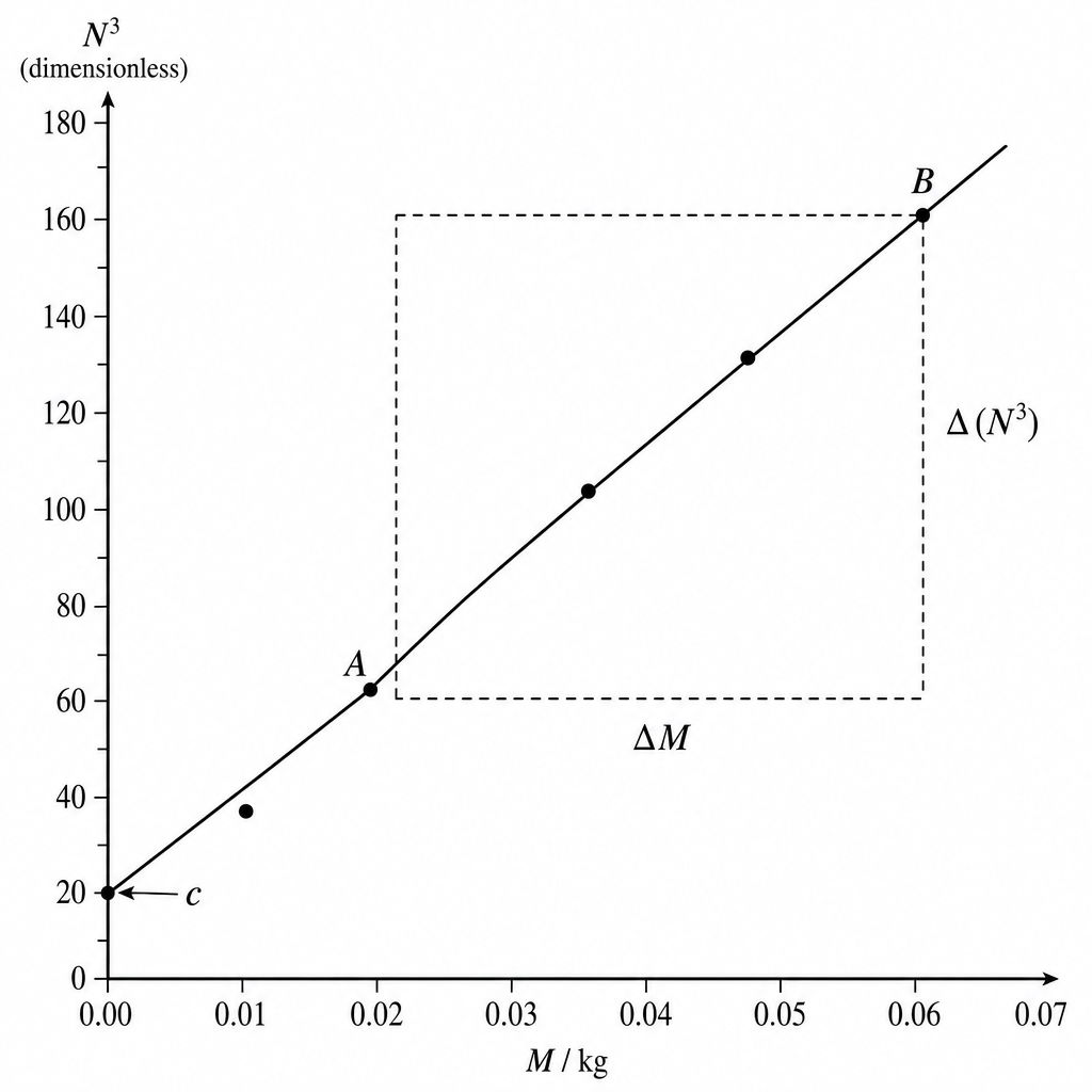
Choose two points on the best-fit line far apart (to make the triangle large). For example:

Point A: $M=0.020\ \text{kg}$ , $N^3=60$
Point B: $M=0.060\ \text{kg}$ , $N^3=160$

Calculate the gradient:

\Delta (N^3) = 160 - 60 = 100

\Delta M = 0.060 - 0.020 = 0.040\ \text{kg}

\text{gradient} = \frac{100}{0.040} = 2.50 \times 10^3\ \text{kg}^{-1}

The unit comes from $\text{(unit of }N^3) / \text{(unit of }M)$ , i.e. dimensionless per kg $= \text{kg}^{-1}$ .

Find the intercept using $c = y - mx$ with Point A:

c = 60 - (2.50\times 10^3)(0.020) = 60 - 50 = 10

This is the y-value when $M=0$ .

Key Takeaways

Use the best-fit line and a large triangle for gradient.
Gradient units come from $y/x$ .
Intercept can be read or calculated from $c=y-mx$ .

Common Mistakes

Using $x/y$ instead of $y/x$ .
Using two nearby points (large fractional uncertainty in gradient).
Calculating gradient from two experimental points that are not on the best-fit line.
Forgetting units for the gradient.

Things to Be Careful About

If you plotted $M$ in grams, the gradient unit would be $\text{g}^{-1}$ and the numerical value would change by a factor of $1000$ .
Read-off values should be consistent with your graph’s scale; do not overstate precision.

Techniques used

use a large triangle on the best-fit line to calculate gradientread two well-separated points from the best-fit linedetermine the y-intercept by extrapolation to the y-axis

(e)

It is suggested that the quantities $N$ and $M$ are related by the equation

N^3 = PM + Q

where $P$ and $Q$ are constants.

Using your answers in (d)(iii), determine the values of $P$ and $Q$ . Give appropriate units.

$P$ = ______
$Q$ = ______

2M Similar

DifficultyMedium-Easy

Worked solution

Given

N^3 = PM + Q

Comparing with $y = mx + c$ for a graph of $N^3$ (y-axis) against $M$ (x-axis):

P = \text{gradient} = 2.50 \times 10^3\ \text{kg}^{-1}

Q = y\text{-intercept} = 10

Final answer

P = 2.50 × 10^3 kg^-1, Q = 10

Detailed explanation

Background Concept

If you plot $y$ against $x$ and obtain a straight line, the equation is typically written as:

y = mx + c

gradient $m$ is the coefficient of $x$
intercept $c$ is the value of $y$ when $x=0$

Units:

If $y$ is dimensionless and $x$ has units of kg, then the gradient has units of $\text{kg}^{-1}$ .

Understanding the Question

You are told the suggested relationship is:

N^3 = PM + Q

You already found the gradient and y-intercept in (d)(iii) from the graph of $N^3$ against $M$ . You must use those to find $P$ and $Q$ and state appropriate units.

Approach

Map the suggested equation onto $y = mx + c$ $y = m x + c$ by identifying:
- $y \leftrightarrow N^3$
- $x \leftrightarrow M$
- $m \leftrightarrow P$
- $c \leftrightarrow Q$
Take $P$ from the gradient and $Q$ from the intercept.
Assign units from the axes.

Step-by-Step Reasoning

From the graph definition:

$y$ -axis is $N^3$ (dimensionless)
$x$ -axis is $M$ (e.g. in kg)

Compare

N^3 = PM + Q

y = mx + c

So:

P = m = \text{gradient}

Q = c = \text{y-intercept}

Using the representative values obtained:

P = 2.50 \times 10^3\ \text{kg}^{-1}

because $P$ has units $\text{(unit of }N^3) / \text{(unit of }M)$ , i.e.

\frac{1}{\text{kg}} = \text{kg}^{-1}.

And:

Q = 10

with no unit (dimensionless).

Key Takeaways

In a linear graph, gradient corresponds to the coefficient of $x$ and intercept to the constant term.
Units of gradient come from $y/x$ .

Common Mistakes

Swapping $P$ and $Q$ .
Giving $Q$ a unit (it is an intercept in $N^3$ , which is dimensionless).
Using the wrong mass unit (e.g. taking gradient from a kg graph but writing $\text{g}^{-1}$ ).

Things to Be Careful About

Your units for $P$ must match the unit you used for $M$ on the x-axis.
Quote $P$ and $Q$ to a sensible number of significant figures consistent with your graph readings.

Techniques used

identify the correspondence between a linear equation and a straight-line graphequate gradient and intercept to physical constantsdeduce the units of constants from the plotted variables

Q2MediumManipulation, Measurement and ObservationAnalysis, Conclusions and EvaluationPresentation of Data and Observations

In this experiment, you will investigate the behaviour of paper on water.

You have been provided with two sheets of tracing paper.

(a)

● On one of the sheets of tracing paper, draw two identical rectangles as shown in Fig. 2.1 where $c = 4.0\text{ cm}$ and $d = 6.0\text{ cm}$ . The orientation of the rectangles must be as shown in Fig. 2.1.
● Add labels A and B to the rectangles, as shown in Fig. 2.1.

Fig. 2.1

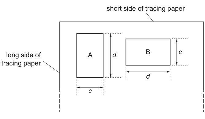
● Use the scissors to cut out the rectangles.
● Take measurements to determine the average value of $d$ .

$d$ = ______ $\text{cm}$

1M Similar

DifficultyMedium-Easy

Worked solution

Working

Measure $d$ for both cut rectangles (and/or at both ends of each rectangle) using a ruler with $1\ \text{mm}$ divisions.

Example readings: $6.0\ \text{cm}$ , $6.0\ \text{cm}$ , $6.0\ \text{cm}$ , $6.0\ \text{cm}$ .

Mean:

\overline{d} = \frac{6.0+6.0+6.0+6.0}{4} = 6.0\ \text{cm}

Answer

$d = 6.0\ \text{cm}$ (example, to $0.1\ \text{cm}$ )

Final answer

d = 6.0 cm

Detailed explanation

Background Concept

A length measurement should be recorded to the resolution of the instrument. With a typical ruler marked in $1\ \text{mm}$ , the resolution is $0.1\ \text{cm}$ . Repeating a measurement and taking a mean reduces the effect of random errors (small variations caused by judgement of edges, slight misalignment, etc.).

Understanding the Question

You draw two identical rectangles where the longer side is labelled $d = 6.0\ \text{cm}$ in the template. After cutting them out, you must measure $d$ and record an average value. The mark is for sensible measuring technique and a realistic recorded value/precision.

Approach

Use a ruler to measure the long side $d$ carefully (ruler aligned with edge, avoid parallax).
Take several readings (e.g. both rectangles, possibly both ends of each rectangle).
Calculate the mean and record to $0.1\ \text{cm}$ .

Step-by-Step Reasoning

Place the rectangle on the bench and align the ruler so the zero mark is at one end of the long edge.
Read the position of the far end of the long edge; read at eye level to avoid parallax.
Repeat for the second rectangle (and optionally repeat at a different point on the same edge to check straightness).
Add the readings and divide by the number of readings to obtain the mean $\overline{d}$ .
Record $\overline{d}$ in $\text{cm}$ to one decimal place if using a mm ruler.

Key Takeaways

Record lengths to the instrument resolution.
Repeats + mean improve reliability.
Keep units and consistent decimal places.

Common Mistakes

Recording $d$ with too many decimals (e.g. $6.000\ \text{cm}$ ) using a ruler.
Not taking repeats/mean when asked for an average.
Parallax error: reading the scale from an angle.

Things to Be Careful About

Ensure you measure the long side of the rectangle (that is $d$ ).
Start from the ruler’s zero mark (not the edge of the plastic) to reduce systematic offset.
Keep the same precision across all length readings you use in the mean.

Techniques used

measure a length using a ruler with appropriate precisiontake repeated readings and calculate a mean valuerecord a measured value with a consistent decimal place

(b)

(i)

● When A is placed flat on the surface of the water in one of the bowls, the shape will curl up as shown in Fig. 2.2. Two edges of the paper will curl and then meet.

Fig. 2.2

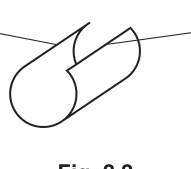
The time between placing A on the water and the two edges meeting is $T_A$ .

● Place A flat on the water.
● Determine $T_A$ .

$T_A$ = ______

● Remove A from the water and place it in the empty bowl.

2M Similar

DifficultyMedium-Easy

Worked solution

Working

Start timing when rectangle A first touches the water surface; stop timing when the two curling edges first meet.

Repeat and take a mean.

Example: $3.5\ \text{s}$ , $3.7\ \text{s}$ , $3.6\ \text{s}$

T_A = \frac{3.5+3.7+3.6}{3} = 3.6\ \text{s}

Answer

$T_A = 3.6\ \text{s}$ (example)

Final answer

T_A = 3.6 s

Detailed explanation

Background Concept

A time interval is measured by identifying a clear start event and a clear end event, then using a timing device (stopwatch). Repeating measurements and averaging reduces random timing scatter due to reaction time and judgement.

Understanding the Question

Rectangle A is placed flat on water. It curls until two edges meet. You must measure the time interval $T_A$ between (i) placing A on the water and (ii) the instant the two edges meet.

Approach

Decide precisely what counts as “start” and “end” for timing.
Use a stopwatch and repeat the measurement several times.
Compute a mean value for $T_A$ and record it to the appropriate precision (usually $0.1\ \text{s}$ if using a digital stopwatch).

Step-by-Step Reasoning

Hold A just above the water surface so you can release it smoothly and consistently.
Start the stopwatch at the instant the paper first contacts the water (or at release, but be consistent).
Watch the edges as they curl. Stop the stopwatch at the first moment the two edges touch.
Record the time.
Repeat at least 3 times (removing and drying/replacing the paper as required by the procedure) and calculate the mean:

T_A = \frac{\sum T}{n}

Quote $T_A$ with an appropriate number of decimal places.

Key Takeaways

Define the timed event clearly.
Repeats + mean improve reliability.
Consistent start/stop criteria matter more than “perfect” judgement.

Common Mistakes

Starting timing before the paper touches the water or after it has already begun curling (inconsistent start).
Stopping timing when edges are “close” rather than when they actually meet.
Only taking one timing (large random uncertainty).

Things to Be Careful About

Keep water conditions similar each time (still water, similar temperature).
Avoid touching the paper while it curls.
Record to the resolution of the stopwatch (often $0.1\ \text{s}$ ).

Techniques used

use a stopwatch to measure a time intervaldefine a clear start and end point for timingrepeat a timing measurement and calculate a mean

(ii)

Estimate the percentage uncertainty in your value of $T_A$ . Show your working.

percentage uncertainty = ______ $\%$

1M Similar

DifficultyMedium-Easy

Worked solution

Working

Take absolute uncertainty in $T_A$ as half the range of repeats.

Example repeats: $3.5\ \text{s}$ to $3.7\ \text{s}$

\Delta T_A = \frac{3.7-3.5}{2} = 0.10\ \text{s}

Percentage uncertainty:

\%\ \text{uncertainty} = \frac{\Delta T_A}{T_A}\times 100 = \frac{0.10}{3.6}\times 100 = 2.8\% \approx 3\%

Answer

percentage uncertainty $\approx 3\%$ (example)

Final answer

Detailed explanation

Background Concept

Uncertainty in a measured time can be estimated in two common ways:

From repeats (random uncertainty): take half the range, (\Delta T = (T_\text{max}-T_\text{min})/2).
From instrument/reaction time: for hand timing, reaction time often dominates (commonly around $0.2\ \text{s}$ for start/stop combined), but the repeat-range method is often accepted if you have several readings.

Percentage uncertainty is

\%\ \text{uncertainty} = \frac{\Delta T}{T} \times 100.

Understanding the Question

You must estimate the percentage uncertainty in your measured $T_A$ and show working. The method must link to how you measured $T_A$ (e.g. repeats, or stopwatch reaction time).

Approach

Choose a justified absolute uncertainty $\Delta T_A$ (half-range is a good standard method if you repeated readings).
Divide by the mean value $T_A$ .
Multiply by 100 and round sensibly.

Step-by-Step Reasoning

Using three repeats is typical. If your times vary between $3.5\ \text{s}$ and $3.7\ \text{s}$ , that spread reflects random variability. Half the spread is taken as the uncertainty in the mean time:

\Delta T_A = \frac{3.7-3.5}{2} = 0.10\ \text{s}.

Then convert to percentage:

\frac{0.10}{3.6} = 0.0278 \Rightarrow 2.78\% \approx 3\%.

Key Takeaways

Percentage uncertainty compares uncertainty size to the measurement itself.
Repeats allow you to estimate random uncertainty using half-range.

Common Mistakes

Using full range instead of half-range.
Forgetting to multiply by 100.
Using a $\Delta T$ much smaller than the stopwatch resolution or your reaction time without justification.

Things to Be Careful About

If you only took one reading, you must use a different estimate (e.g. reaction time); half-range cannot be used with one value.
Keep consistent significant figures: uncertainty typically 1 s.f. (or 2 s.f. if needed), percentage uncertainty usually to 1 s.f. or nearest whole percent.

Techniques used

estimate an absolute uncertainty from repeated readings or reaction timecalculate a percentage uncertainty using uncertainty divided by measured valueround an uncertainty to a sensible number of significant figures

(c)

(i)

● Repeat the procedure in (b)(i) for B. The time between placing B on the water and the two edges meeting is $T_B$ .

$T_B$ = ______

● Remove B from the water.
● Compare your values of $T_A$ and $T_B$ . Record the longer time.

longer time = ______

1M Similar

(ii)

The quantity $W$ is given by

W = \frac{\text{longer time}}{\text{shorter time}}

Calculate $W$ .

$W$ = ______

1M Similar

(iii)

Justify the number of significant figures that you have given for your value of $W$ .

1M Similar

DifficultyMedium-Easy

Worked solution

Answer

$W$ is found by dividing two measured times. $T_A$ and $T_B$ are recorded to $0.1\ \text{s}$ (about $2\ \text{s.f.}$ ), so $W$ should be given to $2\ \text{s.f.}$ (limited by the least precise time).

Final answer

W to 2 significant figures, limited by T_A and T_B

Detailed explanation

Background Concept

Significant figures communicate the precision of a value. For multiplication/division, the usual rule is:

The result should have the same number of significant figures as the input quantity with the fewest significant figures.

This prevents you from claiming an unrealistically precise derived value.

Understanding the Question

You calculated $W$ from

W = \frac{\text{longer time}}{\text{shorter time}}.

You must justify how many significant figures to use when writing $W$ .

Approach

Look at how precisely you measured the times (e.g. to nearest $0.1\ \text{s}$ ).
Identify which of the two times has fewer significant figures.
Quote $W$ to that number of significant figures.

Step-by-Step Reasoning

If your times are recorded as, for example, $3.6\ \text{s}$ and $2.4\ \text{s}$ :

Each is to the nearest $0.1\ \text{s}$ and each has $2\ \text{s.f.}$ .
Therefore $W$ should be to $2\ \text{s.f.}$ .

Even if your calculator gives $1.5000...$ , that extra precision is not justified because the times themselves are not known that precisely.

Key Takeaways

Derived values must not be more precise than the measurements used.
For ratios, match s.f. to the least precise measured input.

Common Mistakes

Giving $W$ to 3 or 4 s.f. just because the calculator shows it.
Confusing decimal places with significant figures.

Things to Be Careful About

If one time was recorded to fewer s.f. than the other (e.g. $3.6\ \text{s}$ and $2\ \text{s}$ ), then $W$ must follow the smaller s.f. count.
Justification must explicitly refer to the precision/s.f. of $T_A$ and $T_B$ .

Techniques used

identify the limiting measurement in a calculationapply significant-figure rules for divisionjustify rounding based on measurement precision

(d)

Repeat (a), (b)(i), (c)(i) and (c)(ii) using new rectangles with $c = 4.0\text{ cm}$ and $d = 9.0\text{ cm}$ .

$d$ = ______ $\text{cm}$
$T_A$ = ______
$T_B$ = ______
longer time = ______
$W$ = ______

3M Similar

DifficultyMedium-Easy

Worked solution

Working

Make new rectangles with $c = 4.0\ \text{cm}$ and $d = 9.0\ \text{cm}$ . Measure $d$ (mean) and determine $T_A$ , $T_B$ as before.

Example measurements:

$d = 9.0\ \text{cm}$
$T_A = 5.5\ \text{s}$
$T_B = 3.0\ \text{s}$
longer time $= 5.5\ \text{s}$ , shorter time $= 3.0\ \text{s}$

W = \frac{5.5}{3.0} = 1.83

Answer

$d = 9.0\ \text{cm}$ (example)

$T_A = 5.5\ \text{s}$ (example)

$T_B = 3.0\ \text{s}$ (example)

longer time $= 5.5\ \text{s}$ (example)

$W = 1.8$ (example, $2\ \text{s.f.}$ )

Final answer

Example: d = 9.0 cm, T_A = 5.5 s, T_B = 3.0 s, longer time = 5.5 s, W = 1.8

Detailed explanation

Background Concept

To test a suggested relationship, you need results for at least two different values of the variable (here $d$ ). You must repeat the same method so that any change in results is due to changing $d$ , not changing the procedure.

Understanding the Question

You repeat the earlier steps but now with rectangles of long side $d = 9.0\ \text{cm}$ . You must measure $d$ , measure $T_A$ and $T_B$ , decide which is longer, and calculate

W = \frac{\text{longer time}}{\text{shorter time}}.

Approach

Make the new rectangles carefully so only $d$ changes.
Measure $d$ with repeats and take a mean.
Time $T_A$ and $T_B$ using the same start/stop definition.
Compute $W$ and record to appropriate s.f.

Step-by-Step Reasoning

Construct rectangles with the required dimensions and orientation.
Measure $d$ several times and calculate an average.
Time curling for A and for B; repeat and average each time if possible.
Identify the larger time as the “longer time”.
Divide longer by shorter to get $W$ (no units).

Key Takeaways

Change one variable ( $d$ ) while keeping the method consistent.
Record measurements with consistent precision.

Common Mistakes

Forgetting to maintain the orientation of rectangles A and B.
Calculating $W$ using a fixed order (e.g. always $T_A/T_B$ ) rather than longer/shorter.

Things to Be Careful About

With a larger $d$ , the curling behaviour may be slower or more uneven; define the “meeting” point consistently.
Keep water conditions similar to earlier trials so the comparison across $d$ is meaningful.

Techniques used

repeat an experimental procedure for a different value of the independent variablemeasure lengths and times to consistent precisioncalculate a ratio from measured values

(e)

It is suggested that the relationship between $W$ and $d$ is

W^2 = kd

where $k$ is a constant.

Using your data, calculate two values of $k$ .

first value of $k$ = ______
second value of $k$ = ______

1M Similar

DifficultyMedium-Easy

Worked solution

Working

From

W^2 = kd

k = \frac{W^2}{d}

Using example data for $d=6.0\ \text{cm}$ , $W=1.50$ :

k_1 = \frac{(1.50)^2}{6.0} = \frac{2.25}{6.0} = 0.375

Using example data for $d=9.0\ \text{cm}$ , $W=1.83$ :

k_2 = \frac{(1.83)^2}{9.0} = \frac{3.35}{9.0} = 0.372

Answer

first value of $k = 0.375$ (example)

second value of $k = 0.372$ (example)

Final answer

Example: k1 = 0.375, k2 = 0.372

Detailed explanation

Background Concept

If a relationship has the form

W^2 = kd,

then for each experimental pair $(W,d)$ you can compute

k = \frac{W^2}{d}.

If the suggested relationship is correct and conditions are controlled, $k$ should be approximately constant (same for different $d$ ).

Understanding the Question

You have two sets of data (one for $d\approx 6.0\ \text{cm}$ and one for $d\approx 9.0\ \text{cm}$ ). You must calculate two values of $k$ , one from each data set.

Approach

Rearrange to make $k$ the subject.
For each data set: square $W$ , divide by $d$ .
Quote the two values of $k$ .

Step-by-Step Reasoning

Rearrangement:

W^2 = kd \Rightarrow k = \frac{W^2}{d}.

Substitute your first $(W,d)$ pair to get $k_1$ .
Substitute your second $(W,d)$ pair to get $k_2$ .
Compare them informally: they should be close if the model is supported.

Key Takeaways

Use the model equation to calculate an implied constant.
Consistency of the constant across trials is evidence supporting the model.

Common Mistakes

Using $k = W/d$ instead of $W^2/d$ .
Forgetting to square $W$ .
Mixing up which $W$ belongs to which $d$ .

Things to Be Careful About

$W$ is dimensionless; $d$ is a length, so $k$ has units of $1/\text{length}$ if you track units (but the question does not require units here).
Keep sufficient s.f. in intermediate steps; round at the end.

Techniques used

rearrange an equation to make the constant the subjectsubstitute experimental values into an expressioncalculate and compare two values of a constant

(f)

It is suggested that the percentage uncertainty in the values of $k$ is $20\%$ .

Using this uncertainty, explain whether your results support the relationship in (e).

1M Similar

DifficultyMedium

Worked solution

Working

With $20\%$ uncertainty, each $k$ value has an allowed range of $\pm 20\%$ .

Example: $k_1 = 0.375$ gives range:

0.375\pm 0.20\times 0.375 = 0.375\pm 0.075

i.e. $0.300$ to $0.450$ .

$k_2 = 0.372$ lies within this range, so the two values agree within $20\%$ .

Answer

Yes. The two values of $k$ are consistent within $20\%$ , so the results support $W^2 = kd$ (within experimental uncertainty).

Final answer

Supports the relationship within 20% uncertainty

Detailed explanation

Background Concept

Experimental results never match a model perfectly because of uncertainties. A common way to test consistency is to check whether two values agree within a stated percentage uncertainty.

If a quantity $k$ has percentage uncertainty $p\%$ , then an acceptable interval is

k \pm \left(\frac{p}{100}\right)k.

If the intervals overlap (or one value lies inside the other’s interval), the results are consistent.

Understanding the Question

You calculated two values $k_1$ and $k_2$ from two data sets. You are told the percentage uncertainty in $k$ is $20\%$ . You must decide whether the difference between $k_1$ and $k_2$ is small enough that the model is supported.

Approach

Apply $\pm 20\%$ to one (or both) values to form an acceptable range.
Check if the other value falls within that range (or equivalently check overlap).
State a conclusion explicitly: supports / does not support.

Step-by-Step Reasoning

Using example values $k_1 = 0.375$ and $k_2 = 0.372$ :

Compute $20\%$ of $k_1$ :

0.20\times 0.375 = 0.075.

So acceptable range for $k_1$ is

0.375 \pm 0.075 \Rightarrow 0.300 \text{ to } 0.450.

Since $0.372$ lies in $0.300$ to $0.450$ , the two values agree within the stated uncertainty.

An alternative check is percentage difference:

\frac{|k_1-k_2|}{\text{mean}}\times 100

and see if it is $\le 20\%$ .

Key Takeaways

Agreement “within uncertainty” is the correct criterion, not exact equality.
Turning a percentage uncertainty into a numerical range makes comparison easy.

Common Mistakes

Saying “supports” just because the values are close, without referencing the $20\%$ .
Comparing using absolute difference only, without considering the scale of the values.

Things to Be Careful About

Make sure you use $20\%$ of the value (multiply by $0.20$ ), not add/subtract $20$ .
If your two $k$ values differ by more than $20\%$ , you should say the results do not support the relationship (at that uncertainty level).

Techniques used

apply a percentage uncertainty to create an acceptable rangecompare two values considering their uncertainty rangesconclude whether results are consistent with a suggested relationship

(g)

(i)

Describe four sources of uncertainty or limitations of the procedure for this experiment.

For any uncertainties in measurement that you describe, you should state the quantity being measured and a reason for the uncertainty.

4M Similar

DifficultyMedium

Worked solution

Answer

Timing uncertainty in $T_A$ and $T_B$ : stopwatch reaction time and judgement of the instant the edges first meet.
Inconsistent start condition: paper may not be placed equally flat / may contact water at slightly different times across its area, changing when curling begins.
Water surface conditions not controlled: surface contamination/soap/grease or ripples change wetting/surface tension and hence curling rate.
Rectangles not identical: cutting/drawing inaccuracies mean $d$ (and edge quality) varies; rough/uneven edges wet differently, affecting curling and the time to meet.

Final answer

Four limitations listed (timing, start condition, water surface, rectangle accuracy)

Detailed explanation

Background Concept

In practical experiments, uncertainties come from:

Measurement uncertainty (instrument resolution, reaction time, judgement of events).
Random errors (uncontrolled variations between repeats).
Systematic errors (consistent bias, e.g. miscalibrated ruler).
Limitations (features of the method that restrict accuracy or validity, e.g. poorly defined end-point).

Good exam answers name the quantity affected and give a clear physical reason.

Understanding the Question

You must describe four sources of uncertainty or limitations in the procedure. For measurement uncertainties, you must explicitly state what quantity is uncertain and why.

Approach

Pick four distinct issues from different parts of the method:

timing ( $T_A$ , $T_B$ )
defining the start/end events
controlling conditions (water surface/temperature)
making consistent paper samples (dimensions/edges)

For each one: “Quantity: … ; Reason: …”.

Step-by-Step Reasoning

Possible high-credit limitations include:

$T_A$ and $T_B$ (time) uncertainty: human reaction time starting/stopping the stopwatch introduces random scatter; the exact instant of “edges meet” is hard to judge.
Start condition variability: if the paper is dropped from slightly different heights/angles, or traps air, the initial wetting differs, changing the curling behaviour.
Water surface condition: ripples from previous trials, bowl vibrations, or nearby movement can move the paper; contamination changes surface tension so curling rate changes.
Dimensions/edge quality: small differences in $d$ or rough edges lead to different wetting and stiffness along the edge; this changes curling dynamics.

Other acceptable limitations (if distinct) could include: temperature changes during the experiment, paper becoming saturated between repeats, bowl edge effects if the curling paper touches the bowl, or asymmetrical curling (edges do not meet uniformly).

Key Takeaways

State the quantity and the reason.
Use specific, experimental causes rather than vague “human error”.

Common Mistakes

Writing generic statements like “parallax error” without saying what was being read.
Listing four points that are really the same issue (e.g. reaction time repeated in different words).
Giving improvements instead of limitations (this part is uncertainties/limitations only).

Things to Be Careful About

Ensure each point is distinct and clearly explained.
Link to the actual procedure: cutting paper, placing on water, timing edge meeting.
Avoid claiming unrealistic precision in timing when the endpoint is subjective.

Techniques used

identify sources of random and systematic uncertaintylink each uncertainty to a specific measured quantitystate a physical reason for each limitation

(ii)

Describe four improvements that could be made to this experiment. You may suggest the use of other apparatus or different procedures.

4M Similar

DifficultyMedium

Worked solution

Answer

Repeat timings and average $T_A$ and $T_B$ for each rectangle to reduce random error; discard anomalies.
Video the motion (phone camera) and determine the frame when edges first meet to reduce reaction-time/end-point uncertainty.
Use a template and sharp cutter (or printed rectangles) to make rectangles with more accurate/consistent $d$ and smoother edges.
Control water conditions: use clean water, allow water to settle between trials, and keep temperature constant (e.g. same room, measure temperature) to reduce variation in surface tension/wetting.

Final answer

Four improvements listed (repeats, video timing, better cutting/template, control water conditions)

Detailed explanation

Background Concept

Improvements should be directly linked to reducing either:

uncertainty in measured quantities (time/length),
variability in initial conditions,
uncontrolled environmental variables,
or limitations in how well the model can be tested.

A strong improvement is specific and explains how it reduces the stated limitation.

Understanding the Question

You need four improvements (apparatus or procedure changes). These should clearly address the uncertainties/limitations from part (g)(i).

Approach

For each limitation, propose a practical fix:

reaction time -> video/data logging
random variation -> repeats/averaging
inconsistent sample geometry -> template/cutter
uncontrolled water surface -> clean/settle/temperature control

Step-by-Step Reasoning

Repeats and mean: Taking 3–5 timings for each condition and averaging reduces random scatter and makes $W$ (and hence $k$ ) more reliable.
Video analysis: Recording the curling and stepping through frames gives a clearer definition of the instant of edge meeting; it greatly reduces human reaction time uncertainty.
Improve sample consistency: Using a printed template, set square, and a sharp craft knife on a cutting mat (rather than freehand scissors) improves the accuracy of $d$ and makes edges smoother and more uniform.
Control water conditions: Use fresh clean water, avoid detergent/grease, wait for ripples to stop, and keep temperature constant; all of these reduce variation in surface tension and wetting, which affect curling.

Other valid improvements could include using a larger bowl to avoid edge effects, using a consistent release method (e.g. a simple frame to lower the paper onto the surface), or using multiple different values of $d$ (more than two) to test the relationship more convincingly.

Key Takeaways

Improvements must be specific and linked to a limitation.
Better control + better measurement precision = more reliable test of a relationship.

Common Mistakes

Repeating the same idea four times (e.g. “take more readings” phrased differently).
Suggesting unrealistic equipment (e.g. light gates) that cannot detect “edges meeting”.
Giving improvements that do not address the main uncertainty (timing/end-point definition).

Things to Be Careful About

Make sure your improvements are feasible for the described experiment.
State how each improvement reduces uncertainty or variability, not just what to do.
If you propose more $d$ values, you should also mention how you would analyse (e.g. graph of $W^2$ against $d$ for a straight line).

Techniques used

propose procedural improvements that reduce uncertaintymatch each improvement to a corresponding limitationsuggest apparatus changes to improve measurement precision