Physics 9702/35 — October/November 2024

Cambridge AS Level · Advanced Practical Skills · worked solutions for every part, with the mark scheme

questions

marks

120

minutes

Topics Manipulation, Measurement and Observation · Presentation of Data and Observations · Analysis, Conclusions and Evaluation

Q120MMediumManipulation, Measurement and ObservationPresentation of Data and ObservationsAnalysis, Conclusions and Evaluation

In this experiment, you will investigate the balancing of a metre rule.

(a)

• Set up the apparatus as shown in Fig. 1.1.

Fig. 1.1

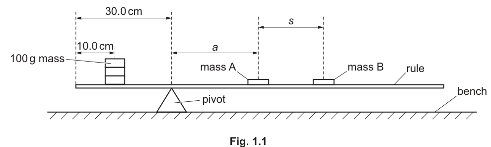
• Use the adhesive putty to fix three $100\text{ g}$ slotted masses with their centres above the $10.0\text{ cm}$ mark on the rule, as shown in Fig. 1.1.
• Place the rule on the pivot at the $30.0\text{ cm}$ mark.

The $100\text{ g}$ masses and the pivot must remain at these positions throughout the experiment.

• Place masses A and B on the rule.
• The distance between the centre of A and the pivot is $a$ .
The distance between the centre of B and the centre of A is $s$ .
Adjust the position of A until $a$ is approximately $20\text{ cm}$ .
• Adjust the position of B until the rule is balanced.
• Determine $a$ and $s$ .

$a$ = ______ $\text{cm}$
$s$ = ______ $\text{cm}$

1M Similar

DifficultyMedium-Easy

Worked solution

Answer

When the rule is balanced, measure the centre positions $x_A$ and $x_B$ on the rule.

a = x_A - 30.0\ \text{cm}

s = x_B - x_A\ \text{cm}

Example set of readings (to $0.1\ \text{cm}$ ):

$a = 20.0\ \text{cm}$

$s = 40.0\ \text{cm}$

Final answer

Student-dependent (e.g. a = 20.0 cm, s = 40.0 cm)

Detailed explanation

Background Concept

A metre rule balances about a pivot when the net moment (turning effect) about the pivot is zero. The moment of a force about a pivot is

\text{moment} = F \times \text{perpendicular distance from pivot}

For vertical weights acting on a horizontal rule, the perpendicular distance is simply the horizontal distance along the rule. Balance occurs when clockwise moments equal anticlockwise moments.

Understanding the Question

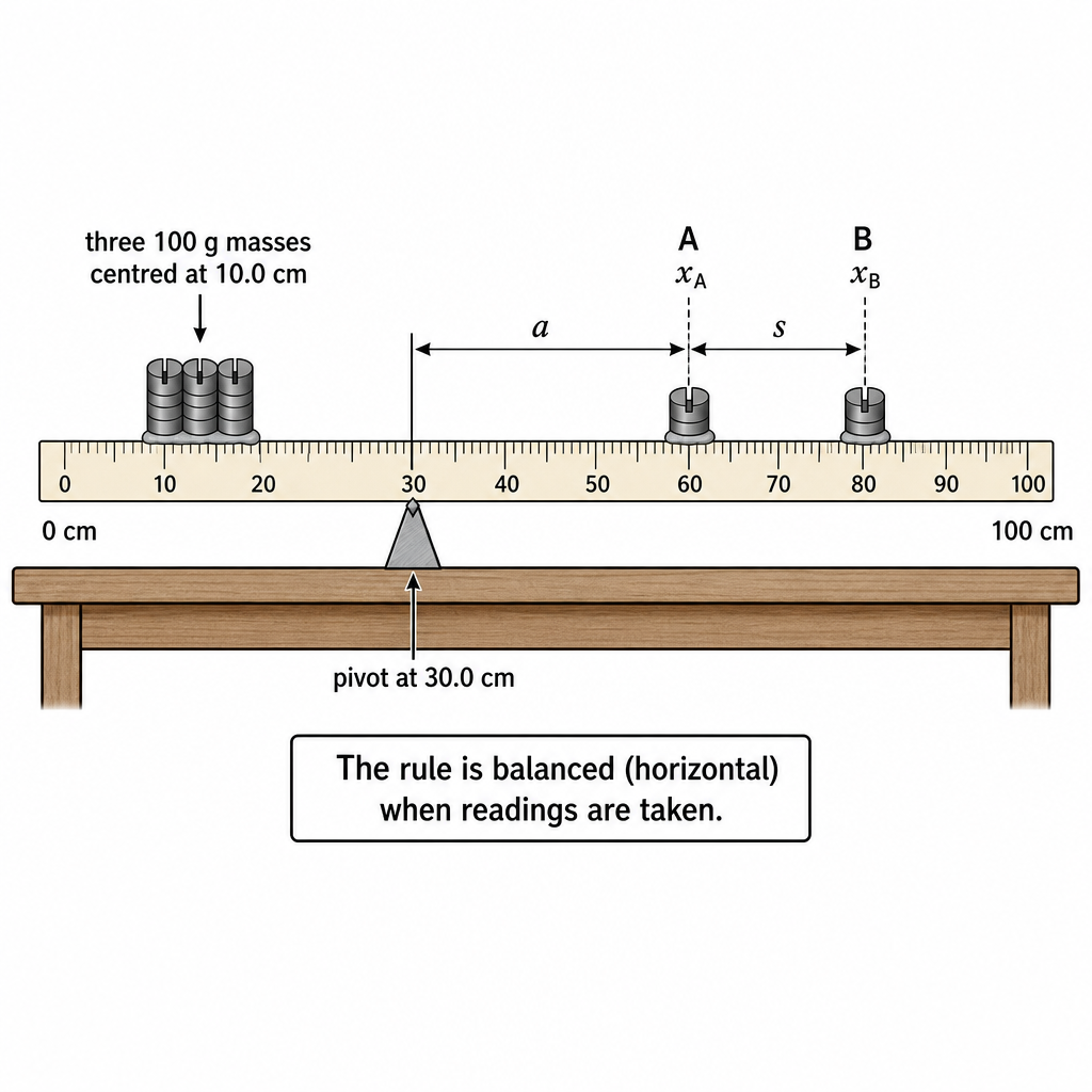
You are given a fixed arrangement: three $100\ \text{g}$ masses at the $10.0\ \text{cm}$ mark and a pivot at the $30.0\ \text{cm}$ mark (these must not move). You then place two other masses, A and B, to the right side and:

adjust A so that its distance from the pivot, $a$ , is about $20\ \text{cm}$
adjust B until the rule is balanced
measure $a$ (pivot to A) and $s$ (A to B).

The key is that $a$ and $s$ are not direct scale readings; they are distances between centres, found by subtracting scale positions.

diagram-1a

Approach

Balance the rule by sliding B until the rule is horizontal and not rotating.
Read the scale positions of the centres of A and B, call them $x_A$ and $x_B$ .
Convert these to the requested distances using subtraction:
- $a = x_A - 30.0$
- $s = x_B - x_A$
Record $a$ and $s$ to the precision of the rule (typically to $0.1\ \text{cm}$ ).

Step-by-Step Reasoning

Ensure the pivot is exactly at $30.0\ \text{cm}$ and the three $100\ \text{g}$ masses are fixed with their centres above $10.0\ \text{cm}$ .
Place A to the right of the pivot and move it until the distance from pivot to the centre of A is about $20\ \text{cm}$ .
Place B to the right and slide it until the rule balances (stays horizontal with no tendency to rotate).
Read the centre positions on the rule:
- Example: if $x_A = 50.0\ \text{cm}$ , then

a = 50.0 - 30.0 = 20.0\ \text{cm}

Example: if $x_B = 90.0\ \text{cm}$ , then

s = 90.0 - 50.0 = 40.0\ \text{cm}

Record the values clearly with units.

Key Takeaways

Distances $a$ and $s$ are found by subtracting scale readings.
Balance means zero net moment about the pivot.
Quote measurements to appropriate precision and include units.

Common Mistakes

Measuring $a$ from the end of the rule instead of from the pivot at $30.0\ \text{cm}$ .
Using the edge of a slotted mass instead of the centre of the mass.
Recording too many/few decimal places (e.g. $20.03\ \text{cm}$ from a ruler, or $20\ \text{cm}$ when $0.1\ \text{cm}$ is possible).
Not waiting for the rule to settle before taking readings.

Things to Be Careful About

Avoid parallax when reading the scale; view directly above the mark.
Ensure the pivot point is a single contact (knife-edge/edge) so the balance point is well-defined.
Keep the fixed masses and the pivot at the specified marks throughout, as required by the instructions.

Techniques used

set up the balancing apparatus as shown and keep fixed components unchangedadjust a sliding mass until a target distance is obtainedbalance the rule by moving a second mass until no rotation occursread positions on a metre rule and calculate distances by subtraction

(b)

Change the position of A. Adjust the position of B until the rule is balanced. Determine $a$ and $s$ .
Repeat until you have six sets of values of $a$ and $s$ . Do not use values of $a$ less than $10.0\text{ cm}$ .

Record your results in a table. Include values of $\frac{1}{a}$ and $\frac{s}{a}$ in your table.

10M Similar

DifficultyMedium

Worked solution

Answer

Obtain six different balanced positions with $a \ge 10.0\ \text{cm}$ . For each balance, record $a$ and $s$ (to $0.1\ \text{cm}$ ), then calculate $\dfrac{1}{a}$ and $\dfrac{s}{a}$ .

Record all results in one table with headings and units:

$a / \text{cm}$	$s / \text{cm}$	$\left(\dfrac{1}{a}\right) / \text{cm}^{-1}$	$\left(\dfrac{s}{a}\right)$
10.0	60.0	0.100	6.00
14.0	52.0	0.0714	3.71
18.0	44.0	0.0556	2.44
22.0	36.0	0.0455	1.64
26.0	28.0	0.0385	1.08
30.0	20.0	0.0333	0.667

Final answer

Student-dependent (six sets of a, s with calculated 1/a and s/a)

Detailed explanation

Background Concept

In practical work, you often need:

a sufficiently large number of readings to identify a trend (here, six pairs of $a$ and $s$ )
a suitable range of the independent variable (here, $a$ must be varied and must not be below $10.0\ \text{cm}$ )
a clear table with correct headings (quantity and unit) and consistent significant figures.

Derived quantities like $\dfrac{1}{a}$ and $\dfrac{s}{a}$ are calculated from measured values. Their precision should reflect the precision of the measured data.

Understanding the Question

You must change the position of A to create different values of $a$ , then each time move B until the rule is balanced and measure the corresponding $s$ .

You then need a results table containing four columns: $a$ , $s$ , $1/a$ , and $s/a$ . The instruction "Do not use values of $a$ less than $10.0\ \text{cm}$ " means you should choose A positions that keep $a$ at or above this limit.

Approach

Choose a series of A positions giving different $a$ values (at least 6), all $\ge 10.0\ \text{cm}$ .
For each $a$ , adjust B until balance, then measure $s$ .
Immediately calculate the two derived columns:

\frac{1}{a}

and

\frac{s}{a}

Present all results in one table with clear headings; keep decimal places consistent within each column.

Step-by-Step Reasoning

Start with one balanced configuration and measure $a$ and $s$ .
Move A to change $a$ $a$ (e.g. increase it by several cm each time). Each time:
- re-balance by sliding B
- read $x_A$ and $x_B$ and calculate $a$ and $s$ by subtraction
- record $a$ and $s$ to $0.1\ \text{cm}$ .
Calculate derived values:
- Example for $a = 22.0\ \text{cm}$ :

\frac{1}{a} = \frac{1}{22.0} = 0.0455\ \text{cm}^{-1}

Example for $s = 36.0\ \text{cm}$ and $a = 22.0\ \text{cm}$ :

\frac{s}{a} = \frac{36.0}{22.0} = 1.64

Put all six sets into a single table. Ensure the derived quantities are quoted to a sensible number of significant figures (commonly 3 s.f. for calculated values).

Key Takeaways

Collect enough data points (six) and a good range of $a$ to make a reliable graph.
Always include units in table headings (not in every cell).
Derived columns should be calculated consistently and presented clearly.

Common Mistakes

Using fewer than six readings.
Allowing $a < 10.0\ \text{cm}$ .
Missing units in headings or writing units inside the body of the table.
Inconsistent precision (e.g. mixing $0.1\ \text{cm}$ and $0.01\ \text{cm}$ in the same column without justification).
Calculating $1/a$ using $a$ in metres but labelling as $\text{cm}^{-1}$ (unit mismatch).

Things to Be Careful About

Keep the pivot and the three fixed $100\ \text{g}$ masses at the stated positions throughout.
Make sure the rule is truly balanced before reading: small oscillations should die away.
Check that B stays on the rule (does not hang off the end) as you change $a$ ; choose your $a$ range accordingly.

Techniques used

systematically vary the position of one mass while keeping other conditions constantre-balance the system for each setting and record paired measurementscalculate derived quantities from raw measurements with correct significant figurespresent results in a single table with clear headings and units

(c)

(i)

Plot a graph of $\frac{s}{a}$ on the $y$ -axis against $\frac{1}{a}$ on the $x$ -axis.

3M Similar

DifficultyMedium

Worked solution

Answer

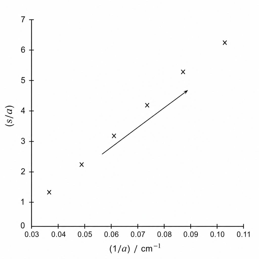
Plot $y = \dfrac{s}{a}$ (no unit) on the $y$ -axis against $x = \dfrac{1}{a}$ (units $\text{cm}^{-1}$ ) on the $x$ -axis.

Use a sensible scale (at least half the graph paper in each direction).
Label axes: $\left(\dfrac{1}{a}\right) / \text{cm}^{-1}$ and $\left(\dfrac{s}{a}\right)$ .
Plot all six points accurately.

Final answer

Graph of s/a (y) against 1/a (x) plotted

Detailed explanation

Background Concept

A graph is used to reveal and test a relationship between variables. When you are told explicitly what to plot, marks are typically for:

correct variables on correct axes
correct axis labels with units
sensible scales (not cramped, not awkward)
accurate plotting.

Here, both plotted quantities are derived from measurements: $1/a$ and $s/a$ .

Understanding the Question

You have a results table containing values of $a$ and $s$ , and the calculated values of $1/a$ and $s/a$ . You must plot:

vertical axis: $\dfrac{s}{a}$
horizontal axis: $\dfrac{1}{a}$ .

Because $a$ is measured in cm, $1/a$ has units $\text{cm}^{-1}$ . The ratio $s/a$ is dimensionless.

diagram-1ci

Approach

Decide which column in your table is $x$ and which is $y$ .
Choose axis limits that include all points with some margins.
Use an easy-to-read scale (e.g. 1 big square = 0.01 or 0.02 $\text{cm}^{-1}$ on the x-axis, depending on your range).
Plot each data point as a small cross.

Step-by-Step Reasoning

From your table, take each pair $\left(\dfrac{1}{a},\dfrac{s}{a}\right)$ .
Mark the axes:
- x-axis label: $\left(\dfrac{1}{a}\right) / \text{cm}^{-1}$
- y-axis label: $\left(\dfrac{s}{a}\right)$
Choose a scale that spreads the points well. For example, if $1/a$ ranges from about $0.033\ \text{cm}^{-1}$ to $0.100\ \text{cm}^{-1}$ , you might choose x-axis from $0.03$ to $0.11$ .
Plot all six points carefully (do not join dot-to-dot).

Key Takeaways

Always include units on axes (except for dimensionless quantities).
A good scale and accurate plotting are essential for reliable gradient/intercept values later.

Common Mistakes

Swapping axes (plotting $1/a$ on y and $s/a$ on x).
Missing units on the x-axis label.
Using a scale that uses only a small portion of the grid.
Plotting points as large blobs (reduces accuracy for best-fit line).

Things to Be Careful About

If $a$ is in cm in your table, keep $1/a$ in $\text{cm}^{-1}$ (do not switch to metres partway through).
Check each plotted point corresponds to the correct row (mixing rows is a common practical error).

Techniques used

select graph axes consistent with the required variableslabel axes with quantity and unitchoose a scale that uses a large fraction of the gridplot data points accurately as small crosses

(ii)

Draw the straight line of best fit.

1M Similar

DifficultyMedium-Easy

Worked solution

Answer

Draw one straight line of best fit through the plotted points (using a ruler), with approximately equal scatter of points above and below the line.

Final answer

Straight line of best fit drawn

Detailed explanation

Background Concept

Experimental points rarely lie perfectly on a straight line due to random uncertainties. A best-fit line represents the overall trend and is used to determine gradient and intercept more reliably than using individual points.

Understanding the Question

You have already plotted $\dfrac{s}{a}$ against $\dfrac{1}{a}$ . You must now draw the straight line that best represents the trend of your points.

Approach

Use a ruler to draw a single straight line.
Place it so that the points are roughly evenly distributed above and below the line.
The line should go through the general cluster, not necessarily through the origin or through every point.

Step-by-Step Reasoning

Visually assess the overall trend of the points.
Position your ruler so that the line passes through the middle of the scatter.
Check you have not simply joined the first and last points unless they genuinely represent the trend.
Draw the line cleanly and extend it enough to read a reliable intercept.

Key Takeaways

A best-fit line is about the trend, not perfect point-to-point matching.
A well-drawn line improves the accuracy of gradient and intercept.

Common Mistakes

Joining points dot-to-dot.
Forcing the line through the origin without evidence.
Drawing a line that passes through an outlier and misses most other points.

Things to Be Careful About

If one point is clearly an outlier, do not force the line to pass through it; instead balance the fit across the other points.
Extend the line across the full plotted range to help read the y-intercept accurately.

Techniques used

use a ruler to draw a single straight line of best fitbalance the line so that points are distributed evenly about itignore minor scatter without forcing the line through all points

(iii)

Determine the gradient and $y$ -intercept of this line.

gradient = ______
$y$ -intercept = ______

2M Similar

DifficultyMedium

Worked solution

Working

Choose two well-separated points on the best-fit line, for example:

(x_1,y_1) = (0.100,\ 6.00),\quad (x_2,y_2) = (0.0333,\ 0.667)

\text{gradient} = \frac{\Delta y}{\Delta x} = \frac{6.00 - 0.667}{0.100 - 0.0333} = 80.0\ \text{cm}

From the best-fit line, at $x=0$ :

y\text{-intercept} = -2.00

Answer

gradient $= 80.0\ \text{cm}$

$y$ -intercept $= -2.00$

Final answer

gradient = 80.0 cm, y-intercept = -2.00

Detailed explanation

Background Concept

For a straight-line graph of the form

y = mx + c

the gradient is

m = \frac{\Delta y}{\Delta x}

the y-intercept is the value of $y$ when $x=0$ , i.e. $c$ .

Units: $m$ has units of (units of $y$ ) divided by (units of $x$ ). Here, $y = s/a$ is dimensionless and $x = 1/a$ has units $\text{cm}^{-1}$ , so the gradient has units $\text{cm}$ .

Understanding the Question

You have drawn a best-fit straight line on a graph of $\dfrac{s}{a}$ (y-axis) against $\dfrac{1}{a}$ (x-axis). You must find:

the gradient of the line
the y-intercept.

These are then used in part (d) to determine constants.

Approach

Pick two points on the drawn best-fit line, far apart, and read their coordinates accurately.
Compute the gradient using $\Delta y / \Delta x$ .
Extend the line to cut the y-axis and read the intercept at $x=0$ .
Quote gradient with correct units and sensible significant figures.

Step-by-Step Reasoning

Using points far apart reduces percentage uncertainty in $\Delta x$ and $\Delta y$ .
Suppose you read two points on the line:

(x_1,y_1)\ \text{and}\ (x_2,y_2)

Then:

\Delta y = y_1 - y_2,\quad \Delta x = x_1 - x_2

and:

m = \frac{\Delta y}{\Delta x}

Check units: since $x$ is in $\text{cm}^{-1}$ , dividing by $\text{cm}^{-1}$ gives cm.
For the intercept, go to $x=0$ on the axis and read where your line crosses the y-axis; that value is $c$ .

Key Takeaways

Always use points on the best-fit line, not necessarily raw plotted points.
Use a large triangle (far apart points) for accuracy.
The intercept is read at $x=0$ .

Common Mistakes

Calculating gradient as $\Delta x/\Delta y$ instead of $\Delta y/\Delta x$ .
Using two adjacent points (small triangle), giving a very uncertain gradient.
Forgetting units for the gradient.
Reading the intercept from the nearest data point rather than from the line at $x=0$ .

Things to Be Careful About

Keep consistent rounding: do not over-round intermediate coordinate readings.
Extend the best-fit line neatly to the y-axis; do not guess the intercept without extending the line.

Techniques used

construct a large triangle on the best-fit linecalculate gradient using change in y divided by change in xread the y-intercept from the extrapolated best-fit lineassign correct units to gradient and intercept

(d)

(i)

It is suggested that the quantities $a$ and $s$ are related by the equation

\frac{s}{a} = \frac{P}{a} + Q

where $P$ and $Q$ are constants.

Using your answers in (c)(iii), determine the values of $P$ and $Q$ .
Give appropriate units.

$P$ = ______
$Q$ = ______

2M Similar

DifficultyMedium-Easy

Worked solution

Working

Given

\frac{s}{a} = \frac{P}{a} + Q

Let

y = \frac{s}{a},\quad x = \frac{1}{a}

y = Px + Q

Hence:

$P$ = gradient
$Q$ = y-intercept

Using (c)(iii):

P = 80.0\ \text{cm}

Q = -2.00

Answer

$P = 80.0\ \text{cm}$

$Q = -2.00$ (no unit)

Final answer

P = 80.0 cm, Q = -2.00

Detailed explanation

Background Concept

If a relationship can be written in the straight-line form

y = mx + c

then plotting $y$ against $x$ gives:

gradient $m$
intercept $c$ .

Comparing an experimental equation to this form is the standard way to extract constants.

Understanding the Question

You are told the suggested relationship is

\frac{s}{a} = \frac{P}{a} + Q

and your graph is $\dfrac{s}{a}$ against $\dfrac{1}{a}$ . That means the graph has been chosen specifically to match the form $y = mx + c$ .

You must use your gradient and intercept from (c)(iii) to determine numerical values of $P$ and $Q$ , including appropriate units.

Approach

Identify what plays the role of $x$ and $y$ .
Rewrite the given equation to match $y = mx + c$ .
Read off $P$ and $Q$ from gradient and intercept.
Determine units:
- since $y$ is dimensionless and $x$ has units $\text{cm}^{-1}$ , the gradient must have units cm.

Step-by-Step Reasoning

Let

y = \frac{s}{a}

and

x = \frac{1}{a}

Then the suggested equation becomes

y = P x + Q

So:

$P$ corresponds to the gradient of the $y$ vs $x$ graph.
$Q$ corresponds to the y-intercept.

Unit check:

$y$ has no unit.
$x$ has unit $\text{cm}^{-1}$ .
So $P$ must have unit cm so that $Px$ is dimensionless.
$Q$ is added to a dimensionless quantity, so $Q$ is dimensionless.

Key Takeaways

Plot selection is designed to linearise the relationship.
Constants are obtained by comparing directly to $y=mx+c$ .
Units come from dimensional consistency.

Common Mistakes

Stating $P$ has units $\text{cm}^{-1}$ (it is the gradient, not the x-axis variable).
Giving a unit for $Q$ (it is dimensionless).
Using raw $a$ and $s$ values instead of using gradient/intercept from the graph.

Things to Be Careful About

Use your best-fit line values (not a single data point) for gradient/intercept.
Quote $P$ and $Q$ to a sensible number of significant figures consistent with your graph reading accuracy.

Techniques used

compare the experimental straight-line graph to y = mx + cidentify constants from gradient and interceptdeduce units from dimensional consistency

(ii)

Theory suggests that

P = \frac{(Z - R)d}{m}

where $Z = 300\text{ g}$ , $d = 20.0\text{ cm}$ , $m = 50\text{ g}$ and $R$ is a constant.

Using your value of $P$ , determine a value for $R$ .
Give an appropriate unit.

$R$ = ______

1M Similar

DifficultyMedium-Easy

Worked solution

Working

P = \frac{(Z - R)d}{m}

Rearrange:

R = Z - \frac{mP}{d}

Substitute $Z = 300\ \text{g}$ , $d = 20.0\ \text{cm}$ , $m = 50\ \text{g}$ , $P = 80.0\ \text{cm}$ :

R = 300 - \frac{50 \times 80.0}{20.0} = 300 - 200 = 100\ \text{g}

Answer

$R = 100\ \text{g}$

Final answer

R = 100 g

Detailed explanation

Background Concept

Often a practical gives you an experimental constant (here $P$ from the graph) and then asks you to use a theoretical model to calculate another parameter (here $R$ ).

You must rearrange algebra carefully and keep units consistent.

Understanding the Question

You are given:

P = \frac{(Z - R)d}{m}

with known values $Z = 300\ \text{g}$ , $d = 20.0\ \text{cm}$ , $m = 50\ \text{g}$ , and you use your measured/graph value of $P$ to find $R$ .

$Z$ and $R$ are both masses (in g), so $R$ will be in g.

Approach

Rearrange the equation to make $R$ the subject.
Substitute the known numerical values.
Check that units are consistent: $P$ and $d$ are in cm so that $\dfrac{P}{d}$ is dimensionless.

Step-by-Step Reasoning

Starting from:

P = \frac{(Z - R)d}{m}

Multiply both sides by $m$ :

mP = (Z - R)d

Divide by $d$ :

\frac{mP}{d} = Z - R

Rearrange:

R = Z - \frac{mP}{d}

Now substitute values (using your own $P$ from the graph):

R = 300 - \frac{50 \times 80.0}{20.0} = 100\ \text{g}

Key Takeaways

Rearrangement first, substitution second.
Keep consistent units (cm with cm; g with g).
The final unit for $R$ is grams.

Common Mistakes

Rearrangement error giving $R = Z + \dfrac{mP}{d}$ .
Mixing cm and m for $P$ and $d$ .
Forgetting to state the unit for $R$ .

Things to Be Careful About

Use your experimentally determined $P$ (from your graph) rather than a theoretical or assumed value.
Check the sign: if $P$ is positive, then $\dfrac{mP}{d}$ is positive, so $R$ should be less than $Z$ for this model.

Techniques used

rearrange an equation to make the required variable the subjectsubstitute experimental constant into a theoretical expressioncheck and state the unit of the calculated quantity

Q220MMediumManipulation, Measurement and ObservationPresentation of Data and ObservationsAnalysis, Conclusions and Evaluation

In this experiment, you will investigate the oscillations of a wooden rod.

(a)

(i)

You are provided with two identical wooden rods. The length of one rod is $L$ and the diameter of the rod is $d$ , as shown in Fig. 2.1.

Fig. 2.1

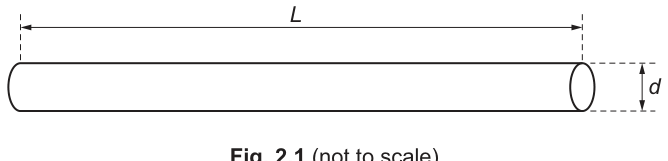
• Measure and record $L$ .

$L$ = ______

• Using the micrometer, measure and record $d$ .

$d$ = ______

• The volume $V$ of the rod is given by

V = \frac{\pi d^2 L}{4}

Calculate $V$ .

$V$ = ______

2M Similar

DifficultyMedium-Easy

Worked solution

Working

(Example readings)

$L = 0.600\ \text{m}$

$d = 0.02000\ \text{m}$

V = \frac{\pi d^2 L}{4}

V = \frac{\pi (0.02000)^2(0.600)}{4} = 1.885\times 10^{-4}\ \text{m}^3

Answer

$L = 0.600\ \text{m}$ , $d = 0.02000\ \text{m}$ , $V = 1.89\times 10^{-4}\ \text{m}^3$

Final answer

V = 1.89 × 10^-4 m^3

Detailed explanation

Background Concept

A wooden rod in this question is a cylinder. The volume of a cylinder is

V = A L

where $A$ is the cross-sectional area and $L$ is the length.

For a circular cross-section of diameter $d$ , the radius is $r = d/2$ , so

A = \pi r^2 = \pi \left(\frac{d}{2}\right)^2 = \frac{\pi d^2}{4}

Hence

V = \frac{\pi d^2 L}{4}

Understanding the Question

You must:

measure the rod length $L$ (using a rule),
measure the rod diameter $d$ (using a micrometer),
calculate the volume $V$ using the given formula.

Your exact values depend on your own measurements; what matters for marks is correct use of instruments, sensible recording, and correct calculation.

Approach

Measure $L$ carefully (read at eye level to reduce parallax).
Measure $d$ using a micrometer (check/allow for any zero error; gently close using the ratchet).
Convert to consistent units (best is SI: metres).
Substitute into $V = \pi d^2 L /4$ and calculate.

Step-by-Step Reasoning

Suppose you measure $L = 0.600\ \text{m}$ .
Suppose you measure $d = 0.02000\ \text{m}$ (e.g. $20.00\ \text{mm}$ ).
Substitute:

V = \frac{\pi (0.02000)^2(0.600)}{4}

Square the diameter:

(0.02000)^2 = 4.000\times 10^{-4}

Multiply by $L$ and divide by $4$ , then multiply by $\pi$ :

V = 1.885\times 10^{-4}\ \text{m}^3

Round to an appropriate number of significant figures (justified in part (a)(ii)).

Key Takeaways

Use the micrometer correctly (ratchet, zero error) for $d$ .
Keep units consistent before substituting.
A small fractional error in $d$ produces about double the fractional error in $V$ because $V \propto d^2$ .

Common Mistakes

Using $V = \pi d L$ or forgetting the $/4$ .
Mixing units (e.g. $d$ in mm and $L$ in m) without conversion.
Recording $d$ to too few decimal places for a micrometer (loses precision).
Not squaring $d$ .

Things to Be Careful About

Micrometer readings: include the main scale and thimble scale, and correct for zero error if present.
Measure $d$ at several positions along the rod and/or in two perpendicular directions if the rod is not perfectly circular; use a mean value (often improves reliability).

Techniques used

measure length with a rule while avoiding parallaxmeasure diameter with a micrometer and apply zero correctionsubstitute measured values into the cylinder volume formulaconvert all quantities into consistent SI units

(ii)

Justify the number of significant figures that you have given for your value of $V$ .

1M Similar

DifficultyMedium-Easy

Worked solution

Answer

$V$ is calculated using multiplication/division, so it should be given to the same number of significant figures as the least precise of $L$ and $d$ .

(For example, if $L$ is to $3\ \text{s.f.}$ and $d$ to $4\ \text{s.f.}$ , then $V$ should be to $3\ \text{s.f.}$ .)

Final answer

V to the same s.f. as the least precise of L and d (e.g. 3 s.f.).

Detailed explanation

Background Concept

Significant figures (s.f.) indicate the precision of a measured or calculated value. For a result obtained by multiplication/division, the standard rule is:

the answer should have the same number of significant figures as the quantity in the calculation that has the fewest significant figures.

This is because the least precise measurement limits the precision of anything calculated from it.

Understanding the Question

You have calculated $V$ from

V = \frac{\pi d^2 L}{4}

The question asks you to justify how many significant figures you wrote for $V$ .

Approach

Look at your recorded $L$ and $d$ .
Identify which one has fewer significant figures.
State that $V$ should be rounded to that number of significant figures.

Step-by-Step Reasoning

Suppose your measurements were like $L = 0.600\ \text{m}$ (3 s.f.) and $d = 0.02000\ \text{m}$ (4 s.f.).
Even though $d$ is very precise, the overall result cannot be more precise than the least precise measurement, here $L$ .
Therefore $V$ should be given to 3 s.f.

Also note: because $V \propto d^2$ , any percentage uncertainty in $d$ contributes twice to the percentage uncertainty in $V$ . This affects uncertainty analysis, but the significant-figure rule in the exam is usually still based on the least s.f. input.

Key Takeaways

For products/quotients, match the result’s s.f. to the least s.f. input.
Do not overstate precision in calculated quantities.

Common Mistakes

Giving $V$ to the same decimal places as $L$ .
Giving too many s.f. because a calculator shows many digits.
Ignoring that one measurement is clearly less precise.

Things to Be Careful About

Significant figures are not the same as decimal places.
If $L$ is recorded in cm and then converted to m, the s.f. do not change; only the power of ten changes.

Techniques used

identify the least significant-figure measurementstate that the calculated quantity should match the limiting precisionapply significant-figure rules for multiplication and division

(b)

(i)

• Set up the apparatus as shown in Fig. 2.2.

Fig. 2.2

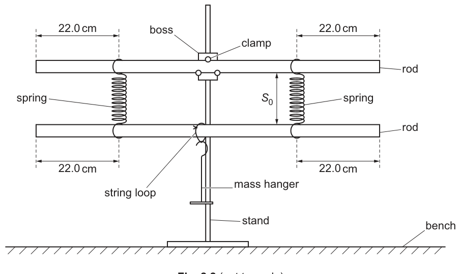
• Clamp one rod at its midpoint so that it is parallel to the bench.
• Slide the string loop onto the other rod.
• Slide the springs onto the rods and adjust the positions of the springs so that each spring is $22.0\text{ cm}$ from the nearest end of the rod, as shown in Fig. 2.2.
• Hang the mass hanger from the string loop. Adjust the position of the string loop so that it is at the midpoint of the lower rod.
• The distance between the two rods is $S_0$ .

Measure and record $S_0$ .

$S_0$ = ______ $\text{m}$

1M Similar

DifficultyMedium-Easy

Worked solution

Answer

(Example reading)

$S_0 = 0.120\ \text{m}$

Final answer

S0 = 0.120 m

Detailed explanation

Background Concept

In this experiment the separation $S$ between the two rods changes when extra weight is added, stretching the springs. Accurate measurements of $S_0$ and later $S_1$ are essential because the spring extension is found from a difference $(S_1 - S_0)$ .

Understanding the Question

You must set up the apparatus exactly as described (springs positioned $22.0\ \text{cm}$ from the ends, rods aligned, string loop at midpoint) and then measure the initial distance between rods, $S_0$ , in metres.

Approach

Ensure the rods are parallel and the lower rod is at rest.
Measure the vertical distance between corresponding points on the two rods (e.g. between their centres) using a ruler/metre rule held vertically.
Read the scale at eye level to reduce parallax.

Step-by-Step Reasoning

diagram-b-i-1

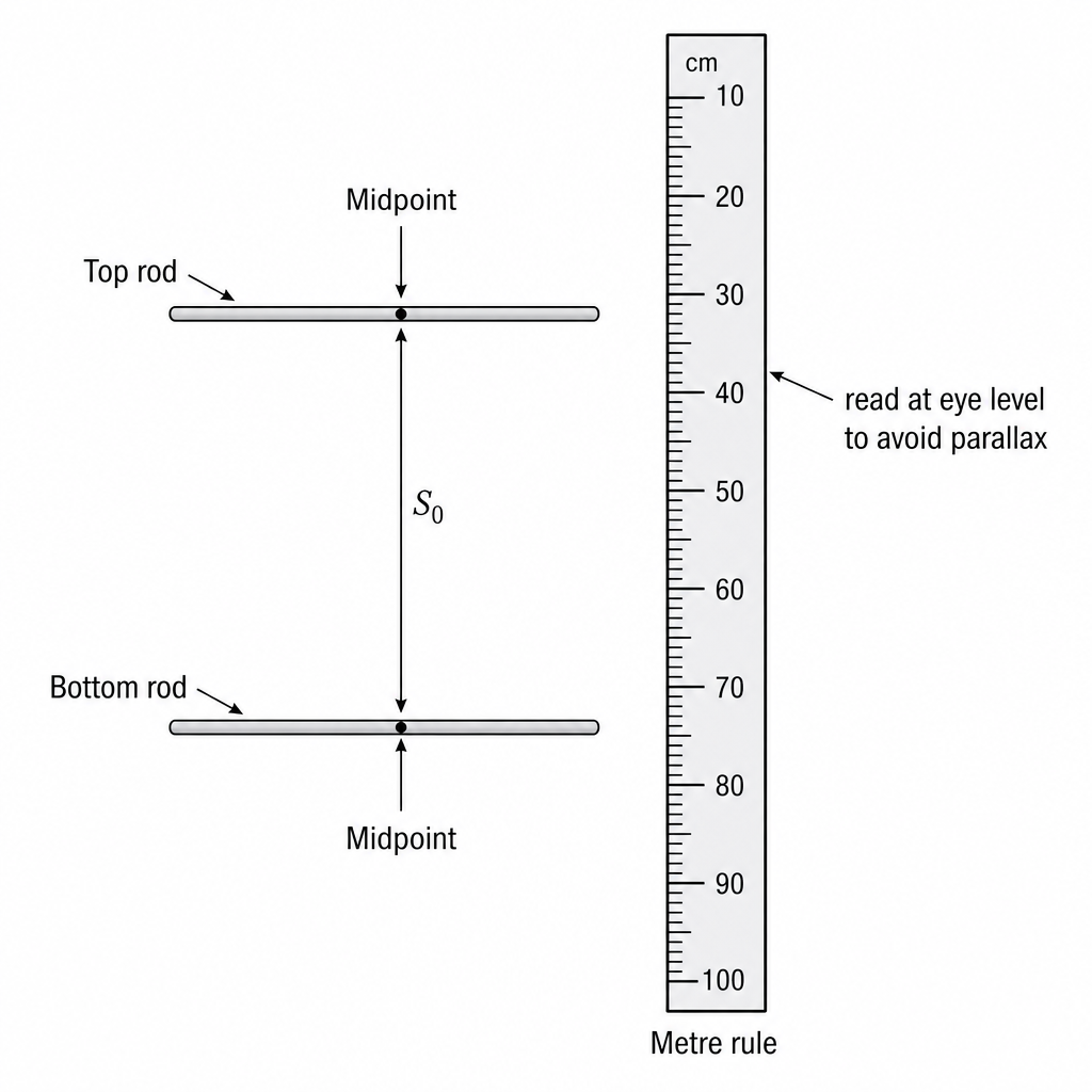
With the apparatus stationary, choose a consistent reference point on each rod (commonly the midpoints, since the string loop is at the midpoint).
Place the ruler close to the rods and vertical.
Read the separation $S_0$ at eye level.
Record $S_0$ in metres to a precision consistent with the scale (e.g. nearest $1\ \text{mm}$ gives $S_0$ to $0.001\ \text{m}$ ).

Key Takeaways

Use consistent reference points for both $S_0$ and $S_1$ .
Minimise parallax and movement during readings.

Common Mistakes

Measuring between different points for $S_0$ and $S_1$ .
Taking readings while the lower rod is still oscillating.
Forgetting to write the unit (must be $\text{m}$ here).

Things to Be Careful About

The ruler should be as close as possible to the rods; viewing from an angle introduces parallax.
Small errors in $S_0$ strongly affect $(S_1-S_0)$ , so careful reading matters.

Techniques used

assemble apparatus following the diagram and fixed distancesmeasure a vertical separation with a rule while reducing parallaxrecord a single reading with an appropriate unit and precision

(ii)

Estimate the percentage uncertainty in your value of $S_0$ . Show your working.

percentage uncertainty = ______ $\%$

1M Similar

DifficultyMedium-Easy

Worked solution

Working

(Example: metre rule resolution $= 1\ \text{mm}$ )

Absolute uncertainty in $S_0 \approx \pm 1\ \text{mm} = \pm 0.001\ \text{m}$ .

\%\ \text{uncertainty} = \frac{0.001}{0.120} \times 100 = 0.83\%

Answer

percentage uncertainty $\approx 0.8\%$

Final answer

0.8%

Detailed explanation

Background Concept

Any measurement has uncertainty. A common exam approach is to estimate the absolute uncertainty from the instrument resolution.

For a ruler with $1\ \text{mm}$ smallest division, a typical absolute uncertainty is about $\pm 1\ \text{mm}$ (sometimes $\pm 0.5\ \text{mm}$ is used; either may be acceptable depending on how you read the scale).

Percentage uncertainty is

\%\ \text{uncertainty} = \frac{\text{absolute uncertainty}}{\text{measured value}} \times 100

Understanding the Question

You must estimate the percentage uncertainty in your measured value of $S_0$ and show the working.

Approach

Decide the absolute uncertainty in $S_0$ from the measuring instrument (and reading method).
Substitute into the percentage uncertainty formula.

Step-by-Step Reasoning

If $S_0$ is read using a ruler to the nearest $1\ \text{mm}$ , take absolute uncertainty $\approx \pm 1\ \text{mm} = \pm 0.001\ \text{m}$ .
With an example value $S_0 = 0.120\ \text{m}$ :

\%\ \text{uncertainty} = \frac{0.001}{0.120}\times 100 = 0.83\%

Round suitably (often 1 s.f. or 2 s.f. is fine for uncertainties): $0.8\%$ .

Key Takeaways

Always convert absolute uncertainty into the same unit as the measurement before calculating a percentage.
Show the formula and substitution for marks.

Common Mistakes

Using $\% = \frac{S_0}{0.001}\times 100$ (inverting the fraction).
Leaving the absolute uncertainty as $1\ \text{mm}$ while $S_0$ is in metres.
Giving an uncertainty with excessive precision (e.g. $0.833333\%$ ).

Things to Be Careful About

If $S_0$ is found from two scale readings (top and bottom positions) then the absolute uncertainty may be larger (sum of the two reading uncertainties). Use the method that matches how you measured $S_0$ .

Techniques used

assign an absolute uncertainty from instrument resolutioncalculate percentage uncertainty from absolute uncertainty and measured valuequote the uncertainty to a sensible number of significant figures

(iii)

• Add a $100\text{ g}$ slotted mass to the mass hanger.
• The distance between the two rods is now $S_1$ .

Measure and record $S_1$ .

$S_1$ = ______ $\text{m}$

• The spring constant $k$ of the arrangement is given by

k = \frac{W}{S_1 - S_0}

where $W$ has the value $0.98\text{ N}$ .

Calculate $k$ .

$k$ = ______ $\text{N m}^{-1}$

1M Similar

DifficultyMedium-Easy

Worked solution

Working

(Example reading)

$S_1 = 0.170\ \text{m}$

k = \frac{W}{S_1-S_0} = \frac{0.98}{0.170-0.120} = \frac{0.98}{0.0500} = 19.6\ \text{N m}^{-1}

Answer

$S_1 = 0.170\ \text{m}$

$k = 19.6\ \text{N m}^{-1}$

Final answer

k = 19.6 N m^-1

Detailed explanation

Background Concept

For a spring (or spring arrangement) obeying Hooke’s law,

F = kx

where $F$ is the applied force, $k$ is the spring constant, and $x$ is the extension.

Here the extension is measured by the increase in separation between the rods when an additional known weight $W$ is added:

x = S_1 - S_0 qquad\Rightarrow\qquad k = \frac{W}{S_1-S_0}

Understanding the Question

After adding a $100\ \text{g}$ mass, the weight increase is given as $W = 0.98\ \text{N}$ . You must measure the new separation $S_1$ and then calculate $k$ .

Approach

Measure $S_1$ using the same method and reference points as for $S_0$ .
Compute the extension $(S_1-S_0)$ .
Substitute into $k = W/(S_1-S_0)$ .

Step-by-Step Reasoning

Use an example: $S_0 = 0.120\ \text{m}$ , $S_1 = 0.170\ \text{m}$ .
Extension:

S_1 - S_0 = 0.170 - 0.120 = 0.0500\ \text{m}

Calculate $k$ :

k = \frac{0.98}{0.0500} = 19.6\ \text{N m}^{-1}

Key Takeaways

$k$ depends on the difference $(S_1-S_0)$ , so both readings must be consistent.
Keep all lengths in metres so that $k$ comes out in $\text{N m}^{-1}$ .

Common Mistakes

Using $S_0 - S_1$ giving a negative extension.
Using $100\ \text{g}$ as $0.98\ \text{N}$ without considering that $W$ is already given.
Calculating with $S$ in cm and then forgetting to convert, giving $k$ off by a factor of 100.

Things to Be Careful About

Wait for the rod to stop moving before measuring $S_1$ .
If the ruler is not vertical, the measured separation can be too large.

Techniques used

measure a second separation after adding a known loadcalculate an extension as a difference of two measurementsapply the spring constant formula using a known weightquote the derived value with a correct unit

(c)

• The total mass hanging from the string loop is $M$ .

Record $M$ .

$M$ = ______ $\text{kg}$

• Move the lower rod a small distance downwards. Release the rod. The rod oscillates in a vertical plane.
• Take measurements to determine the period $T$ of the oscillations.

$T$ = ______ $\text{s}$

2M Similar

DifficultyMedium-Easy

Worked solution

Working

(Example values)

$M = 0.150\ \text{kg}$

Time $n = 20$ oscillations: $t = 15.2\ \text{s}$

T = \frac{t}{n} = \frac{15.2}{20} = 0.760\ \text{s}

Answer

$M = 0.150\ \text{kg}$

$T = 0.760\ \text{s}$

Final answer

T = 0.760 s

Detailed explanation

Background Concept

The period $T$ is the time taken for one complete oscillation. If you time just one oscillation with a stopwatch, reaction time causes a large percentage uncertainty. A better method is to time many oscillations and divide:

T = \frac{t}{n}

where $t$ is the total time for $n$ oscillations.

Understanding the Question

You must:

record the total hanging mass $M$ (including the mass hanger and all slotted masses),
determine the oscillation period $T$ of the lower rod.

Approach

Add up all masses to get $M$ in $\text{kg}$ .
Displace the rod slightly and release.
Use a fixed reference point and count $n$ complete oscillations.
Measure total time $t$ for $n$ oscillations, repeat, then compute $T = t/n$ .

Step-by-Step Reasoning

diagram-c-1

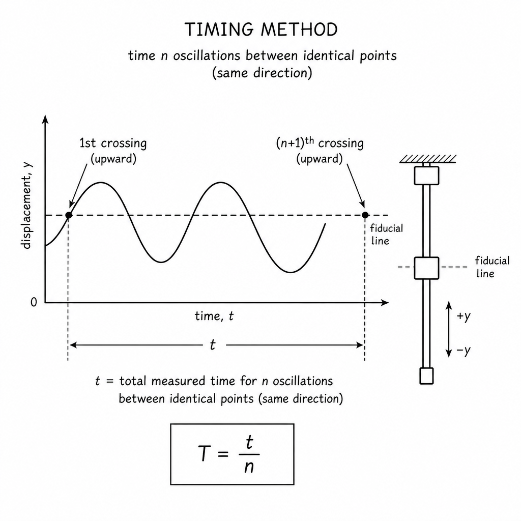
Example mass: mass hanger $0.050\ \text{kg}$ plus $0.100\ \text{kg}$ gives $M = 0.150\ \text{kg}$ .
Choose $n = 20$ oscillations to reduce timing uncertainty.
Start timing as the rod passes a fixed reference level in one direction.
Stop timing after exactly 20 complete cycles (same direction crossing).
If the time is $t = 15.2\ \text{s}$ then

T = \frac{15.2}{20} = 0.760\ \text{s}

Repeat timings and average $T$ for better reliability.

Key Takeaways

Timing many oscillations greatly reduces the percentage uncertainty in $T$ .
Always count oscillations consistently (same reference point and direction).

Common Mistakes

Timing only one oscillation.
Counting half-oscillations as full oscillations.
Starting and stopping at different reference points.
Forgetting to include the mass hanger in $M$ .

Things to Be Careful About

Keep oscillations small to better match simple harmonic motion.
Damping may make amplitude decrease; still measure over a time interval where the motion is steady and easy to count.

Techniques used

record the total suspended mass including the hangerdetermine the period by timing multiple oscillationsreduce timing uncertainty by repeating and averagingdivide total time by number of oscillations to obtain the period

(d)

• Add an additional mass of $200\text{ g}$ to the mass hanger.
• Repeat (c).

$M$ = ______ $\text{kg}$
$T$ = ______ $\text{s}$

2M Similar

DifficultyMedium-Easy

Worked solution

Working

(Example values)

$M = 0.350\ \text{kg}$

Time $n = 20$ oscillations: $t = 19.8\ \text{s}$

T = \frac{t}{n} = \frac{19.8}{20} = 0.990\ \text{s}

Answer

$M = 0.350\ \text{kg}$

$T = 0.990\ \text{s}$

Final answer

T = 0.990 s

Detailed explanation

Background Concept

For oscillations, changing the mass changes the period. To compare results fairly, the measurement technique for $T$ must be the same each time (same method, similar amplitude, and timing many oscillations).

Understanding the Question

You add an additional $200\ \text{g}$ to the mass hanger and repeat part (c): record the new total mass $M$ and measure the new period $T$ .

Approach

Compute the new $M$ by adding $0.200\ \text{kg}$ to the previous total.
Measure $T$ using the same method as before (time $n$ oscillations and divide).
Repeat the timing and average if possible.

Step-by-Step Reasoning

Example: if previously $M = 0.150\ \text{kg}$ , then after adding $0.200\ \text{kg}$ ,

M = 0.150 + 0.200 = 0.350\ \text{kg}

Time $n = 20$ oscillations. If $t = 19.8\ \text{s}$ then

T = \frac{19.8}{20} = 0.990\ \text{s}

Key Takeaways

Keep method identical between runs to make the comparison meaningful.
A larger mass typically gives a larger period.

Common Mistakes

Forgetting to update $M$ after adding mass.
Timing a different number of oscillations than in (c) and not stating it.
Changing the reference point or direction for timing.

Things to Be Careful About

Ensure the apparatus settles before timing.
Avoid sideways swinging or twisting of the rod when releasing.

Techniques used

change the independent variable by adding a known mass incrementre-measure the period using repeated timing for multiple oscillationskeep the oscillation amplitude small and consistentrecord results with consistent units and appropriate precision

(e)

It is suggested that the relationship between $T$ , $M$ , $V$ and $k$ is

\rho V = \frac{kT^2}{4\pi^2} - M

where $\rho$ is a constant.

Using your data, calculate two values of $\rho$ .

first value of $\rho$ = ______
second value of $\rho$ = ______

1M Similar

DifficultyMedium

Worked solution

Working

From

\rho V = \frac{kT^2}{4\pi^2} - M

\rho = \frac{\frac{kT^2}{4\pi^2} - M}{V}

(Using example data: $V = 1.885\times 10^{-4}\ \text{m}^3$ , $k = 19.6\ \text{N m}^{-1}$ )

First set ( $M = 0.150\ \text{kg}$ , $T = 0.760\ \text{s}$ ):

\rho_1 = \frac{\frac{19.6(0.760)^2}{4\pi^2} - 0.150}{1.885\times 10^{-4}} = 7.25\times 10^{2}\ \text{kg m}^{-3}

Second set ( $M = 0.350\ \text{kg}$ , $T = 0.990\ \text{s}$ ):

\rho_2 = \frac{\frac{19.6(0.990)^2}{4\pi^2} - 0.350}{1.885\times 10^{-4}} = 7.25\times 10^{2}\ \text{kg m}^{-3}

Answer

first value of $\rho = 7.25\times 10^{2}\ \text{kg m}^{-3}$

second value of $\rho = 7.25\times 10^{2}\ \text{kg m}^{-3}$

Final answer

ρ ≈ 7.25 × 10^2 kg m^-3 (both values, example)

Detailed explanation

Background Concept

The provided relationship is

\rho V = \frac{kT^2}{4\pi^2} - M

This resembles the mass–spring period relation

T = 2\pi\sqrt{\frac{m_{\text{effective}}}{k}} \quad\Rightarrow\quad m_{\text{effective}} = \frac{kT^2}{4\pi^2}

Here the effective oscillating mass is suggested to be $M + \rho V$ .

To find $\rho$ , rearrange:

\rho = \frac{\frac{kT^2}{4\pi^2} - M}{V}

Units check: $kT^2$ has units $(\text{N m}^{-1})(\text{s}^2) = (\text{kg s}^{-2})(\text{s}^2)=\text{kg}$ , so the numerator is kg; dividing by $V$ ( $\text{m}^3$ ) gives $\text{kg m}^{-3}$ , a density.

Understanding the Question

You have two sets of $(M, T)$ data (from parts (c) and (d)), and single values of $V$ and $k$ . You must calculate $\rho$ twice using the two different $(M,T)$ pairs.

Approach

Make $\rho$ the subject.
For each data set, calculate $\frac{kT^2}{4\pi^2}$ .
Subtract $M$ .
Divide by $V$ to obtain $\rho$ .

Step-by-Step Reasoning

Using example values from earlier parts:

$V = 1.885\times 10^{-4}\ \text{m}^3$
$k = 19.6\ \text{N m}^{-1}$

First run ( $M = 0.150\ \text{kg}$ , $T = 0.760\ \text{s}$ ):

\frac{kT^2}{4\pi^2} = \frac{19.6\times (0.760)^2}{4\pi^2} = \frac{19.6\times 0.5776}{39.48} = 0.2867\ \text{kg}

Then

\rho_1 V = 0.2867 - 0.150 = 0.1367\ \text{kg}

\rho_1 = \frac{0.1367}{1.885\times 10^{-4}} = 7.25\times 10^2\ \text{kg m}^{-3}

Second run ( $M = 0.350\ \text{kg}$ , $T = 0.990\ \text{s}$ ):

\frac{kT^2}{4\pi^2} = \frac{19.6\times (0.990)^2}{39.48} = \frac{19.6\times 0.9801}{39.48} = 0.4867\ \text{kg}

Then

\rho_2 V = 0.4867 - 0.350 = 0.1367\ \text{kg}

\rho_2 = \frac{0.1367}{1.885\times 10^{-4}} = 7.25\times 10^2\ \text{kg m}^{-3}

If your two values are close (within experimental uncertainty), it supports the suggested relationship.

Key Takeaways

Rearrangement and careful substitution are crucial.
Always check units; $\rho$ should come out in $\text{kg m}^{-3}$ .
Two consistent values of $\rho$ suggests the model fits the data.

Common Mistakes

Forgetting to divide by $V$ .
Using $4\pi$ instead of $4\pi^2$ .
Mixing units for $V$ (e.g. using $\text{cm}^3$ without converting to $\text{m}^3$ ).
Subtracting $M$ incorrectly or using the wrong $M$ with the wrong $T$ .

Things to Be Careful About

Use the same $k$ and $V$ for both calculations.
Significant figures: don’t quote $\rho$ to more precision than your measured $T$ , $S$ (hence $k$ ), and $V$ justify.

Techniques used

rearrange the given relationship to make the target quantity the subjectsubstitute measured values into the formula consistentlycalculate two independent values and compare consistencycheck units to confirm a density unit

(f)

It is suggested that the percentage uncertainty in the values of $\rho$ is $15\%$ .

Using this uncertainty, explain whether your results support the relationship in (e).

1M Similar

DifficultyMedium-Easy

Worked solution

Working

\%\ \text{difference} = \frac{|\rho_1-\rho_2|}{\frac{1}{2}(\rho_1+\rho_2)}\times 100

(Example: $\rho_1 = 7.25\times 10^2$ , $\rho_2 = 7.25\times 10^2\ \text{kg m}^{-3}$ )

\%\ \text{difference} = 0\% < 15\%

Answer

Yes. The two values of $\rho$ agree within $15\%$ , so the results support the relationship.

Final answer

Yes, they agree within 15% so the relationship is supported.

Detailed explanation

Background Concept

Experimental results are considered consistent if their difference is not larger than the stated uncertainty. A common method is to calculate the percentage difference between two values and compare it to the percentage uncertainty.

A suitable percentage difference is

\%\ \text{difference} = \frac{|\rho_1-\rho_2|}{\frac{1}{2}(\rho_1+\rho_2)}\times 100

If this is less than (or comparable to) the stated uncertainty (here $15\%$ ), the values are consistent.

Understanding the Question

You have calculated two values of $\rho$ from two different mass–period measurements. You are told the percentage uncertainty in $\rho$ is $15\%$ . You must decide whether the two values support the relationship in (e).

Approach

Compute the percentage difference between the two values of $\rho$ .
Compare it with $15\%$ .
State the conclusion: support if difference $\le 15\%$ ; do not support if difference is much larger.

Step-by-Step Reasoning

Suppose your values are $\rho_1$ and $\rho_2$ .
Calculate

\%\ \text{difference} = \frac{|\rho_1-\rho_2|}{(\rho_1+\rho_2)/2}\times 100

If (as in the example) the values are equal, the percentage difference is $0\%$ , which is well within $15\%$ .
Therefore the results are consistent with the model.

Key Takeaways

Always compare differences to uncertainty before concluding a model is wrong.
A small mismatch is expected in real experiments.

Common Mistakes

Comparing $|\rho_1-\rho_2|$ directly to $15$ (forgetting it is a percentage uncertainty).
Using $\rho_1$ alone in the denominator instead of the mean without stating.
Saying “it supports” without referencing uncertainty.

Things to Be Careful About

If your two values differ by, say, $10\%$ , that is still consistent with $15\%$ uncertainty.
If they differ by about $15\%$ , you should say it is just consistent / borderline, not “definitely” inconsistent.

Techniques used

calculate a percentage difference between two measured valuescompare the difference with a stated percentage uncertaintystate a conclusion consistent with uncertainty

(g)

(i)

Describe four sources of uncertainty or limitations of the procedure for this experiment.
For any uncertainties in measurement that you describe, you should state the quantity being measured and a reason for the uncertainty.

4M Similar

DifficultyMedium

Worked solution

Answer

Uncertainty in measuring $S_0$ and $S_1$ : difficult to align the ruler exactly vertical and read the separation without parallax; rods may not remain perfectly parallel.
Uncertainty in $(S_1-S_0)$ : it is found from the difference of two readings, so the uncertainty is larger than for a single length and can be a large fraction of the extension.
Uncertainty in $T$ : stopwatch reaction time and difficulty judging the exact instant the rod passes a reference point (especially if amplitude changes due to damping).
Uncertainty in $d$ : micrometer may have zero error and the rod diameter may not be perfectly uniform/circular, so a single measurement of $d$ may not represent the true mean diameter.

Final answer

Four limitations/uncertainties listed (S readings/parallax, difference S1-S0, timing T reaction, diameter d zero error/non-uniformity).

Detailed explanation

Background Concept

In practical work, uncertainty arises from:

instrument resolution and reading technique (parallax),
repeatability (scatter between repeats),
systematic errors (zero error, calibration),
experimental limitations (damping, unwanted motion).

This question wants four distinct sources and, when it is a measurement uncertainty, it must name the quantity and explain why it is uncertain.

Understanding the Question

You must critique the procedure: what parts of measuring $L$ , $d$ , $S_0$ , $S_1$ , and $T$ are difficult or imprecise, and why that affects the final calculated values ( $k$ and $\rho$ ).

Approach

List four clear points. For each:

name the quantity (e.g. $S_0$ , $T$ , $d$ ),
state the physical reason (parallax, motion, zero error, non-uniform shape, damping),
indicate the consequence (affects $S_1-S_0$ , affects $k$ , affects $\rho$ ).

Step-by-Step Reasoning

Separation measurements $S_0$ and $S_1$
- The distance is vertical; if the ruler is not vertical or not close to the rods, the reading changes.
- Parallax occurs if the scale is read at an angle.
- The rods may not be perfectly parallel, so separation can vary along their length.
Extension found by subtraction $(S_1-S_0)$
- Even if each of $S_0$ and $S_1$ is measured to about $\pm 1\ \text{mm}$ , the extension (difference) can have uncertainty closer to $\pm 2\ \text{mm}$ .
- If the extension is small, this becomes a large percentage uncertainty in $k$ .
Timing the period $T$
- Human reaction time in starting/stopping the stopwatch introduces uncertainty.
- If the oscillations are damped, the amplitude decreases and it is harder to decide when a cycle is complete.
- Any sideways swinging or twisting makes identifying a consistent reference point harder.
Diameter $d$ measurement
- Micrometers can have zero error; if not checked, all readings shift systematically.
- The rod may not be perfectly circular or may vary along its length; a single reading can be unrepresentative, affecting $V$ .

Any four well-explained, distinct limitations like these gain credit.

Key Takeaways

Good limitation statements always identify the measured quantity and the reason.
Differences of readings (like $S_1-S_0$ ) often dominate uncertainty.

Common Mistakes

Writing vague statements like “human error” with no quantity and no mechanism.
Repeating the same idea in different words (e.g. parallax twice) instead of four distinct sources.
Giving improvements instead of limitations (that belongs in (g)(ii)).

Things to Be Careful About

Ensure each of the four points is genuinely different.
Prioritise limitations that strongly affect $k$ , $T$ , $V$ , and thus $\rho$ .

Techniques used

identify specific measurements that dominate uncertaintylink each limitation to a physical cause of errordescribe how the limitation affects the measured quantitiesstate multiple distinct uncertainty sources

(ii)

Describe four improvements that could be made to this experiment. You may suggest the use of other apparatus or different procedures.

4M Similar

DifficultyMedium

Worked solution

Answer

Measure $S_0$ and $S_1$ with a fixed vertical scale and a pointer/fiducial marker on the lower rod (or use a set square) to reduce parallax and ensure the separation is read consistently.
Increase the extension by using a larger known added mass (still within elastic limit) so that $(S_1-S_0)$ is larger, reducing percentage uncertainty in $k$ .
Determine $T$ using a light gate/motion sensor/data logger (or video analysis) instead of a stopwatch to remove reaction-time uncertainty.
Measure $d$ at several positions and in two perpendicular directions, apply any micrometer zero correction, and take the mean value to improve the estimate of $V$ .

Final answer

Four improvements listed (fiducial/pointer for S, larger extension, data logging for T, multiple d measurements with zero correction).

Detailed explanation

Background Concept

Improvements are changes that reduce uncertainty, reduce systematic error, or increase reliability. Strong improvements:

directly target a stated limitation,
are practical and clearly described,
explain what quantity becomes more accurate.

Understanding the Question

You must propose four improvements to make measurements of $S_0$ , $S_1$ , $T$ , $L$ , $d$ , and derived quantities ( $k$ , $\rho$ ) more reliable/accurate.

Approach

Take the main limitation sources (parallax in $S$ , subtraction uncertainty in $S_1-S_0$ , reaction time in $T$ , non-uniform $d$ ) and propose a fix for each.

Step-by-Step Reasoning

Improve $S$ measurements (reduce parallax and inconsistency)
- Attach a pointer to the lower rod and read against a fixed vertical scale.
- Use a set square to ensure the reading is taken horizontally from the pointer to the scale.
Reduce percentage uncertainty in $k$
- Make the extension larger by using a larger added load to obtain $S_1-S_0$ (staying within the elastic limit).
- Alternatively, take several load values and plot $W$ against extension; gradient gives $k$ and averages out random error.
Improve timing for $T$
- Use electronic timing (light gate, motion sensor, data logger) to avoid human reaction time.
- If using a stopwatch, time many oscillations and repeat several times, then average.
Improve $V$ (hence $\rho$ ) by better $d$ measurements
- Check micrometer zero error and correct readings.
- Measure $d$ at multiple positions and orientations and take the mean.

Key Takeaways

The best improvements are specific and linked to the physics and measurements.
Using electronic sensors is a strong way to improve timing.

Common Mistakes

Suggesting improvements that don’t change uncertainty (e.g. “be more careful”).
Giving fewer than four improvements or repeating the same idea.
Proposing unrealistic apparatus without explaining how it would be used.

Things to Be Careful About

If suggesting larger loads, explicitly note the springs must remain within elastic limit.
If suggesting more readings, state clearly what you would repeat/average (e.g. repeat timings of $n$ oscillations; measure $d$ at several points).

Techniques used

propose apparatus changes that reduce identified uncertaintiesmatch each improvement to a specific limitationincrease reliability by repeats and averagingreduce parallax by using fiducial markers or fixed scales