In this experiment, you will investigate oscillations. (a) You have been provided with a board of width $w$ and thickness $x$, as shown in Fig. 2.1. Measure and record $w$ and $x$. $w$ = \_\_\_\_\_\_ $x$ = \_\_\_\_\_\_ (i) • Set up the apparatus as shown in Fig. 2.2. • Ensure the rods of the clamps are the same height above the bench. • Slide the rods of the clamps through the holes in the board as shown in Fig. 2.2. Ensure that each end of the board touches a stand. • The…

(a) w = 5.0 cm, x = 0.60 cm (example) · (b)(i) d = 95.0 cm (example) · (b)(ii) 0.11% · (c) T = 1.65 s (example) · (d) d = 70.0 cm, T = 1.40 s (example) · (e)(i) k1 = 1.0×10^-2 s cm^-1, k2 = 1.0×10^-2 s cm^-1 (example) · (e)(ii) k to 2 s.f. (limited by T−a, with a = 0.70 s) · (f) Yes, supports (k values agree within 10%). · (g)(i) Four valid uncertainties/limitations listed (see solution). · (g)(ii) Four valid improvements listed (see solution).

Physics 9702/31 — October/November 2024

Cambridge AS Level · Advanced Practical Skills · worked solutions for every part, with the mark scheme

questions

marks

120

minutes

Topics Manipulation, Measurement and Observation · Presentation of Data and Observations · Analysis, Conclusions and Evaluation

Q1MediumManipulation, Measurement and ObservationPresentation of Data and ObservationsAnalysis, Conclusions and Evaluation

In this experiment, you will investigate the equilibrium position of a wooden strip.

Some of the apparatus has been set up for you.

(a)

• Set up the apparatus as shown in Fig. 1.1.

Fig. 1.1

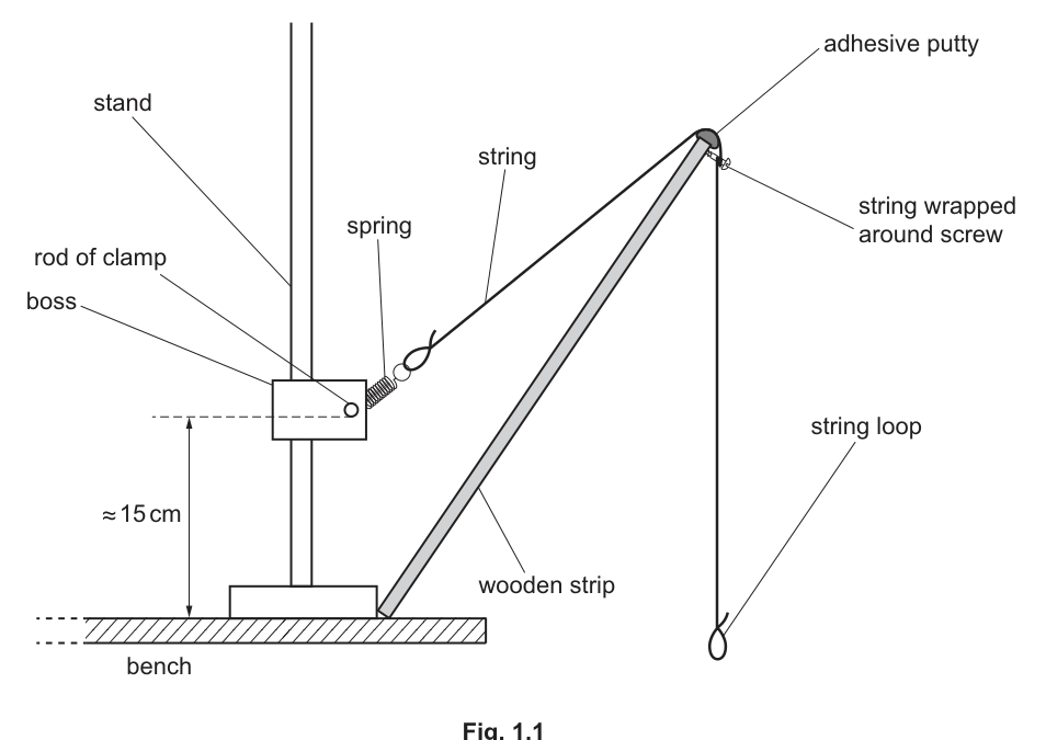
• Ensure the rod of the clamp is approximately $15\text{ cm}$ above the bench.
• Arrange the wooden strip so that the bottom of the strip rests against the base of the stand.
• Use adhesive putty to fix the string centrally on the wooden strip in line with the spring.
• Wrap the string around the screw.

• Arrange the block and protractor as shown in Fig. 1.2.

Fig. 1.2

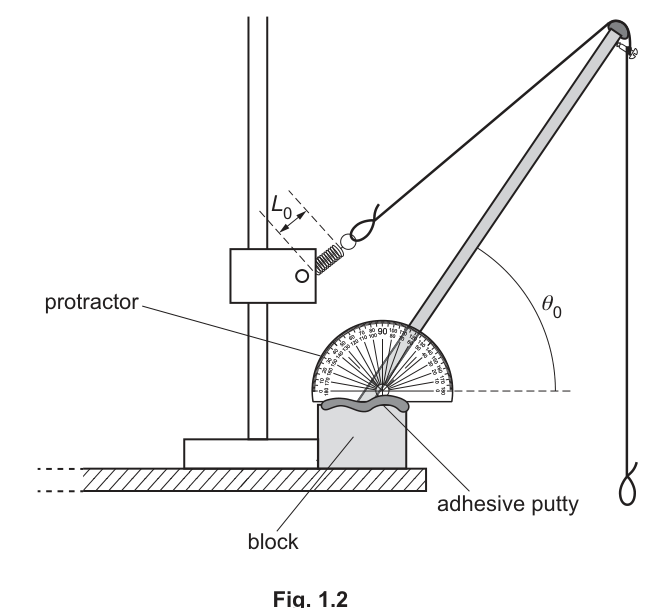
• The length of the coiled section of the spring is $L_0$ , as shown in Fig. 1.2.

The angle between the lower edge of the wooden strip and the horizontal is $\theta_0$ , as shown in Fig. 1.2.

Adjust the apparatus until $\theta_0$ is between $75^\circ$ and $85^\circ$ . You may wish to move the protractor along the block.

• Measure and record $L_0$ and $\theta_0$ .

$L_0$ = ______
$\theta_0$ = ______ $^\circ$

1M Similar

DifficultyEasy

Worked solution

Answer

Measure $L_0$ (length of coiled section) with a rule and record it to suitable precision (e.g. nearest $1\ \text{mm}$ ).

Adjust so that $75^\circ \le \theta_0 \le 85^\circ$ , then read $\theta_0$ from the protractor and record it (e.g. to the nearest $1^\circ$ ).

Example recorded values (student-dependent):

$L_0 = 3.8\ \text{cm}$

$\theta_0 = 80^\circ$

Final answer

Student-dependent (e.g. L0 = 3.8 cm, θ0 = 80°)

Detailed explanation

Background Concept

This part tests careful experimental set-up and direct measurement. A length measurement should be taken with the scale aligned to the quantity being measured (here, the coiled/active section of the spring), and an angle should be read from a protractor using the correct reference line (here, the lower edge of the strip) and the correct baseline (the horizontal).

Understanding the Question

You are told exactly how the apparatus should be arranged (strip against the base, spring and string attached centrally, protractor on the block). You must then adjust until the starting angle $\theta_0$ lies between $75^\circ$ and $85^\circ$ , and record the corresponding spring length $L_0$ and angle $\theta_0$ .

Approach

Assemble the apparatus exactly as shown and ensure the clamp rod height is about $15\ \text{cm}$ .
Slide/position the protractor so you can read the angle between the strip’s lower edge and the horizontal.
Adjust until the angle is in the given range.
Read and record $L_0$ and $\theta_0$ with appropriate precision.

Step-by-Step Reasoning

Set the strip so its bottom rests against the stand base (this fixes the contact point and helps repeatability).
Fix the string centrally (reduces twisting/sideways forces).
Place the protractor on the block so the baseline is horizontal; align the strip’s lower edge with the protractor scale.
Adjust the system until $\theta_0$ is between $75^\circ$ and $85^\circ$ .
Measure $L_0$ as the length of the coiled section only (not including hooks/loops if they are not part of the coiled section).
Record $L_0$ to the precision of the ruler (typically nearest $1\ \text{mm}$ ) and $\theta_0$ to the protractor’s resolution (typically nearest $1^\circ$ ).

Key Takeaways

Follow the specified geometry before taking readings.
Always match the recorded precision to the measuring instrument.

Common Mistakes

Measuring the total spring length including end loops instead of just the coiled section.
Reading the protractor from the wrong scale (inside vs outside) or using the wrong reference line.
Recording an angle outside the required range $75^\circ$ to $85^\circ$ .

Things to Be Careful About

Avoid parallax: keep your eye directly above the ruler/protractor marking.
Ensure the protractor baseline is truly horizontal (use the top face of the block as the horizontal reference).
Record units: $L_0$ needs a length unit; $\theta_0$ must be in degrees.

Techniques used

set up the apparatus to match the diagram and specified geometryread a length from a rule aligned with the spring coilsread an angle from a protractor with the correct reference line

(b)

• Make a hook from one paper clip and hang nine paper clips from it as shown in Fig. 1.3.

Fig. 1.3

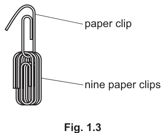
• The mass of all ten paper clips is $m$ .

Measure and record $m$ .

$m$ = ______

1M Similar

(c)

• Using the mass hanger and slotted masses, hang a mass of $40\text{ g}$ from the string loop.

• Hang the paper clips from the string loop as shown in Fig. 1.4.

Fig. 1.4

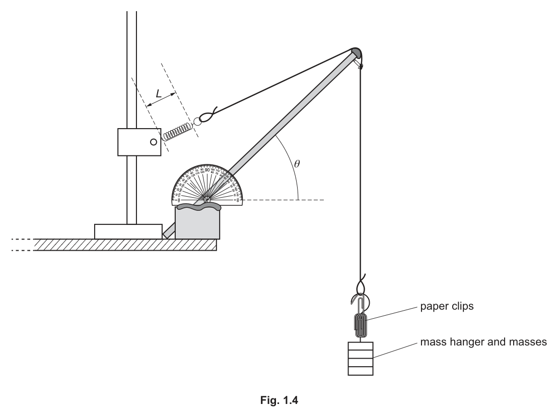
• The total mass hanging from the string loop is $M$ .

The angle between the wooden strip and the horizontal is $\theta$ , as shown in Fig. 1.4.

The length of the coiled section of the spring is $L$ , as shown in Fig. 1.4.

Determine and record $M$ .

$M$ = ______

• Measure and record $\theta$ and $L$ .

$\theta$ = ______ $^\circ$
$L$ = ______

• Calculate $e$ where

e = (L - L_0)

$e$ = ______

1M Similar

DifficultyMedium-Easy

Worked solution

Working

Total hanging mass

M = (40\ \text{g}) + m

Measure $\theta$ and $L$ .

e = (L - L_0)

Example values (student-dependent):

If $m = 8.6\ \text{g}$ , then

M = 48.6\ \text{g}

If $L = 5.1\ \text{cm}$ and $L_0 = 3.8\ \text{cm}$ ,

e = 1.3\ \text{cm}

Answer

$M = 48.6\ \text{g}$ , $\theta = 72^\circ$ , $L = 5.1\ \text{cm}$ , $e = 1.3\ \text{cm}$ (example only; student-dependent).

Final answer

Student-dependent (compute M; measure θ, L; e = L − L0)

Detailed explanation

Background Concept

This part uses the idea of extension of a spring-like element: extension is the change in length from an initial reference length.

e = L - L_0

Here, $L_0$ is the initial length of the coiled section, and $L$ is the new length after adding a known load. The total load is described by a total mass $M$ .

Understanding the Question

You must:

Add a fixed $40\ \text{g}$ mass to the string loop.
Also hang the ten paper clips from the string loop.
Determine the total hanging mass $M$ .
Measure the new angle $\theta$ and spring coiled length $L$ .
Calculate the extension $e$ using $e = (L - L_0)$ .

Approach

Compute $M$ by adding the masses of everything hanging from the string loop.
Take fresh readings of $\theta$ and $L$ once the system is at rest.
Subtract the initial length $L_0$ to obtain $e$ .

Step-by-Step Reasoning

The $40\ \text{g}$ comes from the mass hanger plus slotted masses used to make a total of $40\ \text{g}$ .
The paper clips have mass $m$ measured in part (b).
Therefore the total hanging mass is:

M = 40\ \text{g} + m

Allow the system to settle so the strip is stationary (equilibrium).
Read $\theta$ on the protractor using the same reference (lower edge of strip vs horizontal).
Measure $L$ as the coiled length of the spring (same definition as $L_0$ ).
Compute extension:

e = L - L_0

Record $e$ to the same precision as $L$ and $L_0$ (since subtraction limits precision).

Key Takeaways

Total mass is the sum of all masses hanging.
Extension is a difference, so consistent length definition and consistent precision matter.

Common Mistakes

Forgetting to include the paper clips in $M$ , or double-counting masses.
Using different reference points for $L$ and $L_0$ (e.g. measuring to different ends).
Calculating $e$ as $L_0 - L$ (wrong sign).

Things to Be Careful About

Ensure the load hangs freely and does not touch the stand or strip.
Let oscillations die away before reading $\theta$ and $L$ .
Keep units consistent: if $L$ and $L_0$ are in $\text{cm}$ , then $e$ is in $\text{cm}$ .

Techniques used

determine a total mass by summing component massesmeasure angle and length from the apparatuscalculate an extension using a difference of lengths

(d)

Vary $M$ . The total mass $M$ may be made from slotted masses only or from $m$ and slotted masses. For each value of $M$ , measure and record $M$ , $\theta$ and $L$ . Repeat until you have six sets of values.

Record your results in a table. Include values of $e$ and $\sin\theta$ in your table.

9M Similar

DifficultyMedium

Worked solution

Answer

Take six different values of total mass $M$ (using slotted masses and/or adding the paper clips), and for each value measure $\theta$ and $L$ .

Calculate for each set:

e = L - L_0

and

\sin\theta

Record all results in one table with clear headings including units, for example:

$M\ /\ \text{g}$	$\theta\ /\ ^\circ$	$L\ /\ \text{cm}$	$e\ /\ \text{cm}$	$\sin\theta$
(e.g.) $48.6$	$72$	$5.1$	$1.3$	$0.951$

(Values are examples only; your six sets must be your own readings.)

Final answer

Table of 6 sets of M, θ, L plus calculated e and sinθ (student-dependent)

Detailed explanation

Background Concept

In Paper 3, marks for tables are awarded for: a sufficient number of readings, a sensible range of the independent variable, correct and consistent recording of raw data, and correct calculation of derived quantities. Here, you are building a data set to later test a linear relationship between $e$ and $\sin\theta$ .

Understanding the Question

You must:

Change the load $M$ repeatedly.
For each $M$ , measure $\theta$ and $L$ .
Do this until you have six sets of values.
Present the results in a single table that also includes calculated columns for $e$ and $\sin\theta$ .

Approach

Choose six values of $M$ spanning a reasonable range (not all close together).
For each $M$ , let the system settle, then read $\theta$ and measure $L$ .
Compute $e$ using the fixed $L_0$ measured in (a).
Compute $\sin\theta$ (calculator in degree mode).
Put everything into a single table with quantity/unit headings and consistent precision.

Step-by-Step Reasoning

Decide your six masses (for example increasing in equal steps). You may either:
- use slotted masses only, or
- use slotted masses plus the paper clips (adding $m$ to the total).
For each chosen $M$ $M$ :
- check the mass is hanging freely,
- wait until the strip is at rest,
- measure $\theta$ to the nearest degree,
- measure $L$ to the nearest millimetre.
Calculate extension for each reading using the same $L_0$ each time:

e = L - L_0

Calculate $\sin\theta$ for each angle (ensure degrees, not radians):

\sin\theta

Construct a results table:
- all data in one table (not multiple small tables),
- headings must include the quantity symbol and unit where applicable (e.g. $L\ /\ \text{cm}$ , not just “ $L$ ”),
- raw data columns should have consistent decimal places (e.g. all $L$ values to $0.1\ \text{cm}$ if using a mm rule),
- derived quantities should be to a sensible number of significant figures (e.g. $\sin\theta$ to 3 s.f.).

Key Takeaways

Good data needs: enough points (six), a range, and clear consistent recording.
Derived columns ( $e$ and $\sin\theta$ ) must be calculated correctly and presented clearly.

Common Mistakes

Fewer than six sets of results.
No units in the table headings.
Inconsistent precision in a column (e.g. mixing $5.1$ and $5.12$ for $L$ ).
Calculating $\sin\theta$ with the calculator in radian mode.
Re-measuring $L_0$ each time (it should stay as the initial reference unless instructed otherwise).

Things to Be Careful About

Choose a sensible spread of $M$ so $\theta$ changes noticeably; otherwise the graph later will be poor.
Keep the definition of $L$ consistent (same endpoints each time).
Since $e$ comes from subtraction, record $L$ and $L_0$ to the same decimal place so $e$ is meaningful.

Techniques used

vary the independent variable over a suitable rangerecord raw measurements in a well-structured table with unitscalculate derived quantities from measured datamaintain consistent significant figures within each table column

(e)

(i)

Plot a graph of $e$ on the $y$ -axis against $\sin\theta$ on the $x$ -axis.

3M Similar

DifficultyMedium-Easy

Worked solution

Answer

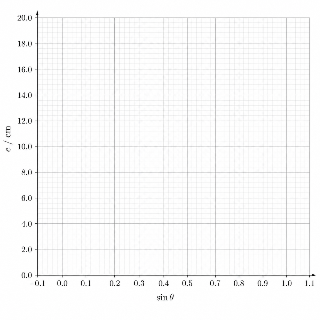
Plot $e$ on the $y$ -axis against $\sin\theta$ on the $x$ -axis.

Label axes as $e$ (with unit) and $\sin\theta$ (no unit).
Use a sensible scale so the plotted points occupy at least half the grid in both directions.
Plot all six points accurately as crosses.

Final answer

Graph of e (y) against sinθ (x)

Detailed explanation

Background Concept

A graph is used to reveal relationships between variables. Correct graph technique is assessed by: correct variables on correct axes, correct axis labels (including units), sensible scales, accurate plotting, and using all data points.

Understanding the Question

From your table in (d), you now have six values of $e$ and the corresponding $\sin\theta$ . You must plot a graph with $e$ on the vertical axis and $\sin\theta$ on the horizontal axis.

Approach

Decide on axis limits based on the minimum and maximum of your data.
Choose scales that are easy to plot (1, 2, 5, 10 per big square, etc.) and that use much of the grid.
Label axes properly.
Plot each data pair $(\sin\theta, e)$ accurately.

Step-by-Step Reasoning

Read the range of $\sin\theta$ values from your table (likely close to 1 if $\theta$ is large).
Read the range of $e$ values.
Draw axes and label:
- horizontal: $\sin\theta$ (dimensionless, so no unit),
- vertical: $e$ with the unit you used for length (e.g. $e\ /\ \text{cm}$ ).
Choose scales so that the points are spread out.
Plot each point carefully: go to the correct $x$ value ( $\sin\theta$ ), then up to the correct $y$ value ( $e$ ).

graph-axes-e-vs-sin

Key Takeaways

Axis labels must include quantity and unit (except for dimensionless quantities).
Good scales make trends clear and improve the accuracy of later gradient calculations.

Common Mistakes

Swapping axes (plotting $\sin\theta$ on $y$ instead of $x$ ).
Writing the wrong label such as “ $\theta$ ” instead of “ $\sin\theta$ ”.
Using a cramped scale so points occupy only a small portion of the grid.

Things to Be Careful About

$\sin\theta$ has no unit.
Plot points as small crosses; do not join dot-to-dot.
Ensure you plot all six points, not just a selection.

Techniques used

choose suitable axis scales to use most of the graph gridlabel axes with quantity and unitplot points accurately from a results table

(ii)

Draw the straight line of best fit.

1M Similar

(iii)

Determine the gradient and $y$ -intercept of this line.

gradient = ______
$y$ -intercept = ______

2M Similar

DifficultyMedium-Easy

Worked solution

Working

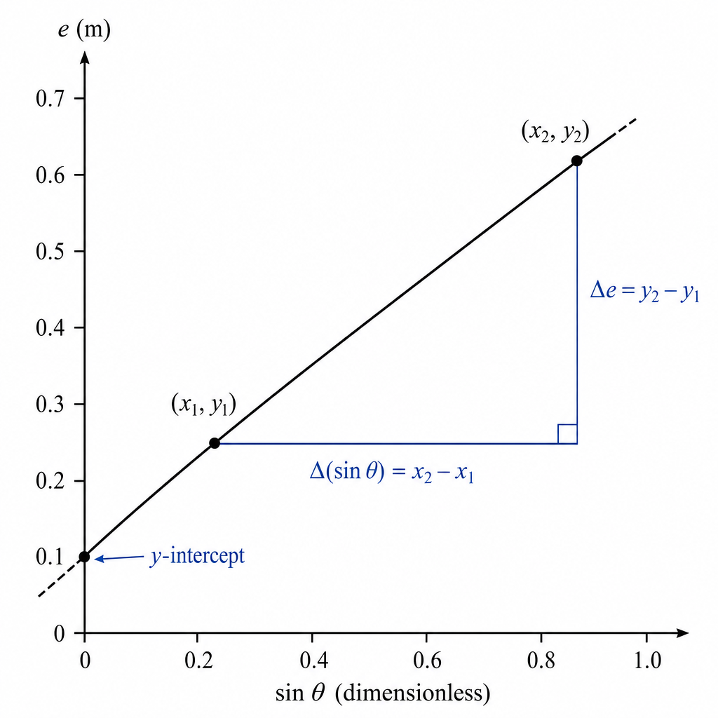
Choose two points on the best-fit line well separated in $x$ .

\text{gradient} = \frac{\Delta e}{\Delta (\sin\theta)}

Read the $y$ -intercept at $\sin\theta = 0$ from where the best-fit line crosses the $e$ -axis.

Example (student-dependent):

\text{gradient} = 4.2\ \text{cm}

\text{$y$-intercept} = -2.6\ \text{cm}

Answer

gradient $= \dfrac{\Delta e}{\Delta (\sin\theta)}$ and $y$ -intercept is the value of $e$ when $\sin\theta = 0$ (values from your graph).

Final answer

Student-dependent (gradient and y-intercept from best-fit line)

Detailed explanation

Background Concept

For a straight-line graph of the form $y = mx + c$ :

the gradient $m$ is the change in $y$ per change in $x$ :

m = \frac{\Delta y}{\Delta x}

the $y$ -intercept $c$ is the value of $y$ when $x = 0$ .

In this question, $y \equiv e$ and $x \equiv \sin\theta$ .

Understanding the Question

You must extract two numbers from your best-fit line on the $e$ vs $\sin\theta$ graph:

the gradient (slope),
the $y$ -intercept.

These will later be used to find constants in a proposed equation.

Approach

Use a large gradient triangle: pick two points far apart on the best-fit line (not necessarily data points).
Compute the gradient as $\Delta e / \Delta(\sin\theta)$ .
Find the intercept by extending the best-fit line to cross the $e$ -axis at $\sin\theta = 0$ .

Step-by-Step Reasoning

Gradient

Mark two points on the best-fit line that are far apart to reduce percentage uncertainty.
Read their coordinates: $(x_1, y_1)$ and $(x_2, y_2)$ where $x = \sin\theta$ and $y = e$ .
Calculate:

\text{gradient} = \frac{y_2 - y_1}{x_2 - x_1} = \frac{\Delta e}{\Delta (\sin\theta)}

Units: $\sin\theta$ is dimensionless, so the gradient has the same unit as $e$ (a length).

$y$ -intercept

Extend the best-fit line back to $x = 0$ (i.e. $\sin\theta = 0$ ).
Read off the corresponding $e$ value. This is the $y$ -intercept.

gradient-triangle

Key Takeaways

Always use points on the best-fit line (not point-to-point) and a large triangle.
Gradient units follow from $\text{units of }y / \text{units of }x$ .

Common Mistakes

Using two neighbouring points, giving a small triangle and an inaccurate gradient.
Calculating $\Delta x / \Delta y$ instead of $\Delta y / \Delta x$ .
Reading the intercept at $\sin\theta = 1$ instead of $0$ .

Things to Be Careful About

Do not force the line through the origin unless the plotted trend clearly requires it.
Keep enough significant figures from the graph reading (typically 2–3 s.f. for gradient/intercept).
If your graph does not extend to $\sin\theta = 0$ , you may need to extrapolate; do this carefully with a thin best-fit line.

Techniques used

select two well-separated points on the best-fit linecalculate a gradient using \Delta y / \Delta xread the y-intercept from the graph at x = 0

(f)

It is suggested that the quantities $e$ and $\theta$ are related by the equation

e = P \sin\theta + Q

where $P$ and $Q$ are constants.

Using your answers in (e)(iii), determine the values of $P$ and $Q$ .
Give appropriate units.

$P$ = ______
$Q$ = ______

2M Similar

DifficultyMedium-Easy

Worked solution

Working

Given

e = P\sin\theta + Q

Compare with $y = mx + c$ for a graph of $e$ (y-axis) against $\sin\theta$ (x-axis).

P = \text{gradient}

Q = \text{$y$-intercept}

Units: since $\sin\theta$ is dimensionless, $P$ has the same unit as $e$ and $Q$ has the same unit as $e$ .

Answer

$P =$ gradient (unit of length, e.g. $\text{cm}$ ).

$Q =$ $y$ -intercept (unit of length, e.g. $\text{cm}$ ).

Final answer

P = gradient, Q = y-intercept (both with length units)

Detailed explanation

Background Concept

A straight-line relationship can be written as:

y = mx + c

where $m$ is the gradient and $c$ is the $y$ -intercept. If you plot the correct variables, the constants in the physical equation can be read directly from the graph.

Understanding the Question

You are told:

e = P\sin\theta + Q

You already plotted $e$ (vertical) against $\sin\theta$ (horizontal) and found the gradient and intercept in (e)(iii). You must now state the numerical values of $P$ and $Q$ and include appropriate units.

Approach

Match the suggested equation to $y = mx + c$ by identifying:

$y \equiv e$
$x \equiv \sin\theta$
Then read off:
$P$ as the gradient
$Q$ as the intercept
Finally decide units from the graph/definition of variables.

Step-by-Step Reasoning

Write the proposed equation in the same pattern as $y = mx + c$ :

e = P(\sin\theta) + Q

Since your graph has $e$ on the $y$ -axis and $\sin\theta$ on the $x$ -axis, the best-fit line equation is:

e = (\text{gradient})\, (\sin\theta) + (\text{$y$-intercept})

Therefore:

P = \text{gradient}

and

Q = \text{$y$-intercept}

Units:
- $\sin\theta$ is dimensionless.
- $e$ is a length (same units as $L$ and $L_0$ ).
- So $P$ must have units of length, and $Q$ must also have units of length.

Key Takeaways

Plotting the right variables makes constants easy to obtain.
Dimensionless quantities do not change units when multiplying.

Common Mistakes

Swapping $P$ and $Q$ .
Giving $P$ units like $\text{cm}^{-1}$ or adding an extra unit from $\sin\theta$ (it has none).
Quoting $P$ and $Q$ in different length units from those used for $e$ .

Things to Be Careful About

Use the gradient and intercept from your best-fit line, not from joining two data points.
Keep units consistent with your graph axis label for $e$ (e.g. if $e$ is in $\text{mm}$ , then $P$ and $Q$ should be in $\text{mm}$ ).

Techniques used

compare a proposed linear equation to y = mx + cidentify constants from the gradient and interceptassign units by dimensional reasoning

Q21MMediumManipulation, Measurement and ObservationAnalysis, Conclusions and EvaluationPresentation of Data and Observations

In this experiment, you will investigate oscillations.

(a)

You have been provided with a board of width $w$ and thickness $x$ , as shown in Fig. 2.1.

Fig. 2.1

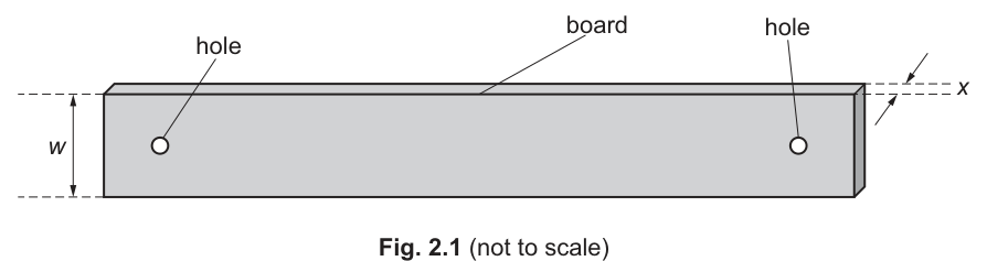
Measure and record $w$ and $x$ .

$w$ = ______
$x$ = ______

1M Similar

DifficultyEasy

Worked solution

Answer

(Example readings to suitable precision)

$w = 5.0\ \text{cm}$

$x = 0.60\ \text{cm}$

Final answer

w = 5.0 cm, x = 0.60 cm (example)

Detailed explanation

Background Concept

In practical work, the mark is usually for (i) using appropriate apparatus and (ii) recording the reading with a precision that matches the instrument. A ruler with 1 mm divisions has a typical reading uncertainty of about (\pm 0.5\ \text{mm}) for a single reading, and readings should be recorded to the nearest mm (i.e. (0.1\ \text{cm})) or nearest (0.01\ \text{m}) as appropriate.

Understanding the Question

You are given a board. You must measure its width (w) and thickness (x), as labelled in Fig. 2.1, and record both values.

Approach

Choose a suitable instrument: a ruler is usually sufficient; vernier calipers can improve the thickness measurement.
Take each measurement carefully (avoid parallax; ensure the ruler is aligned with the correct edges).
Record the values with units and with a sensible number of decimal places.

Step-by-Step Reasoning

Place the board flat and measure (w) across the labelled width, ensuring the ruler’s zero is aligned with one edge.
Measure (x) (thickness) by placing the board edge-on and measuring the separation between the two faces.
Record both in (\text{cm}) with a precision consistent with the scale divisions (e.g. to (0.1\ \text{cm}) for a mm ruler).

Key Takeaways

Record measurements to match instrument resolution.
Always include units.
Avoid parallax and misalignment.

Common Mistakes

Missing units.
Recording too many decimal places (e.g. (5.000\ \text{cm}) with a ruler).
Measuring the wrong dimension (e.g. confusing thickness and width).

Things to Be Careful About

Check the labelled dimension carefully: (w) is the width of the board, (x) is the thickness.
Ensure the ruler is not tilted; read at eye level to reduce parallax.
If using calipers, ensure they are zeroed before measuring.

Techniques used

measure lengths with a ruler or calipers to an appropriate precisionavoid parallax by viewing the scale perpendicularlyrecord values with consistent decimal places matching instrument resolution

(b)

(i)

• Set up the apparatus as shown in Fig. 2.2.

Fig. 2.2

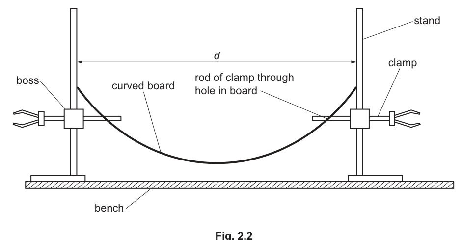
• Ensure the rods of the clamps are the same height above the bench.
• Slide the rods of the clamps through the holes in the board as shown in Fig. 2.2. Ensure that each end of the board touches a stand.
• The distance between the inside edges of the stands is $d$ , as shown in Fig. 2.2. Adjust the apparatus until $d$ is in the range $92\text{ cm}$ to $99\text{ cm}$ .
• Measure and record $d$ .

$d$ = ______ $\text{cm}$

2M Similar

DifficultyMedium-Easy

Worked solution

Answer

(Example value in the required range)

$d = 95.0\ \text{cm}$

Final answer

d = 95.0 cm (example)

Detailed explanation

Background Concept

In Paper 3, marks for a set-up/measurement step are earned by following the stated constraints (e.g. a range for (d)) and taking a measurement consistently from the defined reference points (here, the inside edges of the stands).

Understanding the Question

You must assemble the apparatus as in Fig. 2.2 and then adjust it so that (d) (the distance between the inside edges of the stands) is between (92\ \text{cm}) and (99\ \text{cm}). Then you measure and record (d).

Approach

Build the arrangement so the board is supported symmetrically.
Ensure both clamp rods are at the same height (so the board bends symmetrically).
Measure (d) between the specified points (inside edges), and record it with appropriate precision.

Step-by-Step Reasoning

Set up the two stands and clamps; adjust until the rods are level with each other.
Thread the rods through the board’s holes and ensure each end of the board touches a stand.
Use a metre rule to measure the distance between the inside faces/edges of the stands.
Adjust stand separation until (92\le d \le 99\ \text{cm}), then record (d) to the nearest mm ((0.1\ \text{cm})) if using a mm-scale ruler.

Key Takeaways

Always measure from the stated reference points.
Check the required range before recording.
Symmetry and level supports improve repeatability.

Common Mistakes

Measuring between the outside edges instead of inside edges.
Measuring at an angle (not perpendicular), giving a larger value.
Not ensuring the clamp rods are at the same height.

Things to Be Careful About

Keep the ruler parallel to the line joining the stands.
Ensure the board ends are actually touching the stands, as stated.
Record (d) with unit (\text{cm}) and consistent precision.

Techniques used

set up apparatus to a diagram with correct alignmentmeasure a separation between reference points consistentlycheck the measurement lies within a stated acceptable range

(ii)

Estimate the percentage uncertainty in your value of $d$ . Show your working.

percentage uncertainty = ______ %

1M Similar

DifficultyMedium-Easy

Worked solution

Working

(Example using a metre rule with 1 mm resolution)

Take absolute uncertainty in $d$ as $\pm 0.10\ \text{cm}$ .

\%\ \text{uncertainty} = \frac{0.10}{95.0} \times 100 = 0.105\% \approx 0.11\%

Answer

$0.11\%$

Final answer

0.11%

Detailed explanation

Background Concept

Percentage uncertainty is found from

\%\ \text{uncertainty} = \frac{\Delta x}{x} \times 100

where (x) is the measured value and (\Delta x) is the absolute uncertainty. For a ruler, (\Delta x) is often taken as about half the smallest division for a single reading. When a distance is found from two readings (start and end), uncertainties can add.

Understanding the Question

You have measured (d). You must estimate the percentage uncertainty in (d) and show working. The mark is for a correct method and calculation.

Approach

Decide a reasonable absolute uncertainty for (d) based on the measuring instrument.
Substitute into (\Delta d / d \times 100).
Round appropriately.

Step-by-Step Reasoning

If using a metre rule with 1 mm divisions, one reading is typically (\pm 0.5\ \text{mm} = \pm 0.05\ \text{cm}).
Measuring (d) between two edges often involves aligning each edge, so a common practical estimate is (\pm 0.10\ \text{cm}) overall.
For (d = 95.0\ \text{cm}):

\%\ \text{uncertainty} = \frac{0.10}{95.0}\times 100 = 0.105\% \approx 0.11\%

(Any similar calculation using a clearly justified (\Delta d) earns credit.)

Key Takeaways

Percentage uncertainty needs an absolute uncertainty first.
Always show the formula and substitution.

Common Mistakes

Using (d/\Delta d) instead of (\Delta d/d).
Forgetting (\times 100).
Quoting an absolute uncertainty that is unrealistically small for the method (e.g. (\pm 0.001\ \text{cm}) with a ruler).

Things to Be Careful About

If (d) is obtained from two separate readings, consider whether uncertainties should be added.
Keep units consistent (convert mm to cm before dividing by (d) in cm).
Don’t overstate precision in the final percentage.

Techniques used

estimate absolute uncertainty from instrument resolutioncalculate percentage uncertainty using uncertainty divided by measured valueexpress the result to a sensible number of significant figures

(c)

• Place the spring in the middle of the curved board.
• Displace the spring a short distance to one side, as shown in Fig. 2.3.

Fig. 2.3

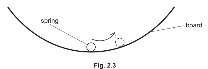
• Release the spring. The spring will roll from side to side on the board.
• Take measurements to determine the period $T$ of these oscillations.

$T$ = ______ $\text{s}$

2M Similar

DifficultyMedium-Easy

Worked solution

Working

Time $n = 20$ oscillations: $t = 33.0\ \text{s}$ .

T = \frac{t}{n} = \frac{33.0}{20} = 1.65\ \text{s}

Answer

$T = 1.65\ \text{s}$

Final answer

T = 1.65 s (example)

Detailed explanation

Background Concept

The period (T) is the time for one complete oscillation (one full back-and-forth cycle). Because reaction time is large compared with a single period, a better method is to time (n) oscillations and divide:

T = \frac{t}{n}

Repeating and averaging reduces random uncertainty.

Understanding the Question

With the spring rolling side-to-side on the curved board, you must take measurements to determine the period (T) and record it in seconds.

Approach

Choose a clear definition of one oscillation (e.g. centre (\rightarrow) one side (\rightarrow) back to centre (\rightarrow) the other side (\rightarrow) back to centre, or more simply “from one extreme back to the same extreme”).
Time a large number (n) of oscillations (e.g. 10–20) to reduce percentage timing uncertainty.
Divide total time (t) by (n) to obtain (T). Repeat and average.

Step-by-Step Reasoning

c-timing

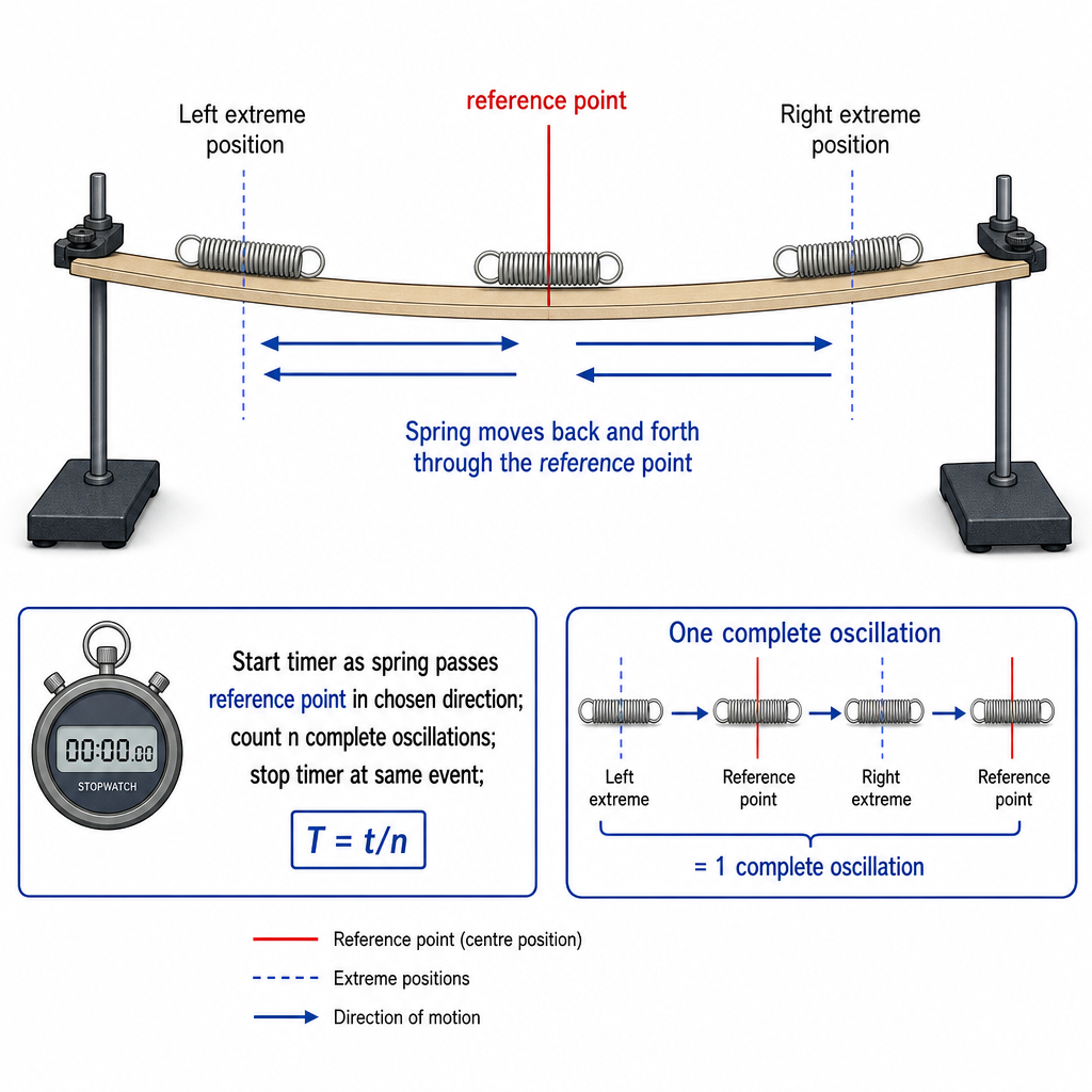
Displace the spring by a small distance and release.
Pick a reference point (often the centre position) and start timing as the spring passes that point in a chosen direction.
Count (n) complete oscillations using the same reference event each time (e.g. the (n)th time it passes the reference point in the same direction).
Stop the stopwatch at the end of the (n)th oscillation. Record (t).
Calculate (T = t/n). For example, (t=33.0\ \text{s}) for (n=20) gives (T=1.65\ \text{s}).
Repeat and take a mean (T).

Key Takeaways

Timing many oscillations reduces the effect of reaction time.
Use a consistent definition of “one oscillation”.

Common Mistakes

Timing only one oscillation (very large percentage uncertainty).
Miscounting oscillations.
Starting/stopping at different points in the motion each time.

Things to Be Careful About

Keep the displacement small and similar each time if possible.
Ensure the spring rolls smoothly without slipping.
Record (T) to a sensible precision based on the stopwatch (e.g. (0.01\ \text{s}) resolution does not guarantee (\pm 0.01\ \text{s}) accuracy due to reaction time).

Techniques used

time multiple oscillations and divide to obtain the periodrepeat timings and calculate a mean valueuse a consistent reference point to define one complete oscillation

(d)

• Adjust the apparatus until $d$ is in the range $66\text{ cm}$ to $74\text{ cm}$ . Ensure that the board does not touch the bench.
• Measure and record $d$ .

$d$ = ______ $\text{cm}$

• Repeat (c).

$T$ = ______ $\text{s}$

3M Similar

DifficultyMedium-Easy

Worked solution

Answer

(Example readings)

$d = 70.0\ \text{cm}$

Time $n = 20$ oscillations: $t = 28.0\ \text{s}$ .

T = \frac{t}{n} = \frac{28.0}{20} = 1.40\ \text{s}

$T = 1.40\ \text{s}$

Final answer

d = 70.0 cm, T = 1.40 s (example)

Detailed explanation

Background Concept

When investigating how one quantity depends on another, you change the independent variable (here (d)) and measure the dependent variable (here (T)). You must keep other factors as constant as possible and follow any constraints (e.g. board not touching the bench).

Understanding the Question

You must reset the apparatus so that (d) is between (66\ \text{cm}) and (74\ \text{cm}), ensuring the board does not touch the bench. Then measure and record (d), and repeat the period measurement from part (c).

Approach

Adjust stand spacing to the required range and check clearance from the bench.
Measure (d) as before (inside edges).
Measure (T) using the same timing method as in (c) (time many oscillations, divide by (n), repeat).

Step-by-Step Reasoning

Move the stands closer together until (66\le d \le 74\ \text{cm}).
Visually check the curved board does not touch the bench (contact would change the shape and introduce extra friction).
Measure (d) and record with units.
Time (n) oscillations and compute (T=t/n), repeating and averaging.

Key Takeaways

Only change (d); keep the timing method and other conditions consistent.
The “board does not touch the bench” instruction is important for validity.

Common Mistakes

Forgetting to ensure the board is clear of the bench.
Measuring a different definition of (d) than in (b).
Changing the timing method between runs (hurts comparison).

Things to Be Careful About

Ensure both clamp rods remain at the same height when you adjust (d).
Keep the spring displacement similar to part (c) so comparisons are meaningful.
Record both (d) and (T) with appropriate precision.

Techniques used

adjust the independent variable to lie within a specified rangemeasure the separation between reference points consistentlydetermine the period by timing multiple oscillations and dividing

(e)

It is suggested that the relationship between $T$ and $d$ is

(T - a) = kd

where $a$ is $0.70\text{ s}$ and $k$ is a constant.

(i)

Using your data, calculate two values of $k$ .

first value of $k$ = ______
second value of $k$ = ______

1M Similar

DifficultyMedium-Easy

Worked solution

Working

From

(T-a)=kd

k = \frac{T-a}{d}

Using $a = 0.70\ \text{s}$ :

First set: $T=1.65\ \text{s}$ , $d=95.0\ \text{cm}$

k_1 = \frac{1.65-0.70}{95.0} = \frac{0.95}{95.0} = 1.00\times 10^{-2}\ \text{s cm}^{-1}

Second set: $T=1.40\ \text{s}$ , $d=70.0\ \text{cm}$

k_2 = \frac{1.40-0.70}{70.0} = \frac{0.70}{70.0} = 1.00\times 10^{-2}\ \text{s cm}^{-1}

Answer

First value of $k = 1.0\times 10^{-2}\ \text{s cm}^{-1}$

Second value of $k = 1.0\times 10^{-2}\ \text{s cm}^{-1}$

Final answer

k1 = 1.0×10^-2 s cm^-1, k2 = 1.0×10^-2 s cm^-1 (example)

Detailed explanation

Background Concept

If a relationship is

(T-a)=kd

then (k) is the constant of proportionality between ((T-a)) and (d). To find (k) from one pair of readings, rearrange to

k = \frac{T-a}{d}

The unit of (k) comes from (\text{s}/\text{cm} = \text{s cm}^{-1}) when (d) is in cm.

Understanding the Question

You have two sets of measurements (two different values of (d), each with a measured (T)). Using (a=0.70\ \text{s}), you must calculate two values of (k), one from each dataset.

Approach

Rearrange the equation for (k).
For each dataset, compute ((T-a)) first, then divide by (d).
Quote (k) with a unit.

Step-by-Step Reasoning

Start with ((T-a)=kd) and divide both sides by (d).
For dataset 1: calculate (T-a). With (T=1.65\ \text{s}) and (a=0.70\ \text{s}), (T-a=0.95\ \text{s}). Then divide by (95.0\ \text{cm}) to get (k_1).
For dataset 2: similarly, (T-a=1.40-0.70=0.70\ \text{s}) and divide by (70.0\ \text{cm}) to get (k_2).
If the relationship is correct and uncertainties are small enough, (k_1) and (k_2) should be similar.

Key Takeaways

Always rearrange first: (k) is a ratio ((T-a)/d).
Subtraction ((T-a)) should be done before division.

Common Mistakes

Using (k = (T+a)/d) instead of ((T-a)/d).
Forgetting the unit of (k).
Mixing units (e.g. using (d) in m while treating it as cm).

Things to Be Careful About

(a) is given as (0.70\ \text{s}): ensure (T) is also in seconds.
If using (d) in cm, keep (k) in (\text{s cm}^{-1}). If you convert (d) to m, then (k) becomes (\text{s m}^{-1}).
After subtraction, significant figures can be limited by the least precise value involved.

Techniques used

rearrange an equation to solve for an unknown constantsubstitute experimental measurements into the relationshipcalculate two values and compare them for consistency

(ii)

Justify the number of significant figures that you have given for your values of $k$ .

1M Similar

DifficultyMedium-Easy

Worked solution

Answer

$k$ is found from $k = (T-a)/d$ .

The value of $(T-a)$ is limited by the precision of $T$ and $a$ (with $a = 0.70\ \text{s}$ given to 2 s.f.), so $(T-a)$ should be quoted to about 2 s.f.

Therefore $k$ should be given to 2 s.f. (matching the least precise quantity), e.g. $k = 1.0\times 10^{-2}\ \text{s cm}^{-1}$ .

Final answer

k to 2 s.f. (limited by T−a, with a = 0.70 s)

Detailed explanation

Background Concept

Significant figures in a calculated result should reflect the precision of the input data. For multiplication/division, the result should usually have the same number of significant figures as the least precise factor. For addition/subtraction, the limiting factor is often the number of decimal places (or the uncertainty) because subtraction can reduce the number of meaningful significant figures.

Understanding the Question

You calculated (k) from (k=(T-a)/d). You must justify how many significant figures you used when writing (k). The examiner expects you to link this to the precision of the measurements and to the given value (a=0.70\ \text{s}).

Approach

Identify which measured/given values limit the precision in (k).
Note that ((T-a)) involves subtraction, so its precision is limited by the precision of (T) and (a).
Apply the significant figure rule to the final division by (d).

Step-by-Step Reasoning

Suppose (T) is measured with a stopwatch and recorded to 2 d.p. (e.g. (1.65\ \text{s})). The given (a=0.70\ \text{s}) is to 2 d.p. and 2 s.f.
When calculating (T-a), the result cannot be more precise than the least precise decimal place in (T) and (a). So ((T-a)) is typically only reliable to about 2 d.p., and often only about 2 significant figures.
Then (k = (T-a)/d): the division means (k) should not have more significant figures than the least precise of ((T-a)) and (d). With ((T-a)) about 2 s.f., quoting (k) to 2 s.f. is appropriate.

Key Takeaways

Subtraction can reduce meaningful significant figures.
The final (k) should not be more precise than the least precise input.

Common Mistakes

Quoting (k) to 3–4 s.f. when (a) is only given to 2 s.f.
Confusing decimal places with significant figures.

Things to Be Careful About

Even if (d) is recorded as (95.0\ \text{cm}) (3 s.f.), ((T-a)) may still be the limiting value.
If your stopwatch readings are only to (0.1\ \text{s}), then (k) should be even fewer s.f.
Always include the unit with (k) and ensure the unit matches how you measured (d).

Techniques used

identify the least precise measurement affecting a calculated quantityapply significant-figure rules to derived resultsjustify rounding using instrument resolution and subtraction effects

(f)

It is suggested that the percentage uncertainty in the values of $k$ is $10\%$ .
Using this uncertainty, explain whether your results support the relationship in (e).

1M Similar

DifficultyMedium-Easy

Worked solution

Working

Using $k_1 = 1.0\times 10^{-2}$ and $k_2 = 1.0\times 10^{-2}\ \text{s cm}^{-1}$ ,

\%\ \text{difference} = \frac{|k_1-k_2|}{\frac{1}{2}(k_1+k_2)}\times 100 = 0\%

Since $0\% < 10\%$ , the two values agree within the stated uncertainty.

Answer

Yes, the results support the relationship in (e).

Final answer

Yes, supports (k values agree within 10%).

Detailed explanation

Background Concept

To test whether results support a suggested relationship, you check whether repeated/independent determinations of a constant agree within experimental uncertainty. If the uncertainty in (k) is (10%), then values that differ by less than about (10%) are considered consistent.

Understanding the Question

You are told: “percentage uncertainty in the values of (k) is (10%).” Using this, you must decide whether your two calculated (k) values support ((T-a)=kd).

Approach

Compute how different the two (k) values are (percentage difference).
Compare that difference with (10%).
Conclude whether they agree within uncertainty.

Step-by-Step Reasoning

A convenient comparison is the percentage difference:

\%\ \text{difference} = \frac{|k_1-k_2|}{\text{mean of }k_1\text{ and }k_2}\times 100

If this percentage difference is (\le 10%), then the values are consistent with the proposed relationship.
If it is (\gg 10%), then either the relationship is not supported or the experiment has unaccounted systematic errors.

Key Takeaways

“Support the relationship” means “results are consistent within uncertainty”, not “exactly equal”.

Common Mistakes

Comparing raw difference (|k_1-k_2|) without converting to a percentage.
Using (10%) uncertainty on (d) or (T) instead of on (k), when the question explicitly states it is for (k).

Things to Be Careful About

Use a clear numerical comparison (percentage difference or overlap of (\pm 10%) ranges around each (k)).
State the conclusion explicitly: “agree within 10% therefore supports” (or “do not agree, therefore does not support”).

Techniques used

compare two calculated values using a stated percentage uncertaintycalculate a percentage differencedraw a consistency conclusion based on overlap within uncertainty

(g)

(i)

Describe four sources of uncertainty or limitations of the procedure for this experiment.
For any uncertainties in measurement that you describe, you should state the quantity being measured and a reason for the uncertainty.

4M Similar

DifficultyMedium

Worked solution

Answer

Uncertainty in timing (measuring $t$ and hence $T$ ): reaction time when starting/stopping the stopwatch.
Difficulty defining one oscillation (affects $t$ and $T$ ): spring does not pass exactly the same point each time / extremes not sharp.
Motion not perfectly repeatable (affects $T$ ): amplitude changes due to energy loss (friction), so period may change during timing.
Apparatus alignment/geometry (affects $d$ and shape of board): clamp rods may not be exactly the same height or board may twist, changing curvature and hence $T$ for the same $d$ .

Final answer

Four valid uncertainties/limitations listed (see solution).

Detailed explanation

Background Concept

In evaluation, you gain marks by naming specific limitations and linking them to what they affect (e.g. (d) or (T)) and why they introduce uncertainty. Good answers distinguish timing uncertainties (often random) from systematic effects (e.g. geometry changing the curvature).

Understanding the Question

You must describe four sources of uncertainty or limitations in the procedure. If you mention measurement uncertainty, you must name the quantity measured and the reason for the uncertainty.

Approach

Think through each measured quantity and each physical process:

Measuring (d): reading a ruler; defining the inside edges; alignment.
Measuring (T): deciding what counts as one oscillation; human reaction time.
The oscillation itself: friction, slipping, changing amplitude, non-uniform curvature.
Pick four distinct points and explain each.

Step-by-Step Reasoning

Examples of creditworthy points (any four, well explained):

Timing uncertainty in (t) (and hence (T)): human reaction time starting/stopping stopwatch is comparable to tenths of a second.
Counting/definition of oscillation ((T)): the spring’s turning points may not be sharp; it may not reach identical extremes, making it hard to count complete cycles consistently.
Energy loss/friction ((T)): rolling friction and possible slipping cause amplitude to decay; dynamics may change during the timed interval, affecting the measured average period.
Curvature not exactly reproducible ((T) at fixed (d)): if clamp rods are not the same height or the board twists, the shape of the “track” changes even when (d) is the same.
Uncertainty in (d): inside edges may be hard to define; ruler alignment may not be exactly parallel to the stand separation; parallax when reading.
Spring not constrained to one line: spring may drift sideways, giving a slightly different path length/curvature each cycle.

Key Takeaways

State the quantity ((d), (t), (T)) and the reason.
Limitations often relate to timing, alignment, and non-ideal motion.

Common Mistakes

Writing vague statements like “human error” without specifying the quantity or mechanism.
Repeating the same idea in different words (e.g. “reaction time” and “starting stopwatch late”).
Giving an improvement instead of a limitation.

Things to Be Careful About

Ensure your four points are distinct.
For measurement uncertainties, always include both: the quantity and why it’s uncertain.
Include at least one limitation that affects the physics of the motion (not just reading instruments), because this experiment’s behaviour depends strongly on the board shape.

Techniques used

identify random and systematic sources of uncertaintylink each uncertainty to a specific measured quantitystate a physical reason for each limitation

(ii)

Describe four improvements that could be made to this experiment. You may suggest the use of other apparatus or different procedures.

4M Similar

DifficultyMedium

Worked solution

Answer

Measure $T$ using video analysis / motion sensor (or light gate with a flag) to remove reaction time.
Time a larger number of oscillations and repeat several times, then take a mean $T$ .
Add a fixed fiducial marker at the centre and define one oscillation as successive passes in the same direction to reduce counting ambiguity.
Use a spirit level / set square and a fixed height gauge to ensure both clamp rods are exactly the same height and the board is not twisted.

Final answer

Four valid improvements listed (see solution).

Detailed explanation

Background Concept

Improvements should directly reduce uncertainties or control variables better. The best answers explicitly connect: “This improvement reduces this limitation because …”. Common themes: reduce timing uncertainty, improve repeatability, control alignment/geometry, and stabilise the motion.

Understanding the Question

You must propose four improvements to the experiment. You may suggest extra apparatus or changed procedures.

Approach

Start from typical limitations:

Reaction time and ambiguous cycle counting (\rightarrow) use automated timing and a fiducial marker.
Poor repeatability (\rightarrow) more oscillations, repeated runs, averaging.
Geometry not controlled (\rightarrow) better alignment tools, fixed jigs.
Provide four distinct improvements.

Step-by-Step Reasoning

Examples of creditworthy improvements (any four, clearly described):

Automated timing: use video analysis (frame-by-frame) or a motion sensor/data logger to obtain (T) without human reaction time.
Increase timing interval: time (n\ge 20) oscillations and divide by (n); repeat at least 3 times and average (T) to reduce random scatter.
Better definition of oscillation: add a high-contrast centre marker; time successive crossings in the same direction so each cycle is defined consistently.
Improve alignment/shape control: use a spirit level and a height gauge to set both clamp rods to identical heights; ensure the board is not twisted, improving reproducibility for a given (d).
Reduce unwanted motion: add side guides to keep the spring moving in one line (without significant friction), reducing sideways drift.
Surface consistency: ensure the board surface is clean/dry and the spring is consistent between runs to reduce variation due to changing friction.

Key Takeaways

Improvements must be practical and must target specific uncertainties.
Averaging and automation are strong, commonly accepted improvements.

Common Mistakes

Giving the same improvement four times (e.g. “repeat readings” in different wording).
Suggesting unrealistic equipment without explaining how it would be used.
Improvements that do not connect to the actual limitation (e.g. “use a micrometer” for measuring (d) of ~1 m).

Things to Be Careful About

Ensure each improvement is distinct.
Where possible, explicitly say what quantity’s uncertainty is reduced ((T), (d), or board shape).
Keep suggested changes consistent with the experiment (the spring must still be able to roll freely).

Techniques used

propose method changes that reduce specific uncertaintiesmatch each improvement to a corresponding limitationsuggest appropriate additional apparatus for better measurement