Physics 9702/34 — May/June 2024

Cambridge AS Level · Advanced Practical Skills · worked solutions for every part, with the mark scheme

questions

marks

120

minutes

Topics Manipulation, Measurement and Observation · Presentation of Data and Observations · Analysis, Conclusions and Evaluation

Q1MediumManipulation, Measurement and ObservationPresentation of Data and ObservationsAnalysis, Conclusions and Evaluation

In this experiment, you will investigate the equilibrium position of a pulley system.

(a)

● Assemble the apparatus as shown in Fig. 1.1 with the rods of the stands approximately $50\text{ cm}$ apart.

Fig. 1.1

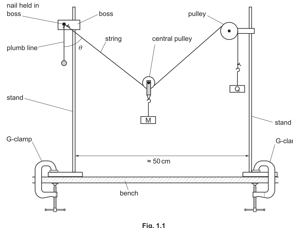
● Adjust the pulley fixed to the stand so that the top of the pulley is approximately $60\text{ cm}$ above the bench.
● Adjust the boss holding the nail so that the nail is approximately $60\text{ cm}$ above the bench.
● Use some of the slotted masses to add a mass of $70\text{ g}$ to Q.
● The mass added to Q is $x$ . Record the value of $x$ .

$x$ = ______ $\text{g}$

● The angle between the plumb line and the string is $\theta$ , as shown in Fig. 1.1.
Measure and record $\theta$ .

$\theta$ = ______ $^{\circ}$

● Carefully remove the slotted masses from Q.

1M Similar

DifficultyEasy

Worked solution

Answer

$x = 70\ \text{g}$

$\theta = 34^\circ$ (example reading, measured with a protractor)

Final answer

x = 70 g, θ = student-dependent

Detailed explanation

Background Concept

This is an equilibrium practical: the pulley system settles so the forces at the nail balance. The experiment uses measurements (mass added and angle) to test a proposed linear relationship.

The quantities to record here are:

$x$ : the added slotted mass on $Q$ (a direct mass reading in $\text{g}$ )
$\theta$ : the angle between the plumb line (true vertical) and the string at the nail (measured in degrees).

Understanding the Question

You are told exactly how to set the apparatus geometry (stands about $50\ \text{cm}$ apart, pulley/nail about $60\ \text{cm}$ above the bench). Then you add $70\ \text{g}$ to $Q$ , define this added mass as $x$ , and measure the angle $\theta$ shown at the nail.

Finally you remove the slotted masses (so you can then vary $x$ later in part (b)).

Approach

Set up the equipment to the stated dimensions so the geometry is consistent.
Add slotted masses totaling $70\ \text{g}$ to $Q$ and record $x$ with unit.
Measure $\theta$ using a protractor positioned at the nail, using the plumb line as the vertical reference.

Step-by-Step Reasoning

Add slotted masses until the total added mass is $70\ \text{g}$ . Record: $x = 70\ \text{g}$ .
Allow the system to come to rest.
Measure the angle between:
- the plumb line (vertical), and
- the string leaving the nail.
  Record $\theta$ to the nearest degree (typical for a protractor), e.g. $\theta = 34^\circ$ .
Remove the added slotted masses so you can start varying $x$ from a known baseline.

Key Takeaways

Record masses with correct units.
Measure the specified angle at the correct location and with the correct reference line (plumb line = vertical).

Common Mistakes

Measuring $\theta$ from the horizontal instead of from the plumb line.
Reading the wrong protractor scale (inner vs outer scale).
Recording $x$ without units or recording the total mass of $Q$ instead of the added mass $x$ .

Things to Be Careful About

Let the system settle before reading $\theta$ (avoid oscillations).
Place the protractor so its centre is at the nail to avoid systematic error.
Avoid parallax when reading the protractor scale.

Techniques used

assemble apparatus to specified geometrymeasure an angle with a protractor at the point of interestrecord measured quantities with appropriate units and precision

(b)

By using different numbers of slotted masses, vary $x$ . For each value of $x$ , measure $\theta$ .

Repeat until you have six sets of values of $x$ and $\theta$ .

Record your results in a table. Include values of $\frac{1}{\cos \theta}$ in your table.

10M Similar

DifficultyMedium

Worked solution

Answer

Record six sets of values of $x$ and $\theta$ and calculate $\dfrac{1}{\cos\theta}$ .

Example of a suitable table (values are illustrative):

$x\ /\ \text{g}$	$\theta\ /\ ^\circ$	$1/\cos\theta$
20	34	1.21
40	44	1.39
60	51	1.59
80	56	1.79
100	60	2.00
120	63	2.20

Final answer

Six readings in a table of x, θ and 1/cosθ (student-dependent values).

Detailed explanation

Background Concept

In Paper 3 you must collect enough data to reveal a trend and then process it to test a suggested relationship. When an equation involves a function such as $\cos\theta$ , it is common to calculate a derived quantity (here $1/\cos\theta$ ) so that a straight-line graph can be drawn later.

Good tables:

have clear headings with quantity and unit,
contain all raw data and calculated data together,
use consistent precision (decimal places) down each column.

Understanding the Question

You must:

vary the added mass $x$ by changing the number of slotted masses,
measure the corresponding angle $\theta$ each time,
obtain six pairs $(x,\theta)$ ,
and include a calculated column for $1/\cos\theta$ .

Approach

Choose at least six different values of $x$ spread over a sensible range (not all close together).
For each $x$ , wait for equilibrium and measure $\theta$ .
Compute $1/\cos\theta$ for each reading (calculator in degree mode).
Present all results in one table with headings and consistent rounding.

Step-by-Step Reasoning

Independent variable: $x$ (added mass in $\text{g}$ ). Choose values such as $20\ \text{g}$ to $120\ \text{g}$ in equal steps if possible.
Dependent variable: $\theta$ , read to nearest degree.
For each row:
1. Record $x$ .
2. Measure $\theta$ .
3. Calculate $\cos\theta$ (calculator in degrees), then calculate $1/\cos\theta$ .
Round $1/\cos\theta$ sensibly (typically 2 or 3 s.f. is adequate because $\theta$ is only to $1^\circ$ ).

Key Takeaways

Collect enough data points (six) and ensure a good spread in $x$ .
Include both measured ( $x$ , $\theta$ ) and derived ( $1/\cos\theta$ ) quantities in one clear table.

Common Mistakes

Fewer than six sets of readings.
Narrow range of $x$ (gives a poor graph and unreliable gradient).
Calculator set to radians instead of degrees.
Missing units in headings (e.g. writing just $x$ instead of $x/\text{g}$ ).

Things to Be Careful About

Ensure the system is stationary before reading $\theta$ .
Use consistent decimal places for $1/\cos\theta$ down the column.
If repeat readings are taken, record them properly (or average them) rather than overwriting values.

Techniques used

vary the independent variable over a suitable rangerecord repeated readings systematically in a single tablecalculate a derived quantity from measured valuesuse consistent significant figures and decimal places within columns

(c)

(i)

Plot a graph of $\frac{1}{\cos \theta}$ on the $y$ -axis against $x$ on the $x$ -axis.

3M Similar

DifficultyMedium-Easy

Worked solution

Answer

Plot $y = \dfrac{1}{\cos\theta}$ (no unit) on the $y$ -axis against $x/\text{g}$ on the $x$ -axis.

Use a suitable scale (at least half the grid in each direction).
Plot all six points accurately.

Final answer

Graph of 1/cosθ (y) against x (x-axis).

Detailed explanation

Background Concept

A straight-line graph is used to test linear relationships of the form $y = mx + c$ . To obtain a reliable gradient and intercept:

axes must be clearly labelled,
scales must be sensible (not cramped or awkward),
points must be plotted accurately.

Understanding the Question

You have already calculated $1/\cos\theta$ for each measured $\theta$ . Now you must plot a graph with:

horizontal axis: $x$ ,
vertical axis: $1/\cos\theta$ .

Approach

Decide the range of $x$ and $1/\cos\theta$ from your table.
Choose scales so the plotted area uses most of the available grid.
Label axes with the correct quantities and units.
Plot each point as a small cross.

Step-by-Step Reasoning

diagram-c-i-graph-layout

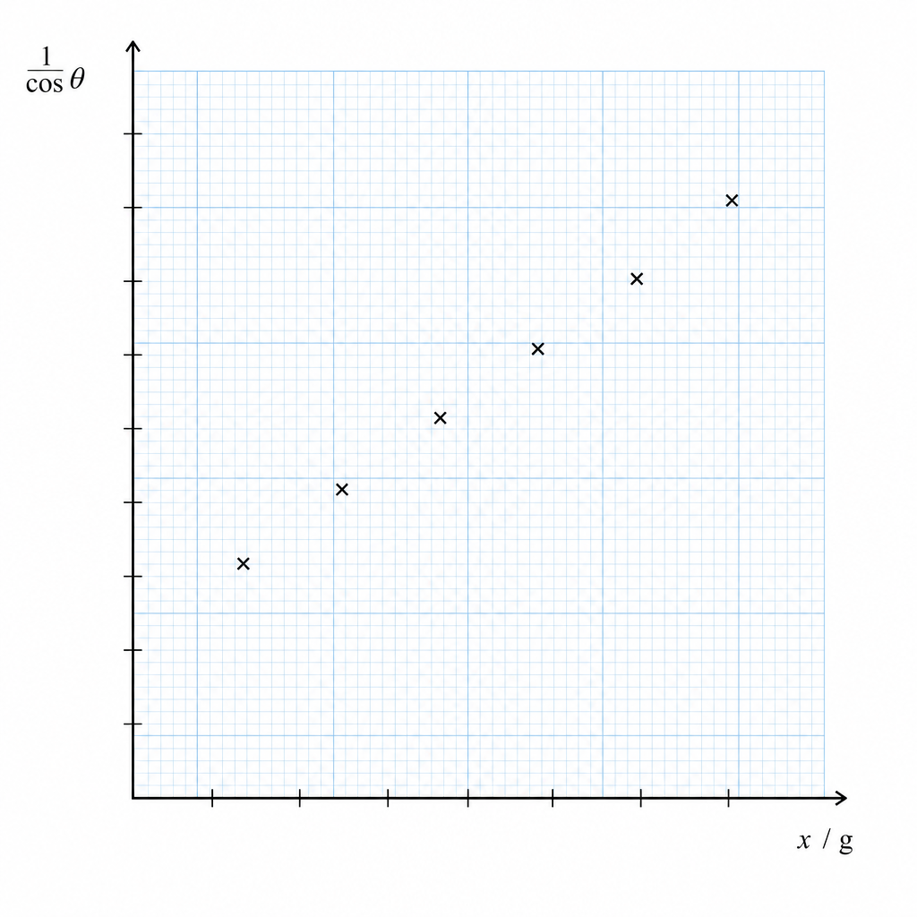
$x$ is in $\text{g}$ , so label the axis as $x/\text{g}$ .
$1/\cos\theta$ is dimensionless (a ratio), so label as $1/\cos\theta$ (no unit).
Choose a scale such as 20 g per large square (example only) if it fits your data range well.
Plot each pair $(x, 1/\cos\theta)$ using a sharp pencil and ruler for reading.

Key Takeaways

Correct axis labels: quantity and unit.
Good scale choice improves accuracy of gradient and intercept.

Common Mistakes

Swapping axes (plotting $x$ on $y$ -axis).
Writing units incorrectly (e.g. putting degrees on $1/\cos\theta$ ).
Using a tiny portion of the grid (reduces precision).

Things to Be Careful About

Do not force the graph through the origin unless the data clearly supports it.
Plotting should reflect your table values; do not “smooth” points before drawing the best-fit line in part (ii).

Techniques used

choose appropriate axes and scales to use most of the gridplot measured/calculated points with correct orientationlabel axes with quantity and unit

(ii)

Draw the straight line of best fit.

1M Similar

(iii)

Determine the gradient and $y$ -intercept of this line.

gradient = ______
$y$ -intercept = ______

2M Similar

DifficultyMedium

Worked solution

Working

Choose two points on the best-fit line well separated:

\text{gradient} = \frac{\Delta y}{\Delta x} = \frac{(1/\cos\theta)_2 - (1/\cos\theta)_1}{x_2 - x_1}

Read the $y$ -intercept at $x = 0$ from the line.

(Example from a typical straight line: gradient $\approx 1.0 \times 10^{-2}\ \text{g}^{-1}$ , $y$ -intercept $\approx 1.0$ .)

Answer

gradient $= 1.0 \times 10^{-2}\ \text{g}^{-1}$ (example)

$y$ -intercept $= 1.0$ (example)

Final answer

Gradient and y-intercept from graph (student-dependent).

Detailed explanation

Background Concept

For a straight-line graph,

y = mx + c

the gradient is $m = \Delta y/\Delta x$ ,
the $y$ -intercept is $c$ (the value of $y$ when $x=0$ ).

Using a large triangle on the best-fit line reduces the fractional uncertainty in $\Delta x$ and $\Delta y$ .

Understanding the Question

You must use your best-fit line from (c)(ii) to find:

the gradient of the line,
the $y$ -intercept of the line.

These will be used later to identify constants in the suggested relationship.

Approach

Select two points on the drawn best-fit line that are far apart (not necessarily actual data points).
Read their coordinates carefully.
Compute gradient $= \Delta y / \Delta x$ .
Read the intercept where the line crosses the $y$ -axis.

Step-by-Step Reasoning

diagram-c-iii-gradient-triangle

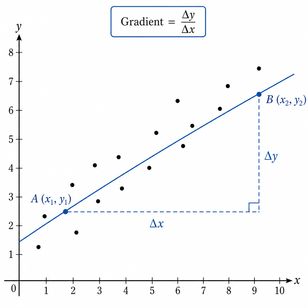
Pick two points on the line, e.g. near the left and right ends of the plotted region.
Suppose the points are $(x_1, y_1)$ and $(x_2, y_2)$ .
Compute changes:

\Delta x = x_2 - x_1, \qquad \Delta y = y_2 - y_1

Then the gradient is:

\text{gradient} = \frac{\Delta y}{\Delta x}

Units: $y$ is dimensionless, $x$ is in $\text{g}$ , so gradient has unit $\text{g}^{-1}$ .

The $y$ -intercept is read at the point where the line crosses the vertical axis ( $x=0$ ). This intercept is dimensionless.

Key Takeaways

Gradient is always $\Delta y/\Delta x$ (not the other way around).
Use points on the best-fit line, widely spaced, to improve accuracy.

Common Mistakes

Using two adjacent grid squares (small triangle), giving a very imprecise gradient.
Calculating $\Delta x/\Delta y$ by mistake.
Taking coordinates from raw data points that do not lie on the best-fit line.

Things to Be Careful About

Read the correct scales from each axis.
Keep enough significant figures during the gradient calculation, then round sensibly.
Quote the intercept value consistent with your graph-reading precision.

Techniques used

calculate gradient from two well-separated points on the best-fit linedetermine y-intercept by reading where the line crosses the y-axisuse a large triangle to reduce percentage reading error

(d)

It is suggested that the quantities $\theta$ and $x$ are related by the equation

\frac{1}{\cos \theta} = ax + b

where $a$ and $b$ are constants.

Use your answers in (c)(iii) to determine the values of $a$ and $b$ . Give appropriate units.

$a$ = ______
$b$ = ______

2M Similar

DifficultyMedium-Easy

Worked solution

Working

Given

\frac{1}{\cos\theta} = ax + b

Comparing with $y = mx + c$ for a graph of $y = \dfrac{1}{\cos\theta}$ against $x$ :

a = \text{gradient}, \qquad b = y\text{-intercept}

Units: $\dfrac{1}{\cos\theta}$ is dimensionless, so $b$ has no unit and $a$ has unit $\text{g}^{-1}$ (since $x$ is in $\text{g}$ ).

Answer

$a =$ gradient $\ (\text{g}^{-1})$

$b =$ $y$ -intercept (no unit)

Final answer

a = gradient (g^-1), b = y-intercept (dimensionless)

Detailed explanation

Background Concept

When you plot a graph in the form $y$ against $x$ , a linear relationship has the form:

y = mx + c

The gradient $m$ and intercept $c$ can be interpreted as constants in the physical equation.

Understanding the Question

You are told the suggested model is:

\frac{1}{\cos\theta} = ax + b

You have already plotted $\dfrac{1}{\cos\theta}$ (vertical axis) against $x$ (horizontal axis) and found the gradient and intercept. You must now identify $a$ and $b$ and state appropriate units.

Approach

Identify $y$ with $\dfrac{1}{\cos\theta}$ and $x$ with $x$ .
Compare directly to $y = mx + c$ .
Use units to check: $y$ is dimensionless, so $ax$ must be dimensionless.

Step-by-Step Reasoning

From the graph definition:
- gradient $m$ satisfies $m = \Delta y/\Delta x$ .
- intercept $c$ is $y$ when $x=0$ .
Comparing:

\frac{1}{\cos\theta} = ax + b \quad \leftrightarrow \quad y = mx + c

So:

a = m, \qquad b = c

Units:
- $\cos\theta$ is a ratio, so it has no unit, therefore $1/\cos\theta$ has no unit.
- Therefore $ax$ must be unitless, so $a$ must have units of $1/x$ .
- Since $x$ is measured in $\text{g}$ , $a$ has units $\text{g}^{-1}$ .
- $b$ has the same units as $y$ , i.e. no unit.

Key Takeaways

The constant multiplying $x$ is the gradient.
The constant added is the intercept.
Units come from ensuring each term has the same dimensions.

Common Mistakes

Giving $b$ a unit of degrees or grams.
Using $a = 1/\text{gradient}$ instead of $a = \text{gradient}$ .

Things to Be Careful About

Your value of $a$ depends on the unit used for $x$ . If you plotted $x$ in $\text{kg}$ instead of $\text{g}$ , the numerical value of $a$ would change accordingly.

Techniques used

match a straight-line graph to y = mx + cidentify constants from gradient and interceptassign units by comparing dimensions of both sides

(e)

The mass of M is $M$ and the mass of Q is $Q$ .

The constants $a$ and $b$ are related to $M$ and $Q$ by

a = \frac{2}{M} \text{ and } b = \frac{2Q}{M}

Calculate values for $M$ and $Q$ .

$M$ = ______ $\text{g}$
$Q$ = ______ $\text{g}$

1M Similar

DifficultyMedium-Easy

Worked solution

Working

Given

a = \frac{2}{M}

M = \frac{2}{a}

Also

b = \frac{2Q}{M} \;\Rightarrow\; Q = \frac{bM}{2}

Answer

M = \frac{2}{a}\ \text{g}

Q = \frac{bM}{2}\ \text{g}

Final answer

M = 2/a g, Q = (bM)/2 g (student-dependent).

Detailed explanation

Background Concept

Once you have experimental constants from a straight-line graph, you often use a theoretical model to link those constants to physical quantities. Here, the constants $a$ and $b$ are related to masses $M$ and $Q$ .

Algebra skills needed:

rearrange to make a variable the subject,
substitute carefully and keep track of units.

Understanding the Question

You are given:

a = \frac{2}{M} \quad \text{and} \quad b = \frac{2Q}{M}

You have already found $a$ and $b$ from the graph. You must calculate numerical values of the masses $M$ and $Q$ .

Approach

Rearrange $a = 2/M$ to find $M$ .
Substitute $M$ into $b = 2Q/M$ and rearrange to find $Q$ .
Use grams if your $a$ was in $\text{g}^{-1}$ .

Step-by-Step Reasoning

From

a = \frac{2}{M}

multiply both sides by $M$ and divide by $a$ :

M = \frac{2}{a}

Then use

b = \frac{2Q}{M}

Multiply both sides by $M$ :

bM = 2Q

So:

Q = \frac{bM}{2}

Unit check:

If $a$ is in $\text{g}^{-1}$ , then $2/a$ is in $\text{g}$ , so $M$ comes out in grams.
$b$ is dimensionless, so $Q$ has same unit as $M$ (grams).

Key Takeaways

Constants from graphs can be used to determine physical parameters.
Always match units: the unit chosen for $x$ determines the unit of $a$ and therefore the unit of $M$ .

Common Mistakes

Using $M = a/2$ instead of $M = 2/a$ .
Forgetting to divide by 2 when finding $Q$ .
Mixing $\text{kg}$ and $\text{g}$ (e.g. plotting $x$ in g but using $M$ in kg).

Things to Be Careful About

If your graph used $x$ in $\text{kg}$ , then $a$ would be in $\text{kg}^{-1}$ and $M$ would come out in $\text{kg}$ . Convert if the answer is required in $\text{g}$ .
Quote $M$ and $Q$ to a sensible number of significant figures consistent with the uncertainty in the gradient/intercept.

Techniques used

rearrange equations to make the required variable the subjectsubstitute experimental constants into derived formulaehandle units consistently between constants and masses

Q2MediumManipulation, Measurement and ObservationAnalysis, Conclusions and EvaluationPresentation of Data and Observations

In this experiment, you will investigate the effect of air resistance on a spinning card.

(a)

(i)

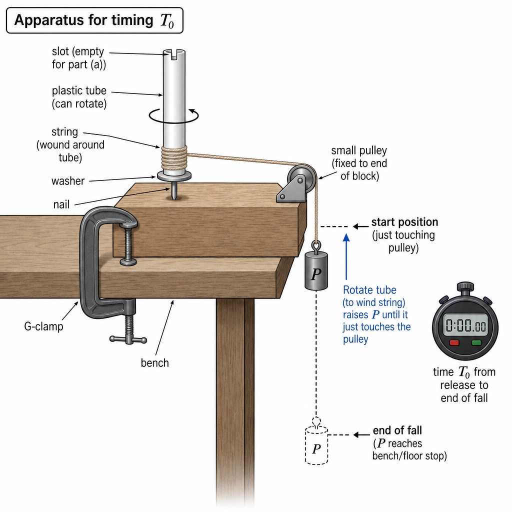
● Assemble the apparatus as shown in Fig. 2.1, with the washer and plastic tube over the nail.

Fig. 2.1

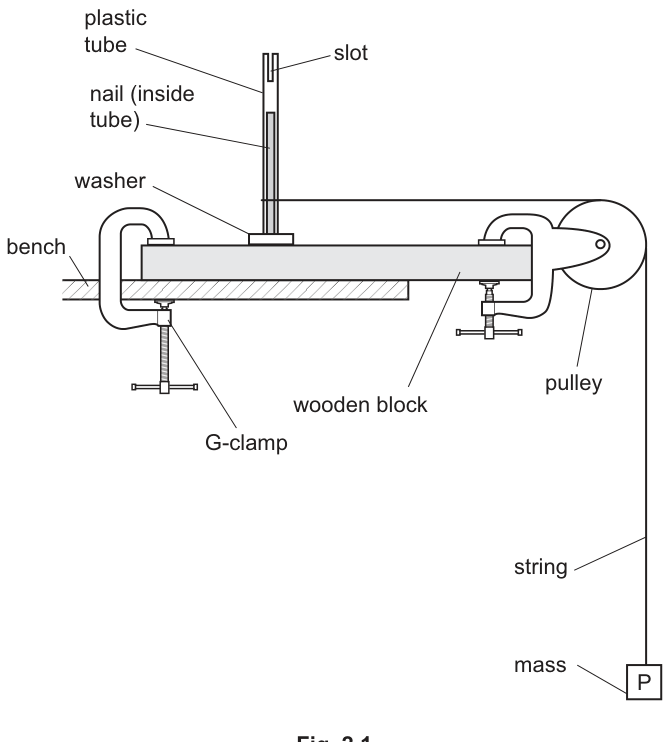
● Rotate the plastic tube so that P rises until it just touches the pulley.
● Release the plastic tube so that P falls.
● Measure and record the time $T_0$ for P to reach the end of its fall.

$T_0$ = ______

2M Similar

DifficultyMedium-Easy

Worked solution

Answer

(Example) $T_0 = 1.30\ \text{s}$

Final answer

T0 ≈ 1.30 s

Detailed explanation

Background Concept

Timing experiments usually involve measuring the time interval between two clearly defined events. The quality of a time measurement depends on (i) the resolution of the timer (e.g. $0.01\ \text{s}$ for a digital stopwatch) and (ii) human reaction time when starting/stopping. Repeating the measurement and taking a mean reduces random uncertainty.

Understanding the Question

You are asked to set up the apparatus (plastic tube on a nail, string over pulley, mass $P$ ) and measure the time $T_0$ for $P$ to fall from the release point (when the tube is released) to the end of its fall.

The key is to keep the start and end points consistent for every run.

setup-2ai

Approach

Assemble the apparatus as shown and check the string runs freely over the pulley.
Raise $P$ until it just touches the pulley (this defines a consistent start position).
Release the tube and time the motion of $P$ until it reaches the end of its fall (consistent end position).
Repeat and average to obtain $T_0$ .

Step-by-Step Reasoning

Set the tube so that $P$ just touches the pulley: this fixes the same initial height each time.
Start the stopwatch at the instant you release the tube (or as close as possible).
Stop the stopwatch when $P$ reaches the end of its fall (choose a clear end-point, e.g. when $P$ first hits the bench/floor stop).
Repeat at least 3 times.
Record the mean time as $T_0$ and include the unit seconds.

Example recording:

$T_0$ readings: $1.29\ \text{s},\ 1.31\ \text{s},\ 1.30\ \text{s}$
Mean $T_0 = 1.30\ \text{s}$

Key Takeaways

Define a clear start and end event before timing.
Repeats and averaging improve reliability.
Record with an appropriate unit and precision.

Common Mistakes

Timing from the wrong start point (e.g. from when $P$ starts moving rather than release moment), giving inconsistent $T_0$ .
Stopping the timer inconsistently (e.g. when $P$ is near the end rather than at a defined point).
Recording no unit or an over-precise value that doesn’t match the stopwatch/reaction-time limitation.

Things to Be Careful About

Ensure the string does not slip on the tube during the fall.
Make sure $P$ does not swing; swinging changes motion and makes the end-point hard to judge.
Keep the initial condition “just touches the pulley” the same each time.

Techniques used

assemble apparatus to match the diagram and ensure free motionuse a stopwatch to time an interval between two defined eventsrepeat timing measurements and take a mean valuerecord a time reading with an appropriate resolution and unit

(ii)

Estimate the percentage uncertainty in your value of $T_0$ . Show your working.

percentage uncertainty = ______ $\%$

1M Similar

DifficultyMedium-Easy

Worked solution

Working

(Example) stopwatch uncertainty $\Delta T_0 \approx \pm 0.20\ \text{s}$ .

\%\ \text{uncertainty} = \frac{\Delta T_0}{T_0}\times 100 = \frac{0.20}{1.30}\times 100 = 15\%.

Answer

$15\%$

Final answer

15%

Detailed explanation

Background Concept

The percentage uncertainty in a measured quantity $x$ is

\%\ \text{uncertainty} = \frac{\Delta x}{x}\times 100.

For time measurements with a hand-operated stopwatch, the dominant uncertainty is usually human reaction time, often estimated as about $\pm 0.2\ \text{s}$ for a single start/stop timing (some candidates use $\pm 0.1\ \text{s}$ ; the key is that the estimate must be reasonable and then used correctly).

Understanding the Question

You have measured $T_0$ (time for $P$ to fall with no card). You must estimate the percentage uncertainty in your measured $T_0$ and show working.

Approach

Decide an absolute uncertainty $\Delta T_0$ (from stopwatch resolution and/or reaction time).
Substitute into $\frac{\Delta T_0}{T_0}\times 100$ .

Step-by-Step Reasoning

Suppose $T_0 = 1.30\ \text{s}$ .
Take $\Delta T_0 = 0.20\ \text{s}$ (reaction-time dominated).

\%\ \text{uncertainty} = \frac{0.20}{1.30}\times 100 = 15.38\% \approx 15\%.

Rounding to about 2 significant figures is appropriate because the uncertainty estimate itself is approximate.

Key Takeaways

Use $\% = (\text{absolute}/\text{measured})\times 100$ .
For stopwatch timings, reaction time often dominates over the digital resolution.

Common Mistakes

Using $\frac{T_0}{\Delta T_0}$ instead of $\frac{\Delta T_0}{T_0}$ .
Forgetting to multiply by $100$ .
Claiming an unrealistically small uncertainty (e.g. $\pm 0.01\ \text{s}$ ) for a hand-timed event.

Things to Be Careful About

If you repeat and average, the random uncertainty in the mean can reduce, but reaction-time/systematic judgement of start/stop often still limits the accuracy. State clearly what uncertainty you are using.
Keep units consistent (seconds in both numerator and denominator).

Techniques used

estimate absolute uncertainty from instrument resolution and reaction timecalculate a percentage uncertainty using absolute uncertainty divided by measured valuepresent uncertainty to a sensible number of significant figures

(b)

(i)

Fig. 2.2 shows card A.

Fig. 2.2

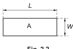
Measure and record the length $L$ and the width $W$ of the card, as shown in Fig. 2.2.

$L$ = ______
$W$ = ______

1M Similar

DifficultyEasy

Worked solution

Answer

(Example) $L = 12.0\ \text{cm}$

(Example) $W = 8.0\ \text{cm}$

Final answer

L ≈ 12.0 cm, W ≈ 8.0 cm

Detailed explanation

Background Concept

Measuring lengths accurately requires correct alignment of the object with the ruler scale, choosing appropriate reference points (edge to edge), and reading the scale without parallax error. The uncertainty is usually about $\pm 1\ \text{mm}$ for a typical ruler if used carefully.

Understanding the Question

You must measure the card’s length $L$ and width $W$ as indicated on the diagram. These will later be used in a calculation, so you should record them with a sensible precision (typically to the nearest $1\ \text{mm}$ or $0.1\ \text{cm}$ ) and include units.

Approach

Place the card so one edge aligns exactly with the ruler’s zero.
Measure to the opposite edge.
Repeat for the perpendicular dimension.
Record $L$ and $W$ to consistent precision.

Step-by-Step Reasoning

Align the long side of the card with the ruler and read the distance between the two edges to obtain $L$ .
Align the short side similarly to obtain $W$ .
Record values, e.g. $L = 12.0\ \text{cm}$ and $W = 8.0\ \text{cm}$ .

Key Takeaways

Correct alignment and avoiding parallax matter more than writing extra decimal places.
Always include units.

Common Mistakes

Not starting at the ruler zero (or using a damaged ruler end) without correcting for the offset.
Reading at an angle, producing parallax.
Recording inconsistent precision (e.g. $L=12\ \text{cm}$ but $W=8.03\ \text{cm}$ with no justification).

Things to Be Careful About

Measure the actual card edges (not including any rounded corners if present).
If the edges are not perfectly straight, measure at several points and use a best estimate.

Techniques used

use a ruler to measure linear dimensionsavoid parallax when reading a scalerecord lengths to an appropriate precision with units

(ii)

● Insert the card centrally into the slot at the top of the plastic tube with its length horizontal. If necessary, use a small piece of adhesive putty to fix it securely in the slot.
● Rotate the plastic tube so that P rises until it just touches the pulley.
● Release the plastic tube and measure the time $T$ for P to reach the end of its fall.

$T$ = ______

2M Similar

(c)

Repeat (b) using the card marked B.

$L$ = ______
$W$ = ______
$T$ = ______

3M Similar

DifficultyMedium-Easy

Worked solution

Answer

(Example) $L = 12.0\ \text{cm}$

(Example) $W = 4.0\ \text{cm}$

(Example) $T = 1.46\ \text{s}$

Final answer

Example: L ≈ 12.0 cm, W ≈ 4.0 cm, T ≈ 1.46 s

Detailed explanation

Background Concept

To investigate how air resistance depends on card dimensions, you repeat the procedure with a different card (B). Changing $L$ and/or $W$ changes the area interacting with air, which changes drag and therefore changes the time $T$ .

Understanding the Question

You must repeat part (b) for card B: measure $L$ and $W$ for card B and measure the corresponding fall time $T$ . The important idea is that everything else should stay the same so that differences in $T$ come from the card dimensions.

Approach

Measure $L$ and $W$ for B with the same method/precision as for A.
Insert card B centrally, same orientation (length horizontal).
Use the same start position for $P$ and same timing start/stop criteria.
Repeat timings and take a mean.

Step-by-Step Reasoning

Measure B’s dimensions and record them with units.
Time the fall several times; calculate the mean time.

Example record:

$L = 12.0\ \text{cm}$ , $W = 4.0\ \text{cm}$ , $T = 1.46\ \text{s}$ .

Key Takeaways

Consistency of method is crucial for comparing two sets of results.
Record all values with units and sensible precision.

Common Mistakes

Measuring card B with a different precision or unit without stating it.
Not keeping the same start height for $P$ , making comparison unreliable.

Things to Be Careful About

If card B is lighter/heavier and changes the rotational behaviour, note that as a possible limitation; ideally card thickness/material should be similar and only dimensions vary.
Ensure the card is securely fixed so it does not tilt during motion.

Techniques used

measure the dimensions of a second card using the same instrument and methodtime the fall for the second card under the same initial conditionsensure a fair test by keeping apparatus and procedure unchangedrecord results clearly with units and consistent precision

(d)

It is suggested that the relationship between $T$ , $T_0$ , $L$ and $W$ is

k(T - T_0) = L^2W

where $k$ is a constant.

(i)

Using your data, calculate two values of $k$ .

first value of $k$ = ______
second value of $k$ = ______

1M Similar

DifficultyMedium-Easy

Worked solution

Working

From

k(T-T_0)=L^2W

k=\frac{L^2W}{(T-T_0)}

(Example data) $T_0=1.30\ \text{s}$ .

Card A: $L=0.120\ \text{m}$ , $W=0.080\ \text{m}$ , $T=1.65\ \text{s}$

k=\frac{(0.120)^2(0.080)}{(1.65-1.30)}=3.3\times 10^{-3}\ \text{m}^3\ \text{s}^{-1}

Card B: $L=0.120\ \text{m}$ , $W=0.040\ \text{m}$ , $T=1.46\ \text{s}$

k=\frac{(0.120)^2(0.040)}{(1.46-1.30)}=3.6\times 10^{-3}\ \text{m}^3\ \text{s}^{-1}

Answer

first $k = 3.3\times 10^{-3}\ \text{m}^3\ \text{s}^{-1}$

second $k = 3.6\times 10^{-3}\ \text{m}^3\ \text{s}^{-1}$

Final answer

Example: k1 ≈ 3.3×10^-3 m^3 s^-1, k2 ≈ 3.6×10^-3 m^3 s^-1

Detailed explanation

Background Concept

When an experiment suggests a relationship such as

k(T-T_0)=L^2W,

$k$ should be constant for different cards if the relationship is correct. To test this, you calculate $k$ for each card using your measured $T$ , $T_0$ , $L$ , and $W$ .

Rearranging for $k$ gives

k=\frac{L^2W}{T-T_0}.

The units of $k$ depend on your chosen units for $L$ and $W$ . If you use metres, $L^2W$ has units $\text{m}^3$ , so $k$ has units $\text{m}^3\ \text{s}^{-1}$ .

Understanding the Question

You have two cards (A and B), so you have two sets of values for $L$ , $W$ , and $T$ (with one common $T_0$ ). You must compute two values of $k$ and later compare them.

Approach

For each card, compute $T-T_0$ first (this is the extra time due to the card).
Compute $L^2W$ .
Divide to find $k$ .
Keep units consistent (ideally convert cm to m before calculating).

Step-by-Step Reasoning

Using example values:

$T_0 = 1.30\ \text{s}$ .

Card A:

Convert: $L=12.0\ \text{cm}=0.120\ \text{m}$ , $W=8.0\ \text{cm}=0.080\ \text{m}$ .
Compute time difference: $T-T_0 = 1.65-1.30 = 0.35\ \text{s}$ .
Compute geometric factor:

L^2W = (0.120)^2(0.080) = 0.001152\ \text{m}^3.

Then

k = \frac{0.001152}{0.35} = 3.29\times 10^{-3}\ \text{m}^3\ \text{s}^{-1}.

Card B:

Convert: $L=0.120\ \text{m}$ , $W=4.0\ \text{cm}=0.040\ \text{m}$ .
$T-T_0 = 1.46-1.30 = 0.16\ \text{s}$ .
$L^2W = (0.120)^2(0.040) = 0.000576\ \text{m}^3$ .

k = \frac{0.000576}{0.16} = 3.60\times 10^{-3}\ \text{m}^3\ \text{s}^{-1}.

If the two $k$ values are similar (within experimental uncertainty), that supports the proposed relationship.

Key Takeaways

Rearranging to find a constant and calculating it for multiple trials is a standard way to test a model.
Converting to consistent units prevents hidden factor-of-10 errors.

Common Mistakes

Using $T$ instead of $T-T_0$ .
Squaring the wrong quantity (e.g. calculating $(LW)^2$ ).
Mixing cm and m in the same calculation.

Things to Be Careful About

If $T$ is very close to $T_0$ , then $T-T_0$ is small and its percentage uncertainty becomes large; this can make $k$ very uncertain.
Quote units for $k$ that match the units you used for $L$ and $W$ .

Techniques used

rearrange an equation to make a constant the subjectsubstitute measured values consistently (including units)calculate a derived quantity for two trialsuse consistent units for lengths and times

(ii)

Justify the number of significant figures that you have given for your values of $k$ .

1M Similar

DifficultyEasy

Worked solution

Answer

$k$ is calculated from measured values of $L$ , $W$ , $T$ and $T_0$ . The dominant uncertainty is in $(T-T_0)$ (stopwatch/reaction time), so $k$ is quoted to $2\ \text{s.f.}$ to match the least precise measurement / about $15\%$ uncertainty.

Final answer

k quoted to 2 s.f. (limited mainly by uncertainty in T − T0)

Detailed explanation

Background Concept

Significant figures in a calculated quantity should reflect the precision of the measured quantities used to calculate it. If one measurement has a large uncertainty, it limits the meaningful precision of the final result.

In this experiment, $k$ is found from

k=\frac{L^2W}{T-T_0}.

The value $T-T_0$ is often the limiting factor because it is a difference of two timings and can be relatively small, so its percentage uncertainty can be large.

Understanding the Question

You must explain why you chose the number of significant figures written for your calculated $k$ values.

Approach

Identify which measured value has the largest percentage uncertainty.
State that the calculated $k$ cannot be more precise than that.
Choose a sensible number of significant figures (often 2 or 3) consistent with the data.

Step-by-Step Reasoning

Typical ruler readings for $L$ and $W$ might be to $\pm 1\ \text{mm}$ , giving small percentage uncertainties (often a few percent).
Stopwatch timing with reaction time might have uncertainty around $\pm 0.2\ \text{s}$ . If $T-T_0$ is only, say, $0.16\ \text{s}$ to $0.35\ \text{s}$ , then the percentage uncertainty in $T-T_0$ can be large.
Therefore, quoting $k$ to many decimal places is not justified. With an uncertainty of order $15\%$ , quoting $k$ to $2\ \text{s.f.}$ is appropriate.

Key Takeaways

The least precise measurement (largest percentage uncertainty) sets the precision of the final derived result.
Differences like $T-T_0$ can have large fractional uncertainty.

Common Mistakes

Quoting $k$ to 4–5 significant figures because a calculator shows them.
Justifying significant figures by the number of decimal places instead of the actual uncertainty.

Things to Be Careful About

If your raw times are recorded to $0.01\ \text{s}$ , that does not automatically mean the uncertainty is $0.01\ \text{s}$ ; reaction time may dominate.
Be consistent: use the same significant figures for both values of $k$ unless there is a clear reason not to.

Techniques used

identify the least precisely known measured quantitymatch the significant figures of a derived quantity to the input data qualityjustify rounding using the size of experimental uncertainty

(e)

It is suggested that the percentage uncertainty in the values of $k$ is $15\%$ .

Using this uncertainty, explain whether your results support the relationship in (d).

1M Similar

DifficultyMedium-Easy

Worked solution

Working

(Example) $k_1 = 3.3\times 10^{-3}$ and $k_2 = 3.6\times 10^{-3}$ .

\%\ \text{difference} = \frac{|k_2-k_1|}{\left(\frac{k_1+k_2}{2}\right)}\times 100 = \frac{0.3\times 10^{-3}}{3.45\times 10^{-3}}\times 100 \approx 8.7\%.

Answer

Since $8.7\% < 15\%$ , the two values of $k$ agree within uncertainty, so the results support the relationship.

Final answer

Yes — k values agree within 15% uncertainty.

Detailed explanation

Background Concept

Experimental support for a proposed relationship often means that values of a supposed constant (here $k$ ) are consistent within the stated experimental uncertainty.

If each value of $k$ has a percentage uncertainty of $15\%$ , then two values are considered consistent if their difference is not more than what could be explained by these uncertainties. A common way to check is either:

compare the percentage difference between them to $15\%$ (a simple test), or
check whether the uncertainty ranges overlap (e.g. $k_1\pm 15\%$ overlaps $k_2\pm 15\%$ ).

Understanding the Question

You have calculated two values of $k$ from two different cards. You are told to assume the percentage uncertainty in $k$ is $15\%$ . You must use that to decide whether your results support the relationship $k(T-T_0)=L^2W$ .

Approach

Find how different the two $k$ values are (percentage difference).
Compare with $15\%$ .
State a conclusion (support / do not support) with a reason.

Step-by-Step Reasoning

Using example values:

$k_1 = 3.3\times 10^{-3}$
$k_2 = 3.6\times 10^{-3}$

Compute percentage difference (relative to the mean):

\%\ \text{difference} = \frac{|3.6-3.3|\times 10^{-3}}{\left(\frac{3.6+3.3}{2}\right)\times 10^{-3}}\times 100 = \frac{0.3}{3.45}\times 100 \approx 8.7\%.

Since $8.7\%$ is less than $15\%$ , the discrepancy is small enough to be explained by the experimental uncertainty, so the results are consistent with the model.

(Overlap method, also valid):

$k_1\pm 15\%$ gives a range from $0.85k_1$ to $1.15k_1$ .
$k_2\pm 15\%$ gives a range from $0.85k_2$ to $1.15k_2$ .
If these ranges overlap, the values are consistent.

Key Takeaways

“Supports the relationship” means agreement within the stated uncertainty, not exact equality.
Always justify the conclusion numerically.

Common Mistakes

Saying “they are different so it doesn’t work” without using the $15\%$ uncertainty.
Comparing using absolute difference only (e.g. $0.3\times 10^{-3}$ ) rather than percentage.

Things to Be Careful About

Use a clear comparison method and show the key step.
If your two $k$ values differ by more than $15\%$ , you should say results do not support the relationship (within this uncertainty) and briefly suggest why (e.g. timing uncertainty, friction changes).

Techniques used

apply a given percentage uncertainty to compare two measured constantscalculate a percentage difference between two valuesuse overlap of uncertainty ranges to assess consistency

(f)

(i)

Describe four sources of uncertainty or limitations of the procedure for this experiment.

For any uncertainties in measurement that you describe, you should state the quantity being measured and a reason for the uncertainty.

4M Similar

DifficultyMedium

Worked solution

Answer

Timing uncertainty in $T$ and $T_0$ due to human reaction time when starting/stopping the stopwatch.
Uncertainty in deciding the exact end-point for $T$ / $T_0$ (when $P$ reaches the end of the fall / first contact), especially if $P$ bounces.
Friction/variable resistance in the pulley and between tube/washer/nail affects the motion (not constant between trials).
Card may not remain exactly horizontal/central; wobble or slipping changes effective air resistance during the fall.

Final answer

Four limitations/uncertainties listed (timing, end-point judgement, friction, card alignment/wobble).

Detailed explanation

Background Concept

In practical work, uncertainties and limitations arise from:

measurement limits (instrument resolution, reaction time),
difficulty in defining the exact moment an event occurs,
uncontrolled variables (friction changing, alignment differences), and
assumptions in the model (e.g. air resistance depending only on $L$ and $W$ ).

Credit is gained by stating (i) what quantity is uncertain and (ii) why it is uncertain.

Understanding the Question

You must describe four sources of uncertainty or limitations in the experiment. For measurement uncertainties you must name the measured quantity (e.g. $T$ , $T_0$ , $L$ , $W$ ) and explain the reason.

Approach

Think through the procedure and ask at each stage:

What do I measure?
How could that measurement be wrong or inconsistent?
What uncontrolled factor could change between runs?
Then choose four distinct points.

Step-by-Step Reasoning

Examples of creditworthy uncertainties/limitations:

Time measurements ( $T$ , $T_0$ ): hand timing introduces reaction-time uncertainty (start/stop not exactly at the true moments).
Defining the end of the fall: it may be hard to judge the exact instant $P$ reaches the end-point; if $P$ bounces or the string becomes slack, the stopping moment is ambiguous.
Friction in the system: friction in the pulley axle and contact between tube/washer/nail provides extra resisting torque/force that may vary, affecting $T$ independently of air resistance.
Card alignment and stability: if the card is not perfectly central or it wobbles, the airflow and drag change during the run, increasing scatter and making $k$ less constant.

Other valid points (if needed):

$L$ and $W$ measurement uncertainty from ruler resolution/parallax.
Inconsistent release method (extra push changes initial angular speed).
$P$ swinging sideways changes effective motion and timing.

Key Takeaways

Always tie uncertainties to a named measured quantity.
Prefer specific, physics-based limitations over vague “human error”.

Common Mistakes

Writing generic statements like “reaction time” without saying it affects $T$ and $T_0$ .
Repeating the same idea in different words (e.g. “stopwatch error” and “timing error”) as two separate points.
Listing “air resistance” itself as a limitation without explaining what is uncertain.

Things to Be Careful About

Ensure each of the four points is distinct (timing, friction, alignment, measurement of dimensions, etc.).
Include a reason: e.g. not just “friction”, but where it is and how it affects the result.

Techniques used

identify measurement uncertainties and state the affected quantitylink each uncertainty to a physical cause in the apparatus or methoddescribe limitations that affect validity or reliabilityseparate random uncertainties from systematic effects

(ii)

Describe four improvements that could be made to this experiment. You may suggest the use of other apparatus or different procedures.

4M Similar

DifficultyMedium

Worked solution

Answer

Use light gates / motion sensor / data logger to measure the fall time, reducing reaction-time uncertainty.
Use an electromagnet or mechanical release so that release is consistent and also triggers timing automatically.
Reduce friction by using a low-friction (ball-bearing) pulley and ensure tube rotates freely on the nail/with suitable bearing.
Improve card positioning: use a rigid slot/guide so the card is always central and horizontal (no wobble/slip), and repeat each timing several times and average.

Final answer

Four improvements suggested (automatic timing, consistent release, reduced friction, improved card alignment + repeats).

Detailed explanation

Background Concept

Improvements aim to reduce either random uncertainty (scatter) or systematic effects (bias). Good improvements are specific and clearly reduce a named limitation.

Understanding the Question

You must describe four improvements. You may change apparatus or procedure. The best answers pair each improvement with the limitation it addresses.

Approach

Take your limitations from (f)(i) and propose one improvement per limitation.

Step-by-Step Reasoning

Examples of strong improvements:

Reduce timing uncertainty: replace manual stopwatch timing with electronic timing (e.g. two light gates at known positions, or a motion sensor/data logger). This removes most reaction-time error.
Consistent start event: use an electromagnet/mechanical catch to hold and release the system in a repeatable way; ideally link release to automatic timing start.
Reduce friction variability: use a pulley with ball bearings; ensure alignment so the string runs centrally in the pulley groove; use a smoother bearing surface for the tube on the nail (or a proper axle/bearing).
Keep card orientation constant: use a tighter slot, clamps, or a jig so the card is always inserted centrally and stays horizontal; mark insertion depth and orientation; ensure no wobble.

Additional reliability improvement (can be used as one of the four if stated clearly):

Repeat and average: take several readings of $T$ for each card and use the mean; identify anomalies.

Key Takeaways

Improvements should be practical, specific, and clearly linked to a problem.
Automatic/electronic measurement is a common high-quality improvement in timing experiments.

Common Mistakes

Writing vague improvements like “be more careful” without stating what changes.
Suggesting changes that alter the physics being tested (e.g. changing mass $P$ ) without controlling other variables.

Things to Be Careful About

If you suggest electronic timing, indicate how it would detect start/end (e.g. light gate when $P$ passes a point).
Avoid suggesting too many changes at once for one point; make four distinct improvements.

Techniques used

match each proposed improvement to a specific limitationsuggest alternative apparatus to reduce uncertaintymodify procedure to increase reliability through repeats and averagingcontrol variables more effectively to improve validity