Physics 9702/33 — May/June 2024

Cambridge AS Level · Advanced Practical Skills · worked solutions for every part, with the mark scheme

questions

marks

120

minutes

Topics Manipulation, Measurement and Observation · Presentation of Data and Observations · Analysis, Conclusions and Evaluation

Q120MMediumManipulation, Measurement and ObservationPresentation of Data and ObservationsAnalysis, Conclusions and Evaluation

In this experiment, you will investigate a balanced metre rule.

You have been provided with a metre rule and some masses.

(a)

● Place the masses on the rule as shown in Fig. 1.1.

Fig. 1.1

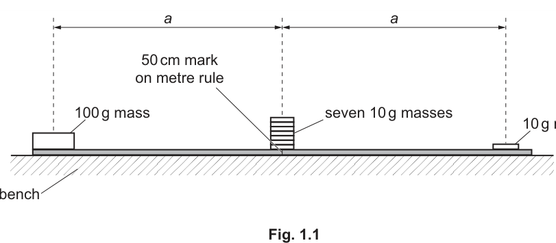
● Place the $100\text{ g}$ mass at one end of the rule.
● The distance between the centre of the $100\text{ g}$ mass and the $50\text{ cm}$ mark on the rule is $a$ .

Measure and record $a$ .

$a$ = ______

● Place a $10\text{ g}$ mass so that its centre is distance $a$ from the $50\text{ cm}$ mark on the rule.
● Secure this mass in place using the adhesive putty. This mass must remain in place throughout the experiment.
● Place seven $10\text{ g}$ masses so that their centres are above the $50\text{ cm}$ mark on the rule.

1M Similar

DifficultyEasy

Worked solution

Answer

Measure $a$ with the metre rule and record to the nearest $1\ \text{mm}$ (or consistent ruler precision).

Example:

a = 50.0\ \text{cm}

Final answer

a = 50.0 cm (example)

Detailed explanation

Background Concept

This part assesses basic experimental measurement skills: measuring a distance along a scale and recording it with sensible precision. A metre rule typically has millimetre divisions, so distances can usually be read to the nearest $1\ \text{mm}$ (i.e. $0.1\ \text{cm}$ ) if the reference point is clear.

Understanding the Question

You are told the $100\ \text{g}$ mass is at one end of the rule, and $a$ is defined as the distance from the centre of that mass to the $50\ \text{cm}$ mark. You must measure and record this distance $a$ .

Approach

Identify the two points: the $50\ \text{cm}$ mark and the centre of the $100\ \text{g}$ mass.
Read the position of the mass centre on the rule scale.
Subtract to obtain $a$ (or measure directly if convenient).
Record $a$ to the correct precision (typically $0.1\ \text{cm}$ ).

Step-by-Step Reasoning

Place the $100\ \text{g}$ mass at the end as instructed and ensure it is positioned consistently.
Locate the centre of the mass (often marked or estimated as the midpoint of its width).
Read the scale value at the centre of the mass, keeping your eye directly above the scale to avoid parallax.
Compute the distance to the $50\ \text{cm}$ mark:

a = |50.0\ \text{cm} - x_{\text{centre}}|

Record the result with appropriate precision, e.g. $a = 50.0\ \text{cm}$ (example).

Key Takeaways

Use clearly defined reference points.
Read scales without parallax.
Record measurements to sensible precision matching the instrument.

Common Mistakes

Measuring from the edge of the mass rather than its centre.
Recording too many decimal places (false precision) or too few (loss of information).
Parallax error from viewing the scale at an angle.

Things to Be Careful About

Ensure the $100\ \text{g}$ mass really is at the end as shown.
If the centre is not marked, estimate it consistently (midpoint of the mass length on the rule).
Use consistent units (usually $\text{cm}$ for metre-rule distances in this practical).

Techniques used

measure a length between two reference points on a scalerecord a measurement to an appropriate precisionavoid parallax by viewing the scale normal to the rule

(b)

● Transfer $n$ of the $10\text{ g}$ masses, where $n = 4$ , from the centre of the rule onto the $10\text{ g}$ mass near the end of the rule.
● Carefully place the rule and masses on the pivot as shown in Fig. 1.2.

Fig. 1.2

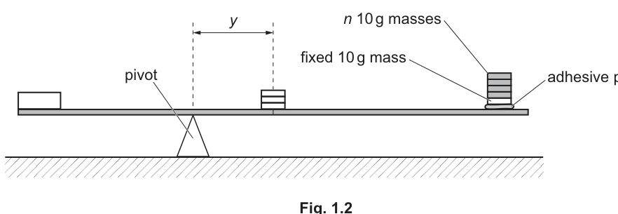
● Adjust the position of the rule on the pivot until the rule is balanced.
● The distance between the pivot and the $50\text{ cm}$ mark on the rule is $y$ .

Record $n$ and $y$ .

$n$ = ______
$y$ = ______

● Remove the rule from the pivot and place it on the bench.
● Return the $n$ $10\text{ g}$ masses to the $50\text{ cm}$ mark.

1M Similar

DifficultyMedium-Easy

Worked solution

Answer

n = 4

Record $y$ (pivot to $50\ \text{cm}$ mark) to nearest $1\ \text{mm}$ (or consistent precision).

Example:

y = 4.20\ \text{cm}

Final answer

n = 4, y = 4.20 cm (example)

Detailed explanation

Background Concept

A balanced rule on a pivot has zero net turning effect (net moment) about the pivot. In practice, you find balance by sliding the rule on the pivot until it stays horizontal (or does not rotate). The measured quantity $y$ is a distance along the rule from a reference mark.

Understanding the Question

You must:

Move $n=4$ of the $10\ \text{g}$ masses from the $50\ \text{cm}$ mark to the fixed $10\ \text{g}$ mass near the end.
Place the rule on the pivot.
Adjust until balanced.
Measure $y$ , defined as the distance between the pivot and the $50\ \text{cm}$ mark.
Record both $n$ and $y$ .

Approach

Set $n=4$ exactly as instructed.
Balance the rule by sliding it carefully on the pivot.
Once balanced, measure $y$ as the separation (along the scale) between the pivot position and the $50\ \text{cm}$ mark.
Record $y$ with appropriate precision.

Step-by-Step Reasoning

Count and transfer exactly four $10\ \text{g}$ masses onto the fixed $10\ \text{g}$ mass.
Place the rule on the pivot. Ensure the pivot contact is sharp (knife-edge) and the rule can rotate freely.
Slide the rule slightly left/right until it remains at rest (not rotating).
Read the position of the pivot on the rule scale (e.g. $x_{\text{pivot}}$ ).
Compute and record

y = |50.0\ \text{cm} - x_{\text{pivot}}|

Example recorded values: $n=4$ , $y=4.20\ \text{cm}$ .

Key Takeaways

Balance first, then measure.
$y$ is measured from the pivot to the $50\ \text{cm}$ mark, not to a mass.
Good technique (free pivot, minimal friction) improves repeatability.

Common Mistakes

Measuring $y$ to the wrong point (e.g. to the end of the rule or to the mass position).
Forgetting that $n$ is fixed at $4$ for this part.
Reading the pivot position with parallax.

Things to Be Careful About

Wait for oscillations to die away before deciding it is balanced.
Ensure masses do not slip when moving the rule.
Record $y$ to a consistent resolution (e.g. $0.1\ \text{cm}$ ).

Techniques used

balance a system on a pivot by adjusting positionmeasure the displacement of a pivot from a reference markrecord repeated measurements consistently

(c)

Change $n$ by moving some of the $10\text{ g}$ masses from the centre of the rule onto the $10\text{ g}$ mass near the end of the rule and determine $y$ .

Repeat until you have six sets of values of $n$ and $y$ .

Record your results in a table.

Include values of $\frac{1}{n}$ and $\frac{y}{n}$ to three significant figures.

9M Similar

DifficultyMedium

Worked solution

Answer

Obtain six pairs of $n$ and $y$ (with a suitable range of $n$ ). Record in one table with headings and units; calculate $1/n$ and $y/n$ to three significant figures.

Example table (illustrative):

$n$	$y / \text{cm}$	$1/n$	$y/n\; / \text{cm}$
2	5.6	0.500	2.80
3	4.9	0.333	1.63
4	4.2	0.250	1.05
5	3.5	0.200	0.700
6	2.8	0.167	0.467
7	2.1	0.143	0.300

Final answer

Student-dependent table of six (n, y) with 1/n and y/n to 3 s.f.

Detailed explanation

Background Concept

In Paper 3, marks are awarded for collecting enough data, using a sensible range, and presenting it correctly. A good results table has:

a single clear table,
correct headings with quantity and unit,
consistent raw-data precision (e.g. all $y$ values to $0.1\ \text{cm}$ ),
derived columns calculated correctly and rounded as instructed (here, three significant figures for $1/n$ and $y/n$ ).

Understanding the Question

You must repeat the balancing procedure for different values of $n$ until you have six sets of $(n, y)$ . Then you must include two calculated columns:

$1/n$ (dimensionless),
$y/n$ (same unit as $y$ , typically $\text{cm}$ ),
rounded to three significant figures.

Approach

Choose six different values of $n$ (a good spread across the allowed range).
For each $n$ : balance the rule and measure $y$ .
Enter $n$ and $y$ into a table immediately.
Compute $1/n$ and $y/n$ and round each to 3 s.f.

Step-by-Step Reasoning

Selecting $n$ values: because you have seven movable $10\ \text{g}$ masses initially at the centre, a natural range is $n=2$ to $n=7$ (or $n=1$ to $n=6$ ), giving six distinct values.
For each chosen $n$ $n$ :
- Move exactly $n$ masses to the fixed mass.
- Balance on the pivot and read $y$ from the pivot to the $50\ \text{cm}$ mark.
Recording in a table:
- Headings should show the quantity and unit, e.g. $y/\text{cm}$ .
- $n$ has no unit.
Calculations:

\frac{1}{n}

and

\frac{y}{n}

Round both to three significant figures (e.g. $1/6 = 0.167$ , not $0.1666\ldots$ ).
Keep $y$ values at consistent precision (e.g. one decimal place if using a mm scale).

Key Takeaways

Collect enough data (six sets) with a sensible range.
Present all data in one clear table.
Apply significant-figure rules carefully to calculated columns.

Common Mistakes

Fewer than six readings.
Missing units in the table heading (especially for $y$ and $y/n$ ).
Mixing precision in one column (e.g. some $y$ values to $0.1\ \text{cm}$ and others to $0.01\ \text{cm}$ ).
Rounding $1/n$ and $y/n$ to three decimal places instead of three significant figures.

Things to Be Careful About

$1/n$ is dimensionless; do not add a unit.
$y/n$ carries the unit of $y$ .
Avoid choosing $n$ values that make balancing impossible (e.g. if at extreme $n$ the rule cannot balance safely).

Techniques used

vary the independent variable over a suitable rangerecord results in a table with correct headings and unitscalculate derived quantities and round to significant figureskeep raw-data precision consistent within columns

(d)

(i)

Plot a graph of $\frac{y}{n}$ on the $y$ -axis against $\frac{1}{n}$ on the $x$ -axis.

3M Similar

DifficultyMedium

Worked solution

Answer

Plot $\dfrac{y}{n}$ on the vertical axis and $\dfrac{1}{n}$ on the horizontal axis.

Axes labelled with quantities and units (e.g. $y/n\; /\ \text{cm}$ , $1/n$ ).
Use a sensible scale (linear, using at least half the grid).
Plot all six points accurately.

Final answer

Graph plotted: y/n vs 1/n

Detailed explanation

Background Concept

A graph is used to reveal and test relationships between variables. Good graph technique in Cambridge practical papers includes:

correct choice of axes as specified,
clear labels (quantity and unit),
sensible scales (not cramped; not awkward such as 3 squares = 1 unit unless unavoidable),
accurate plotting with small, neat crosses.

Understanding the Question

You are told exactly what to plot:

vertical axis: $y/n$ ,
horizontal axis: $1/n$ .
These values come from your table in part (c).

Approach

Compute $1/n$ and $y/n$ (already done in your table).
Draw axes covering most of the grid.
Choose scales that make the points spread out.
Label axes properly.
Plot all six points.

Step-by-Step Reasoning

Put $1/n$ on the x-axis because it is specified as the horizontal variable.
Put $y/n$ on the y-axis.
Axis labels should be like:
- x-axis: $1/n$ (no unit),
- y-axis: $y/n\; /\ \text{cm}$ (or $\text{m}$ if you used metres consistently).
Select scales:
- Find the smallest and largest values of $1/n$ and $y/n$ in your data.
- Pick convenient increments so that the plotted points occupy at least half the grid in both directions.
Plotting:
- Use a sharp pencil.
- Plot each point as a small cross.

Key Takeaways

Always follow the instruction on what to plot.
Labels must include units where appropriate.
Good scale choice is essential for accurate gradient/intercept later.

Common Mistakes

Swapping axes (plotting $1/n$ on y-axis).
Missing units on $y/n$ .
Using a scale that compresses all points into a small corner.
Plotting blobs/dots too large to judge line placement.

Things to Be Careful About

Because $1/n$ values can be recurring decimals (e.g. $0.333$ ), use the rounded values from your table consistently.
Keep units consistent with your measurements of $y$ (cm vs m).

Techniques used

label graph axes with quantity and unitchoose a sensible linear scale using at least half the gridplot points accurately from a results table

(ii)

Draw the straight line of best fit.

1M Similar

(iii)

Determine the gradient and $y$ -intercept of this line.

gradient = ______
$y$ -intercept = ______

2M Similar

DifficultyMedium

Worked solution

Working

Using two well-separated points on the best-fit line,

\text{gradient} = \frac{\Delta (y/n)}{\Delta (1/n)}

Read the $y$ -intercept at $1/n = 0$ from the line.

Example values:

\text{gradient} = 7.0\ \text{cm}

y\text{-intercept} = -0.70\ \text{cm}

Answer

gradient $= 7.0\ \text{cm}$

$y$ -intercept $= -0.70\ \text{cm}$

Final answer

gradient = 7.0 cm, y-intercept = −0.70 cm (example)

Detailed explanation

Background Concept

For a straight-line graph, the gradient and intercept are obtained from the best-fit line, not from individual data points. Gradient is defined by

\text{gradient} = \frac{\Delta y}{\Delta x}

and the y-intercept is the value of $y$ where $x=0$ .

Understanding the Question

You have plotted $y/n$ (vertical) against $1/n$ (horizontal) and drawn a straight best-fit line. You must now determine:

the gradient of this line,
the y-intercept (where the line crosses the vertical axis).

Approach

Choose two points on the line that are far apart (to reduce percentage reading error).
Read their coordinates accurately from the axes.
Compute gradient as $\Delta(y/n) / \Delta(1/n)$ .
Extend the line if needed and read the y-intercept at $1/n = 0$ .

Step-by-Step Reasoning

Pick two points on the line, preferably where it crosses convenient grid intersections.
Suppose the chosen points are $(x_1, y_1)$ $(x_{1}, y_{1})$ and $(x_2, y_2)$ $(x_{2}, y_{2})$ where:
- $x$ represents $1/n$ ,
- $y$ represents $y/n$ .
Then

\text{gradient} = \frac{y_2 - y_1}{x_2 - x_1}

Units:
- $x = 1/n$ is dimensionless,
- $y = y/n$ has the same unit as $y$ (e.g. $\text{cm}$ ),
  so the gradient has units of $\text{cm}$ .
The y-intercept is read at $x=0$ by extending the line to the vertical axis.

Key Takeaways

Use a large triangle and points on the best-fit line.
Gradient is always “change in y over change in x”.
Intercept is where the line crosses the y-axis.

Common Mistakes

Using two experimental points that are not on the best-fit line.
Using $\Delta x/\Delta y$ by accident (inverting the gradient).
Reading intercept from the wrong axis or at the wrong x-value.

Things to Be Careful About

Don’t use small triangles: they magnify reading uncertainties.
Include the sign of the intercept (it can be negative).
Quote values to a sensible number of significant figures based on graph-reading precision (often 2–3 s.f.).

Techniques used

find the gradient using a large triangle on the best-fit linecalculate gradient as $\Delta y / \Delta x$read the y-intercept by extrapolating the best-fit line

(e)

It is suggested that the quantities $y$ and $n$ are related by the equation

\frac{y}{n} = \frac{P}{n} - Q

where $P$ and $Q$ are constants.

Using your answers in (d)(iii), determine the values of $P$ and $Q$ .
Give appropriate units.

$P$ = ______
$Q$ = ______

2M Similar

DifficultyMedium-Easy

Worked solution

Working

Given

\frac{y}{n} = \frac{P}{n} - Q

Let $Y = y/n$ and $X = 1/n$ :

Y = PX - Q

So gradient $= P$ and y-intercept $= -Q$ .

Using (d)(iii) example values:

P = 7.0\ \text{cm}

Q = 0.70\ \text{cm}

Answer

$P = 7.0\ \text{cm}$

$Q = 0.70\ \text{cm}$

Final answer

P = 7.0 cm, Q = 0.70 cm (example)

Detailed explanation

Background Concept

To use a graph to find constants, you rewrite the given relationship into the straight-line form

Y = mX + c

Then:

gradient $m$ gives one constant,
intercept $c$ gives another constant.

Understanding the Question

You are given

\frac{y}{n} = \frac{P}{n} - Q

and you have already found the gradient and y-intercept from the graph of $y/n$ (vertical) against $1/n$ (horizontal). You must use those to determine $P$ and $Q$ , including units.

Approach

Identify which plotted quantities correspond to $Y$ and $X$ .
Rewrite the equation in the form $Y = mX + c$ .
Match $m$ and $c$ to $P$ and $Q$ .
Deduce units of $P$ and $Q$ from the units on the axes.

Step-by-Step Reasoning

Let

Y = \frac{y}{n}, \quad X = \frac{1}{n}

Then

\frac{y}{n} = \frac{P}{n} - Q \;\Rightarrow\; Y = PX - Q

Comparing with $Y = mX + c$ :

gradient $m = P$ ,
intercept $c = -Q$ so $Q = -c$ .

Units:

$X=1/n$ has no units.
$Y=y/n$ has the same units as $y$ (e.g. $\text{cm}$ ).
So:
$P$ (gradient) has units of $Y$ (e.g. $\text{cm}$ ),
$Q$ also has units of $Y$ .

Key Takeaways

Always rewrite into $Y = mX + c$ .
For $Y = PX - Q$ , the intercept is negative: y-intercept $= -Q$ .
Gradient units come from “(units of y-axis)/(units of x-axis)”.

Common Mistakes

Taking $Q$ equal to the intercept instead of the negative of it.
Giving $P$ the wrong units (e.g. $\text{cm}^{-1}$ ) even though $1/n$ is dimensionless.

Things to Be Careful About

Keep the sign of the intercept.
Use the same length unit throughout ( $\text{cm}$ or $\text{m}$ ) so that $P$ and $Q$ are consistent.

Techniques used

compare a straight-line equation to $y = mx + c$identify gradient and intercept with given constantsassign correct units from plotted variables

(f)

Theory suggests that

P = \frac{9Ma}{18M + R}

where $M = 10\text{ g}$ and $R$ is the mass of the rule.

Determine the value of $R$ .

$R$ = ______ $\text{g}$

1M Similar

DifficultyMedium

Worked solution

Working

Given

P = \frac{9Ma}{18M + R}

Rearrange:

P(18M+R)=9Ma

18MP + PR = 9Ma

R = \frac{9Ma}{P} - 18M

Using $M=10\ \text{g}$ and example values $a=50.0\ \text{cm}$ , $P=7.0\ \text{cm}$ :

R = \frac{9\times 10\times 50.0}{7.0} - 18\times 10

R = 4.63\times 10^{2}\ \text{g}

Answer

R = 463\ \text{g}

Final answer

R = 463 g (example)

Detailed explanation

Background Concept

This is using a theoretical model that links the experimentally determined constant $P$ to the mass of the rule $R$ . The key skill is rearranging the formula correctly and substituting values with consistent units.

Understanding the Question

You are given

P = \frac{9Ma}{18M + R}

where:

$M = 10\ \text{g}$ ,
$a$ is your measured distance from part (a),
$P$ comes from part (e),
$R$ is the mass of the rule (unknown).
You must calculate $R$ and give it in grams.

Approach

Rearrange the equation to make $R$ the subject.
Substitute $M$ , your measured $a$ , and your calculated $P$ .
Ensure $a$ and $P$ use the same length unit so they cancel properly.

Step-by-Step Reasoning

Start with

P = \frac{9Ma}{18M + R}

Multiply both sides by $(18M+R)$ :

P(18M+R)=9Ma

Expand:

18MP + PR = 9Ma

Solve for $R$ :

PR = 9Ma - 18MP

R = \frac{9Ma}{P} - 18M

Substitute values (example):

$M=10\ \text{g}$ ,
$a=50.0\ \text{cm}$ ,
$P=7.0\ \text{cm}$ .

Because $a$ and $P$ are both in $\text{cm}$ , they cancel in the fraction $9Ma/P$ , leaving grams, as required.

Key Takeaways

Correct rearrangement is essential: isolate $R$ cleanly before substituting.
Keep $a$ and $P$ in the same length units.
Check that the final unit is $\text{g}$ .

Common Mistakes

Forgetting the bracket when multiplying: treating $P(18M+R)$ as $18MP+R$ .
Using $R = \frac{9Ma}{P} + 18M$ (sign error).
Mixing units (e.g. $a$ in $\text{cm}$ but $P$ in $\text{m}$ ), giving a factor of $100$ error.

Things to Be Careful About

If your y-intercept was negative, you must have used $Q = -\text{intercept}$ in part (e) so that $P$ is correct.
Give $R$ to a sensible precision (often 2–3 s.f.), consistent with the uncertainty in $P$ and $a$ from the experiment.

Techniques used

rearrange an equation to make a target variable the subjectsubstitute measured and derived constants consistentlycheck unit consistency when solving for a mass

Q220MMediumManipulation, Measurement and ObservationAnalysis, Conclusions and EvaluationPresentation of Data and Observations

In this experiment, you will investigate the properties of a rubber band.

(a)

(i)

● Set up the apparatus as shown in Fig. 2.1.

Fig. 2.1

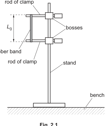
● The rubber band should be straight but not stretched.

The distance between the ends of the rubber band is $L_0$ , as shown in Fig. 2.1.

Measure and record $L_0$ .

$L_0$ = ______

1M Similar

DifficultyEasy

Worked solution

Answer

Measured $L_0$ using a ruler (rubber band straight but not stretched).

Example (to nearest $1\ \text{mm}$ ):

$L_0 = 12.3\ \text{cm}$

Final answer

L0 = 12.3 cm (example)

Detailed explanation

Background Concept

A length measurement should be taken with a suitable instrument (e.g. a ruler or metre rule) and recorded with a precision consistent with the instrument resolution. For a ruler with $1\ \text{mm}$ smallest divisions, a typical reading is recorded to the nearest $1\ \text{mm}$ (or $0.1\ \text{cm}$ ).

Understanding the Question

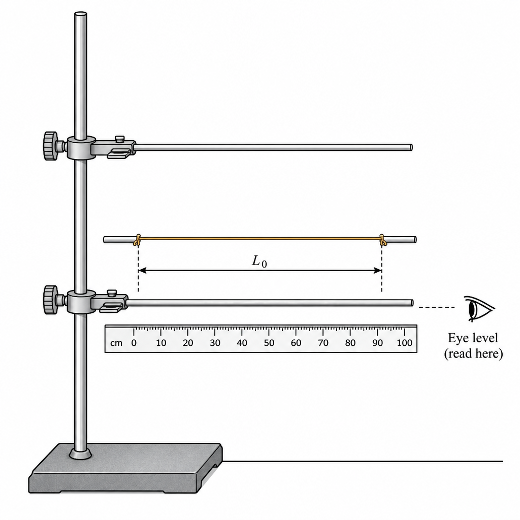
You are asked to measure $L_0$ , the distance between the two ends of the rubber band when it is straight but not stretched (its natural length in the set-up). This is the separation between the attachment points at the clamps/rods.

diagram-2a-i

Approach

Ensure the band is straight and only just taut (no stretch).
Place a ruler parallel to the band.
Read the positions of the two ends (or clamp attachment points) and subtract, or read the separation directly.
Record $L_0$ to the appropriate resolution.

Step-by-Step Reasoning

Check the rubber band is not sagging and not stretched (just straight).
Align the zero (or a convenient mark) of the ruler with one end.
View the scale at eye level to avoid parallax.
Read the length to the nearest division.
Example: if the separation is $12.3\ \text{cm}$ , record $L_0 = 12.3\ \text{cm}$ .

Key Takeaways

Lengths must be recorded with sensible precision matching the instrument.
Good alignment and eye-level reading reduce systematic error.

Common Mistakes

Measuring along a diagonal (ruler not parallel to the band).
Reading the ruler from an angle (parallax).
Recording too many decimal places (false precision).

Things to Be Careful About

Decide what counts as the “end” of the rubber band (consistent reference point at the clamp attachment).
If you measure from two scale readings, remember the uncertainty can be larger than a single reading.
Keep the band straight but not stretched, as instructed.

Techniques used

align a ruler/scale with the measured lengthread a length at eye level to avoid parallaxrecord a measurement to an appropriate resolution

(ii)

Estimate the percentage uncertainty in your value of $L_0$ . Show your working.

percentage uncertainty = ______ $\%$

1M Similar

DifficultyMedium-Easy

Worked solution

Working

Example: $L_0 = 12.3\ \text{cm}$ measured with a ruler to nearest $0.1\ \text{cm}$ , so take $\Delta L_0 = \pm 0.1\ \text{cm}$ .

\%\ \text{uncertainty} = \frac{0.1}{12.3} \times 100 = 0.813\% \approx 0.81\%

Answer

percentage uncertainty $\approx 0.81\%$

Final answer

0.81% (example)

Detailed explanation

Background Concept

Uncertainty in a measured quantity is an estimate of the range within which the true value is likely to lie. For an instrument with finite scale divisions, a common estimate of absolute uncertainty is about half a smallest division for a single reading. If a length is found from two readings (two ends), the absolute uncertainty is often larger because both readings contribute.

Percentage uncertainty is

\%\ \text{uncertainty} = \frac{\text{absolute uncertainty}}{\text{measured value}} \times 100.

Understanding the Question

You must estimate the percentage uncertainty in your measured $L_0$ and show the working. The mark is for a sensible absolute uncertainty and correct conversion to a percentage.

Approach

Decide the absolute uncertainty in $L_0$ based on how you measured it (instrument resolution and number of readings).
Use the percentage uncertainty formula.

Step-by-Step Reasoning

Suppose you used a ruler with $1\ \text{mm}$ divisions and recorded $L_0$ to the nearest $1\ \text{mm}$ (i.e. $0.1\ \text{cm}$ ). A simple acceptable estimate is $\pm 0.1\ \text{cm}$ .
With example $L_0 = 12.3\ \text{cm}$ :

\%\ \text{uncertainty} = \frac{0.1}{12.3} \times 100 = 0.813\%.

Round appropriately: $0.81\%$ .

(If you instead measured by taking two end readings on the ruler and subtracting, you could argue for a larger absolute uncertainty because two readings contribute. The key is to be consistent and show the calculation.)

Key Takeaways

Always state the absolute uncertainty you are using.
Convert to percentage using division then multiply by $100$ .

Common Mistakes

Forgetting to multiply by $100$ .
Mixing units (e.g. using $0.1\ \text{cm}$ with $L_0$ in mm).
Quoting an uncertainty with unrealistic precision.

Things to Be Careful About

If $L_0$ is obtained from two ruler readings, justify whether you used one-reading or two-reading uncertainty.
Keep the uncertainty consistent with how $L_0$ was recorded (nearest mm implies uncertainty of order mm).

Techniques used

estimate absolute uncertainty from instrument resolutioncalculate percentage uncertaintyshow uncertainty working clearly

(b)

The width of the unstretched rubber band is $w_0$ and its thickness is $t$ , as shown in Fig. 2.2.

Fig. 2.2

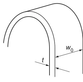
Measure and record $w_0$ and $t$ .

$w_0$ = ______
$t$ = ______

2M Similar

DifficultyMedium-Easy

Worked solution

Answer

Example measurements:

$w_0 = 6.0\ \text{mm}$

$t = 1.20\ \text{mm}$

Final answer

w0 = 6.0 mm, t = 1.20 mm (examples)

Detailed explanation

Background Concept

Width $w_0$ and thickness $t$ are small dimensions, so using instruments with suitable resolution improves precision:

Width can often be measured with vernier calipers (resolution typically $0.01\ \text{cm}$ or $0.1\ \text{mm}$ depending on the instrument) or a ruler if the band is wide enough.
Thickness is better measured with a micrometer screw gauge because $t$ may be around $1\ \text{mm}$ and a ruler is too crude.

When using a micrometer, a common limitation is compressing the rubber; you should gently close the jaws/ratchet to reduce compression error.

Understanding the Question

You need the width of the unstretched rubber band $w_0$ and its thickness $t$ (as shown in the figure). These values are later used in calculations (e.g. force), so they should be recorded clearly with units.

diagram-2b

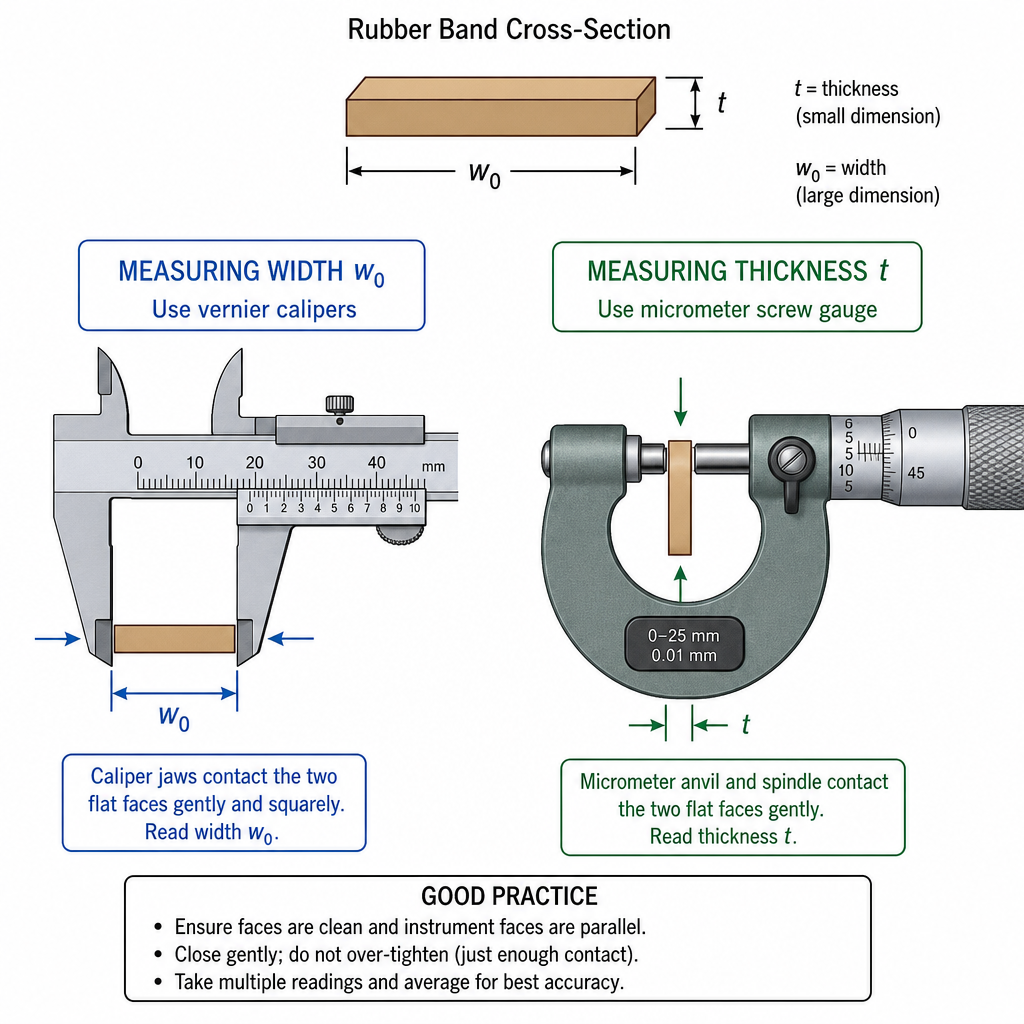
Approach

Measure $w_0$ across the flat face of the band when unstretched.
Measure $t$ across the thickness using a micrometer, using gentle contact.
Record values with appropriate precision and units.

Step-by-Step Reasoning

For $w_0$ : place the jaws of vernier calipers across the band width, ensuring the jaws are perpendicular to the edges. Read and record.
For $t$ : place the band between micrometer anvils and tighten using the ratchet until it just clicks (consistent force). Read and record.
Example outcomes:
- $w_0 = 6.0\ \text{mm}$
- $t = 1.20\ \text{mm}$

Key Takeaways

Choose instruments appropriate to the size of the quantity.
Rubber is compressible: measurement force matters.

Common Mistakes

Measuring thickness with a ruler (too low resolution).
Squeezing the rubber with the micrometer, giving too small $t$ .
Not stating units.

Things to Be Careful About

Measure at the same region each time (rubber band may not be uniform).
If the micrometer has a zero error, correct the readings.
Record consistent decimal places based on instrument resolution.

Techniques used

use calipers or a ruler to measure widthuse a micrometer screw gauge to measure thicknessrecord measurements with appropriate units and precision

(c)

(i)

● Increase the distance between the clamps until the distance between the ends of the rubber band is approximately $1.5L_0$ .
● The distance between the ends of the rubber band is $L$ .

The width of the rubber band is $w$ .

Measure and record $L$ and $w$ .

$L$ = ______
$w$ = ______

1M Similar

DifficultyMedium-Easy

Worked solution

Answer

Example measurements at $L \approx 1.5L_0$ :

$L = 18.5\ \text{cm}$

$w = 5.2\ \text{mm}$

Final answer

L = 18.5 cm, w = 5.2 mm (examples)

Detailed explanation

Background Concept

When a rubber band is stretched, its length increases and its width typically decreases (approximately conserving volume for small strains, though rubber is not perfectly ideal). The experiment requires collecting paired values of $L$ and $w$ for different extensions.

Understanding the Question

You must increase the clamp separation so the end-to-end distance of the rubber band is about $1.5L_0$ , then measure and record:

$L$ : the stretched length (end-to-end)
$w$ : the stretched width

Approach

Use your measured $L_0$ to estimate $1.5L_0$ .
Adjust the clamp separation until the band length is close to that value.
Measure $L$ and then measure $w$ at a consistent location on the band.

Step-by-Step Reasoning

Compute a target length: if $L_0 = 12.3\ \text{cm}$ , then $1.5L_0 \approx 18.45\ \text{cm}$ .
Move one clamp gradually until $L$ is close to this target while the band stays straight.
Measure $L$ with a ruler aligned along the band.
Measure $w$ (preferably with calipers) at the same point along the band each time.
Example: $L = 18.5\ \text{cm}$ , $w = 5.2\ \text{mm}$ .

Key Takeaways

Choose a clear, repeatable point to measure width.
The key practical skill is taking consistent paired readings.

Common Mistakes

Not actually reaching approximately $1.5L_0$ .
Measuring width at different positions along the band.
Allowing the band to twist, changing the apparent width.

Things to Be Careful About

Avoid parallax for $L$ .
Ensure the band is flat (not edge-on) when measuring $w$ .
Record units for each quantity.

Techniques used

adjust apparatus to a target multiple of an initial lengthmeasure the new length and width consistentlyrecord readings with suitable precision

(ii)

Calculate $\Delta L$ and $\Delta w$ , where $\Delta L = L - L_0$ and $\Delta w = w_0 - w$ .

$\Delta L$ = ______
$\Delta w$ = ______

1M Similar

DifficultyMedium-Easy

Worked solution

Working

Using example values: $L = 18.5\ \text{cm}$ , $L_0 = 12.3\ \text{cm}$ , $w_0 = 6.0\ \text{mm}$ , $w = 5.2\ \text{mm}$ .

\Delta L = L - L_0 = 18.5 - 12.3 = 6.2\ \text{cm}

\Delta w = w_0 - w = 6.0 - 5.2 = 0.8\ \text{mm}

Answer

$\Delta L = 6.2\ \text{cm}$

$\Delta w = 0.8\ \text{mm}$

Final answer

ΔL = 6.2 cm, Δw = 0.8 mm (examples)

Detailed explanation

Background Concept

When a question defines derived quantities as differences, you must subtract in the correct order:

\Delta L = L - L_0, \qquad \Delta w = w_0 - w.

For widths, stretching usually makes $w$ smaller than $w_0$ , so $\Delta w$ should be positive if the definition is $w_0 - w$ .

Understanding the Question

You measured $L$ and $w$ at about $1.5L_0$ . Now you must calculate:

$\Delta L$ : how much longer the band is than its initial length
$\Delta w$ : how much the width has decreased

Approach

Subtract the initial value from the new value for length, and subtract the new value from the initial value for width (as specified). Keep units consistent within each subtraction.

Step-by-Step Reasoning

Using the example readings:

Length change:

\Delta L = 18.5\ \text{cm} - 12.3\ \text{cm} = 6.2\ \text{cm}.

Width change:

\Delta w = 6.0\ \text{mm} - 5.2\ \text{mm} = 0.8\ \text{mm}.

These are positive, which matches the expected physical behaviour and the given definitions.

Key Takeaways

Use the definitions exactly as stated.
Subtract values with the same units.

Common Mistakes

Reversing $\Delta w$ as $w - w_0$ (wrong sign).
Mixing cm and mm within one subtraction.
Carrying too many decimal places not justified by measurements.

Things to Be Careful About

Check that $\Delta w$ is not negative; if it is, you may have swapped $w$ and $w_0$ or measured width inconsistently.
Keep derived values to a precision consistent with the raw measurements (see part (c)(iii)).

Techniques used

compute differences using measured valuesmaintain consistent units during subtractionrecord derived quantities clearly

(iii)

Justify the number of significant figures that you have given for your value of $\Delta L$ .

1M Similar

DifficultyMedium-Easy

Worked solution

Answer

$\Delta L$ is found by subtraction ( $\Delta L = L - L_0$ ), so it should be given to the same number of decimal places as the least precise of $L$ and $L_0$ .

Since $L$ and $L_0$ were measured to the nearest $0.1\ \text{cm}$ , $\Delta L$ is quoted to the nearest $0.1\ \text{cm}$ .

Final answer

ΔL quoted to same decimal places as L and L0

Detailed explanation

Background Concept

Significant figures rules depend on the operation:

For multiplication/division, you usually match significant figures.
For addition/subtraction, you match decimal places, because the uncertainty comes from the place value of the last digit.

So for

\Delta L = L - L_0,

$\Delta L$ cannot be more precise (in decimal places) than the least precise of $L$ and $L_0$ .

Understanding the Question

You must explain why you have written $\Delta L$ to a particular number of significant figures/decimal places. The justification must refer to the precision of the measured values used in the subtraction.

Approach

State the subtraction rule (decimal places) and connect it to how $L$ and $L_0$ were recorded from the ruler.

Step-by-Step Reasoning

Suppose $L$ and $L_0$ were both read on a ruler and recorded to the nearest $0.1\ \text{cm}$ .
That means their last reliable digit is in the tenths of a cm.
When subtracting, the uncertainty in the last digit carries through, so $\Delta L$ should also be recorded to the nearest $0.1\ \text{cm}$ .
Example: $18.5\ \text{cm} - 12.3\ \text{cm} = 6.2\ \text{cm}$ , which is indeed to $0.1\ \text{cm}$ .

Key Takeaways

For differences, match decimal places, not significant figures.
Do not overstate precision for derived quantities.

Common Mistakes

Quoting $\Delta L$ to many decimal places because a calculator displays them.
Using the multiplication/division sig-fig rule for subtraction.

Things to Be Careful About

If $L$ and $L_0$ were measured using different instruments/precisions, use the least precise one.
If $\Delta L$ is small compared to $L$ and $L_0$ , percentage uncertainty in $\Delta L$ can be large; still, the recorded decimal places must follow the subtraction rule.

Techniques used

apply subtraction significant-figure (decimal place) rulelink precision of a derived quantity to the least precise measurementstate a clear justification

(d)

● Increase the distance between the clamps until the distance between the ends of the rubber band is approximately $2L_0$ .
● Measure and record $L$ and $w$ .

$L$ = ______
$w$ = ______

● Repeat (c)(ii).

$\Delta L$ = ______
$\Delta w$ = ______

2M Similar

DifficultyMedium-Easy

Worked solution

Working

Example measurements at $L \approx 2L_0$ :

$L = 24.6\ \text{cm}$

$w = 4.6\ \text{mm}$

Using $L_0 = 12.3\ \text{cm}$ and $w_0 = 6.0\ \text{mm}$ :

\Delta L = 24.6 - 12.3 = 12.3\ \text{cm}

\Delta w = 6.0 - 4.6 = 1.4\ \text{mm}

Answer

$L = 24.6\ \text{cm}$ , $w = 4.6\ \text{mm}$

$\Delta L = 12.3\ \text{cm}$ , $\Delta w = 1.4\ \text{mm}$

Final answer

See working (student-dependent); example ΔL = 12.3 cm, Δw = 1.4 mm

Detailed explanation

Background Concept

Collecting data at more than one extension allows you to test a proposed relationship between the changes in dimensions. Repeating the same measurement method at a different extension improves reliability because it checks whether a constant ratio is plausible.

Understanding the Question

You must stretch the band further so that $L \approx 2L_0$ , measure $L$ and $w$ again, then repeat the calculations of $\Delta L$ and $\Delta w$ using the same definitions:

\Delta L = L - L_0, \qquad \Delta w = w_0 - w.

Approach

Estimate the target $2L_0$ .
Adjust the clamp separation to reach that length.
Measure and record $L$ and $w$ as before.
Compute $\Delta L$ and $\Delta w$ .

Step-by-Step Reasoning

Using the same example initial values ( $L_0 = 12.3\ \text{cm}$ , $w_0 = 6.0\ \text{mm}$ ):

Target length is $2L_0 \approx 24.6\ \text{cm}$ .
After adjusting and measuring, suppose:
- $L = 24.6\ \text{cm}$
- $w = 4.6\ \text{mm}$
Now compute changes:

\Delta L = 24.6 - 12.3 = 12.3\ \text{cm},

\Delta w = 6.0 - 4.6 = 1.4\ \text{mm}.

Key Takeaways

Use the same method each time to reduce systematic differences.
Derived quantities must follow the stated definitions.

Common Mistakes

Forgetting to use the original $L_0$ and $w_0$ when calculating changes.
Measuring $w$ at a different location/with the band twisted.

Things to Be Careful About

Rubber can creep (slowly extend) after stretching; take readings consistently (e.g. after waiting a fixed time).
Record $L$ and $w$ to the correct precision for your instruments.

Techniques used

adjust the extension to approximately twice the initial lengthmeasure length and width consistently at a new extensioncalculate changes using defined differences

(e)

It is suggested that the relationship between $\Delta w$ and $\Delta L$ is

\frac{\Delta L}{\Delta w} = k

where $k$ is a constant.

Using your data, calculate two values of $k$ .

first value of $k$ = ______
second value of $k$ = ______

1M Similar

DifficultyMedium-Easy

Worked solution

Working

Convert to consistent units (example):

For $L \approx 1.5L_0$ :

\Delta L = 6.2\ \text{cm} = 0.062\ \text{m}, \qquad \Delta w = 0.8\ \text{mm} = 8.0 \times 10^{-4}\ \text{m}

k_1 = \frac{\Delta L}{\Delta w} = \frac{0.062}{8.0 \times 10^{-4}} = 77.5

For $L \approx 2L_0$ :

\Delta L = 12.3\ \text{cm} = 0.123\ \text{m}, \qquad \Delta w = 1.4\ \text{mm} = 1.4 \times 10^{-3}\ \text{m}

k_2 = \frac{\Delta L}{\Delta w} = \frac{0.123}{1.4 \times 10^{-3}} = 87.9

Answer

first value of $k = 77.5$

second value of $k = 87.9$

Final answer

k1 = 77.5, k2 = 87.9 (examples)

Detailed explanation

Background Concept

If a relationship suggests

\frac{\Delta L}{\Delta w} = k,

then $k$ should be (approximately) constant for different extensions. To test this, you calculate $k$ for two sets of measurements and see if they are close within experimental uncertainty.

Because the ratio involves two lengths, $k$ is dimensionless only if $\Delta L$ and $\Delta w$ are in the same units.

Understanding the Question

You must use your data to calculate two values of $k$ : one from the $\approx 1.5L_0$ stretch and one from the $\approx 2L_0$ stretch.

Approach

For each data set, compute $\Delta L$ and $\Delta w$ (already done in parts (c)(ii) and (d)).
Ensure both are expressed in the same unit (best: convert both to metres).
Compute $k = \Delta L / \Delta w$ for each set.

Step-by-Step Reasoning

Using the example values:

Data set 1:
- $\Delta L = 6.2\ \text{cm} = 0.062\ \text{m}$
- $\Delta w = 0.8\ \text{mm} = 8.0 \times 10^{-4}\ \text{m}$

k_1 = \frac{0.062}{8.0 \times 10^{-4}} = 77.5.

Data set 2:
- $\Delta L = 12.3\ \text{cm} = 0.123\ \text{m}$
- $\Delta w = 1.4\ \text{mm} = 1.4 \times 10^{-3}\ \text{m}$

k_2 = \frac{0.123}{1.4 \times 10^{-3}} = 87.9.

These are not identical (real data rarely is), but the next part asks whether they are consistent given a stated uncertainty.

Key Takeaways

Form ratios in consistent units.
A “constant” in experimental work means “approximately constant within uncertainty”.

Common Mistakes

Using cm for $\Delta L$ and mm for $\Delta w$ without converting (introduces a factor of $10$ error).
Using $\Delta w / \Delta L$ instead of $\Delta L / \Delta w$ .

Things to Be Careful About

Keep enough significant figures in intermediate steps to avoid rounding error, then round sensibly at the end.
If your $\Delta w$ is very small, $k$ will be very sensitive to measurement uncertainty in $w$ .

Techniques used

compute a constant from a ratio of two measured changesuse consistent units when forming a ratiocalculate two values for comparison

(f)

It is suggested that the percentage uncertainty in the values of $k$ is $25\%$ .

Using this uncertainty, explain whether your results support the relationship in (e).

1M Similar

DifficultyMedium

Worked solution

Working

Using example values $k_1 = 77.5$ and $k_2 = 87.9$ with $25\%$ uncertainty:

k_1 = 77.5 \pm 25\% \Rightarrow 77.5 \pm 19.4 \Rightarrow (58.1 \text{ to } 96.9)

k_2 = 87.9 \pm 25\% \Rightarrow 87.9 \pm 22.0 \Rightarrow (65.9 \text{ to } 110)

The ranges overlap.

Answer

Yes. Within $25\%$ uncertainty, the two values of $k$ are consistent, so the results support $\Delta L / \Delta w = k$ .

Final answer

Yes, consistent within 25% so relationship is supported (example).

Detailed explanation

Background Concept

To judge whether two experimental values agree, you compare them using their uncertainties. If each value has an uncertainty band, agreement is indicated when the bands overlap (or when the difference is not larger than the combined uncertainty).

If the percentage uncertainty in $k$ is $25\%$ , then the absolute uncertainty is

\Delta k = 0.25k.

Understanding the Question

You must use the given $25\%$ uncertainty in $k$ to decide whether your two calculated values of $k$ support the idea that $k$ is constant.

Approach

Find the uncertainty range for each $k$ value: $k \pm 0.25k$ .
Check if the ranges overlap.
Conclude whether the data supports a constant $k$ .

Step-by-Step Reasoning

Using example results:

For $k_1 = 77.5$ :

\Delta k_1 = 0.25 \times 77.5 = 19.4,

so acceptable range is $77.5 \pm 19.4$ i.e. $58.1$ to $96.9$ .

For $k_2 = 87.9$ :

\Delta k_2 = 0.25 \times 87.9 = 22.0,

so acceptable range is $87.9 \pm 22.0$ i.e. $65.9$ to $110$ .

Because the intervals overlap (e.g. both include values around $70$ to $95$ ), the two results are consistent within the stated uncertainty. Therefore it is reasonable to say the relationship is supported by the measurements.

Key Takeaways

Uncertainty turns “different numbers” into “possibly consistent results”.
Overlapping uncertainty ranges is a standard practical criterion.

Common Mistakes

Comparing only the raw numbers and concluding “not supported” because they are not equal.
Using $25$ instead of $25\%$ (factor of $100$ error).

Things to Be Careful About

Use the same basis for comparison (either overlap of ranges or difference compared to combined uncertainty).
If your two $k$ values are very far apart compared with $25\%$ , you should conclude the relationship is not supported (and suggest why).

Techniques used

apply a stated percentage uncertainty to create acceptable rangescompare two results using overlapping uncertainty intervalsstate a conclusion consistent with uncertainty

(g)

The approximate force $F$ acting on the rubber band is given by

F = \frac{2Etkw_0 \Delta w}{L_0}

where the Young modulus $E$ of rubber is $1.0 \times 10^6 \text{ N m}^{-2}$ .

Use your second value of $k$ and your value of $\Delta w$ from (d) to determine a value for $F$ .

$F$ = ______ $\text{N}$

1M Similar

DifficultyMedium

Worked solution

Working

Using example values: $E = 1.0 \times 10^6\ \text{N m}^{-2}$ , $t = 1.20\ \text{mm} = 1.20 \times 10^{-3}\ \text{m}$ , $w_0 = 6.0\ \text{mm} = 6.0 \times 10^{-3}\ \text{m}$ , $L_0 = 12.3\ \text{cm} = 0.123\ \text{m}$ .

Second value of $k$ : $k = 87.9$ .

From (d): $\Delta w = 1.4\ \text{mm} = 1.4 \times 10^{-3}\ \text{m}$ .

F = \frac{2Etkw_0 \Delta w}{L_0} = \frac{2(1.0 \times 10^6)(1.20 \times 10^{-3})(87.9)(6.0 \times 10^{-3})(1.4 \times 10^{-3})}{0.123}

F = 14.4\ \text{N}

Answer

$F = 14.4\ \text{N}$

Final answer

14.4 N (example)

Detailed explanation

Background Concept

This part is mainly about correct substitution and unit handling. The force is given by

F = \frac{2Etkw_0\Delta w}{L_0},

where:

$E$ is Young modulus in $\text{N m}^{-2}$ ,
$t$ , $w_0$ , $\Delta w$ , $L_0$ are lengths (must be in $\text{m}$ for SI consistency),
$k$ is the dimensionless ratio from earlier.

If you keep all lengths in metres, the units work out to newtons.

Understanding the Question

You must use:

your second $k$ value (from part (e)), and
your $\Delta w$ from part (d),
plus $E = 1.0 \times 10^6\ \text{N m}^{-2}$ and your measured $t$ , $w_0$ , $L_0$ ,
then calculate $F$ .

Approach

Convert every length quantity to metres.
Substitute carefully into the formula.
Calculate and present $F$ with unit $\text{N}$ .

Step-by-Step Reasoning

Using the example dataset:

Convert to SI:
- $t = 1.20\ \text{mm} = 1.20 \times 10^{-3}\ \text{m}$
- $w_0 = 6.0\ \text{mm} = 6.0 \times 10^{-3}\ \text{m}$
- $\Delta w = 1.4\ \text{mm} = 1.4 \times 10^{-3}\ \text{m}$
- $L_0 = 12.3\ \text{cm} = 0.123\ \text{m}$
Substitute $E = 1.0 \times 10^6$ and $k = 87.9$ :

F = \frac{2(1.0 \times 10^6)(1.20 \times 10^{-3})(87.9)(6.0 \times 10^{-3})(1.4 \times 10^{-3})}{0.123}.

Evaluate stepwise (any equivalent calculator working is fine): result $F \approx 14.4\ \text{N}$ .

Key Takeaways

Convert mm and cm to m before substituting into an SI formula.
Multi-factor formulas are prone to power-of-ten errors; keep track systematically.

Common Mistakes

Leaving one length in mm or cm, giving $F$ wrong by factors of $10$ or $1000$ .
Using the first value of $k$ instead of the second (the question specifies second).
Forgetting the factor of $2$ .

Things to Be Careful About

Ensure $\Delta w$ is in metres, not mm.
Quote a sensible number of significant figures (often 2–3 s.f., consistent with measurements).
Check the result is plausible: stretching a rubber band by hand typically gives forces of order a few newtons to a few tens of newtons.

Techniques used

substitute measured values into a given formulaconvert measurements to SI unitscalculate a numerical result with correct unit

(h)

(i)

Describe four sources of uncertainty or limitations of the procedure for this experiment.
For any uncertainties in measurement that you describe, you should state the quantity being measured and a reason for the uncertainty.

4M Similar

DifficultyMedium

Worked solution

Answer

Any four valid limitations / uncertainties, e.g.

Uncertainty in measuring $L$ and $L_0$ with a ruler: difficulty judging the exact end/attachment point and parallax when reading the scale.
Uncertainty in measuring $w$ and $w_0$ : rubber band may twist or not lie perfectly flat, so the apparent width changes.
Width is not uniform along the band: measuring $w$ at one position may not represent the mean width.
Rubber shows creep/hysteresis: $L$ (and $w$ ) can change with time after stretching, so readings depend on when they are taken.

Final answer

Four limitations listed (see solution).

Detailed explanation

Background Concept

In practical work, uncertainties come from instrument resolution, reading technique, and the behaviour of the system. Limitations are systematic or procedural issues that reduce the validity/reliability of the conclusion (e.g. too few data points, material properties changing with time).

Good answers:

name the quantity affected (e.g. $L$ , $w$ ), and
give a reason (e.g. parallax, difficult reference point, material creep).

Understanding the Question

You must describe four sources of uncertainty or limitations in this rubber band experiment. For measurement uncertainties, you must explicitly state what is being measured and why it is uncertain.

Approach

List four distinct points. Make sure they are not repeats of the same idea (e.g. two different versions of “human error” is not strong). For each, connect to a specific quantity or procedure.

Step-by-Step Reasoning

Examples of creditworthy limitations:

Measuring $L$ and $L_0$ (end-to-end distance):
- The attachment points are not perfectly sharp, so deciding the exact “end” introduces reading uncertainty.
- Parallax error if the ruler is not read at eye level.
Measuring $w$ and $w_0$ (width):
- The rubber band can twist; if it is not perfectly flat, the measured width is underestimated.
- The edges may be curved/irregular, making caliper placement inconsistent.
Non-uniform band geometry:
- Width and thickness can vary along the band; a single-point measurement may not represent the true average cross-section.
Time-dependent rubber behaviour (creep / relaxation / hysteresis):
- After stretching, rubber can continue to extend slowly and its width can change, so $L$ and $w$ depend on how long you wait before measuring.

Other acceptable limitations could include: clamps slipping (changing $L$ ), difficulty keeping the band exactly horizontal/straight, compression error when measuring $t$ with a micrometer, temperature changes affecting rubber properties, and using only two extensions (limited evidence for a relationship).

Key Takeaways

Always connect uncertainty to a specific measurement and a physical cause.
Rubber is a challenging material because it is non-uniform and time-dependent.

Common Mistakes

Writing vague statements like “human error” without specifying what was measured.
Giving fewer than four distinct limitations.
Stating an improvement instead of a limitation.

Things to Be Careful About

Avoid repeating essentially the same point (e.g. parallax for $L$ and parallax for $w$ ) unless clearly different contexts and well explained.
Make sure each point is a limitation of the procedure or measurement, not a random physics fact.

Techniques used

identify measurement uncertainties with a stated quantitylink each limitation to a physical reasondescribe procedural limitations affecting reliability

(ii)

Describe four improvements that could be made to this experiment. You may suggest the use of other apparatus or different procedures.

4M Similar

DifficultyMedium

Worked solution

Answer

Any four valid improvements, e.g.

Use vernier calipers (or a travelling microscope) to measure $w$ and $w_0$ more precisely and consistently, ensuring the band is flat.
Measure $w$ at several positions along the rubber band and take an average to reduce the effect of non-uniform width.
Control timing: take readings after a fixed waiting time after stretching (or pre-stretch the band several times) to reduce creep/hysteresis effects.
Take more than two extensions (e.g. several values of $L$ ) and test the relationship using a graph (e.g. plot $\Delta L$ against $\Delta w$ ) to improve reliability of the conclusion.

Final answer

Four improvements listed (see solution).

Detailed explanation

Background Concept

Improvements are changes that reduce random uncertainty, reduce systematic error, or increase the reliability of the conclusion (e.g. more data points). The best improvements explicitly target a limitation identified in (h)(i).

Understanding the Question

You must describe four improvements to the experiment. You may change apparatus or procedure. The improvements should be practical and clearly linked to better measurements or a stronger test of the relationship.

Approach

Choose four distinct improvements that address different problems:

instrument precision,
consistency/definition of measurement points,
material behaviour (rubber creep),
data quantity/analysis method.

Step-by-Step Reasoning

Examples:

Improve width measurement precision:
- Use vernier calipers or a travelling microscope to measure $w$ and $w_0$ .
- Add a flat backing card behind the band so it stays flat and does not twist during measurement.
Reduce effect of non-uniform width:
- Measure $w$ at 3–5 different positions along the band and average.
- Mark the band at measurement positions to ensure repeatability.
Handle creep/hysteresis:
- Standardise the procedure: wait a fixed time (e.g. 10 s) after adjusting the clamp before reading $L$ and $w$ .
- Pre-condition the rubber band by stretching it through several cycles before taking data, then always stretch in the same direction.
Increase reliability of testing the relationship:
- Take many readings for different values of $L$ (not just $1.5L_0$ and $2L_0$ ).
- Use a graph to test proportionality/constant ratio (a straight-line trend provides stronger evidence than two points).

Other acceptable improvements include: using fixed pointers on clamps to define the “end” points for $L$ , using set squares to align readings, preventing clamp slippage, and controlling temperature.

Key Takeaways

Improvements should be specific, practical, and clearly reduce uncertainty or strengthen the analysis.
More data points generally improves confidence in the conclusion.

Common Mistakes

Repeating the same improvement in different words.
Suggesting an impractical method without describing how it would be implemented.
Giving a limitation again instead of an improvement.

Things to Be Careful About

If you propose a new instrument, state what quantity it measures and how it reduces uncertainty.
If you propose “take more readings”, specify what readings and how they will be analysed (e.g. graph).

Techniques used

propose apparatus changes that reduce measurement uncertaintypropose procedural changes that improve reliabilitypair improvements to corresponding limitations