Physics 9702/33 — February/March 2024

Cambridge AS Level · Advanced Practical Skills · worked solutions for every part, with the mark scheme

questions

marks

120

minutes

Topics Manipulation, Measurement and Observation · Presentation of Data and Observations · Analysis, Conclusions and Evaluation

Q1MediumManipulation, Measurement and ObservationPresentation of Data and ObservationsAnalysis, Conclusions and Evaluation

In this experiment, you will investigate the properties of a pendulum.

(a)

(i)

• Assemble the apparatus as shown in Fig. 1.1 and Fig. 1.2.
• Push the nail through the central hole in the pendulum and then into the plastic tube.
• Secure the tube and nail in the boss, as shown in Fig. 1.1.

Fig. 1.1

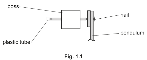
• Ensure that the pendulum swings freely on the nail.

Fig. 1.2

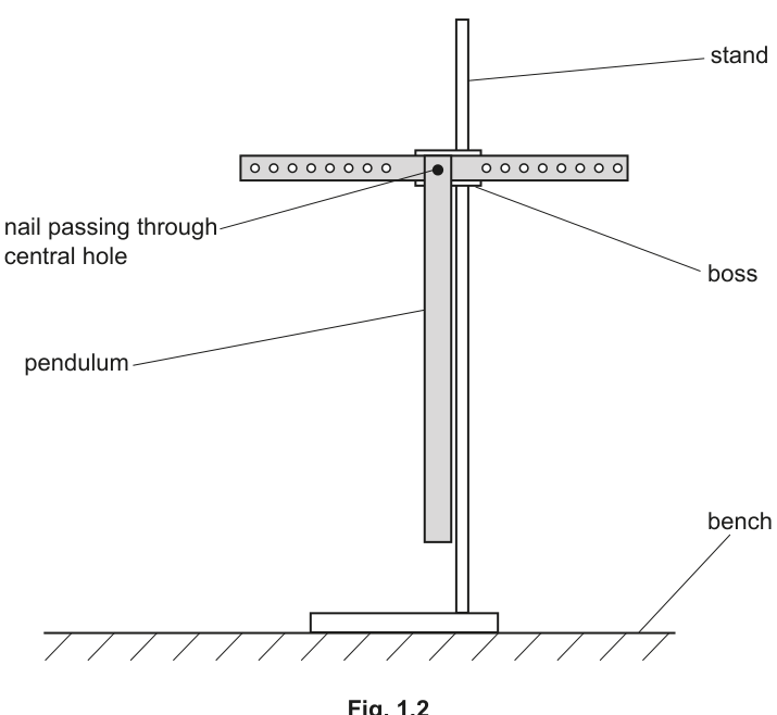
• Attach two 50g slotted masses to the pendulum using the bolts and nuts. Use two holes which are the same distance $x$ from the nail, as shown in Fig. 1.3.

Fig. 1.3

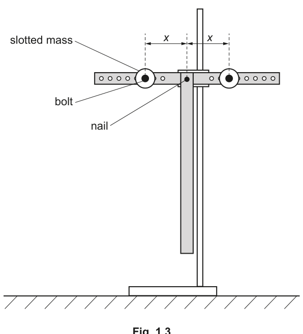
• The distance from the centre of each bolt to the nail is $x$ .
• Measure and record $x$ .

$x$ = ______

1M Similar

DifficultyEasy

Worked solution

Answer

Measure the distance from the nail to the centre of a bolt using a ruler.

Example (to nearest mm):

$x = 12.0\ \text{cm}$

Final answer

x = 12.0 cm (example)

Detailed explanation

Background Concept

In a practical experiment, a length such as $x$ must be defined by two clear reference points and measured with a suitable instrument. A ruler typically reads to $1\ \text{mm}$ , so a measured value should usually be recorded to the nearest $1\ \text{mm}$ (or $0.1\ \text{cm}$ ).

Understanding the Question

You are told that $x$ is the distance from the nail (pivot) to the centre of each bolt/slotted mass. You must measure and record this single distance.

Approach

Decide the two points that define $x$ (pivot nail and bolt centre).
Align a ruler so it measures along the straight line between these points.
Read the scale at the bolt centre and record $x$ with appropriate precision and unit.

Step-by-Step Reasoning

diagram-a-i

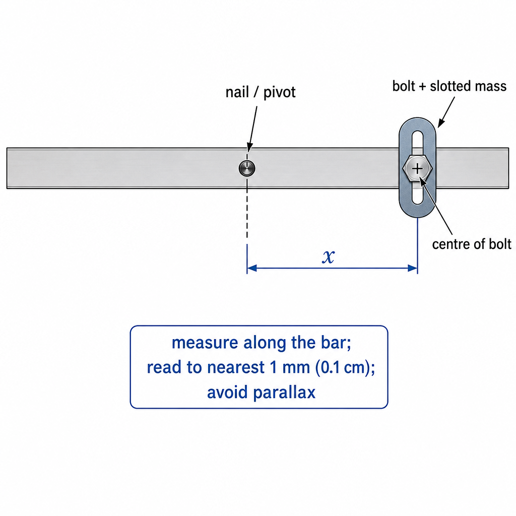
Locate the nail that passes through the pendulum’s central hole (this is the pivot reference).
Locate the centre of the bolt (this is the measurement point on the slotted mass). If the bolt has a circular cross-section, the centre is halfway across the bolt head.
Place the ruler along the pendulum bar so that it lies parallel to the bar and passes through the pivot point and bolt centre.
Avoid parallax: position your eye directly above the ruler markings when reading.
Record $x$ with a unit, typically in cm, to the nearest $0.1\ \text{cm}$ .

A typical recorded value might be $x = 12.0\ \text{cm}$ , but your value depends on which holes were chosen.

Key Takeaways

Always measure between the stated reference points (here: nail to bolt centre).
Record to an appropriate resolution for the instrument (ruler: usually nearest $1\ \text{mm}$ ).

Common Mistakes

Measuring from the edge of the bolt rather than the centre.
Measuring from the boss/tube instead of the nail position.
Recording a value with no unit, or with implausible precision (e.g. $12.034\ \text{cm}$ using a ruler).

Things to Be Careful About

Keep the two masses symmetric, but only one $x$ measurement is required because both should be the same.
Ensure the ruler is aligned along the distance, not at an angle.
Use consistent units throughout the experiment (cm or m) because later you calculate $\sqrt{x^3}$ .

Techniques used

identify the correct reference points for a length measurementuse a ruler to measure a distance with appropriate precisionrecord a measurement with a consistent unit and sensible significant figures

(ii)

Push the bottom of the pendulum a short distance to one side and then release it.
Take measurements to determine the period $T$ of the oscillations.

$T$ = ______

2M Similar

DifficultyMedium-Easy

Worked solution

Working

Time $n$ oscillations ( $n \geq 10$ ) with a stopwatch and repeat.

Example:

\text{time for }10\text{ oscillations} = 14.6\ \text{s}

T = \frac{14.6}{10} = 1.46\ \text{s}

Answer

$T = 1.46\ \text{s}$ (example)

Final answer

T = 1.46 s (example)

Detailed explanation

Background Concept

The period $T$ is the time taken for one complete oscillation. If you time only one oscillation with a hand-operated stopwatch, reaction time gives a large percentage uncertainty. A standard technique is to time a larger number $n$ of oscillations and divide:

T = \frac{t}{n}

Repeating and averaging reduces random error further.

Understanding the Question

You must “take measurements to determine the period $T$ ”. The pendulum is set oscillating with a small displacement and you must obtain a numerical value for the time for one cycle.

Approach

Use a stopwatch.
Count a reasonably large number of complete oscillations (typically $n = 10$ to $20$ ).
Measure total time $t$ for those oscillations.
Compute $T=t/n$ .
Repeat and average $T$ .

Step-by-Step Reasoning

Displace the bottom of the pendulum slightly and release (small amplitude helps keep the motion close to simple harmonic motion and keeps timing consistent).
Choose a clear reference point for counting oscillations, e.g. when the bottom passes a fixed marker moving in the same direction each time.
Start the stopwatch as the pendulum passes the marker, and begin counting oscillations.
Stop the stopwatch after exactly $n$ complete oscillations (same reference point and direction as the start).
Calculate the period:

T = \frac{t}{n}

Example: if $t=14.6\ \text{s}$ for $n=10$ , then $T=1.46\ \text{s}$ .
6. Repeat at least once more and take the mean $T$ for better reliability.

Key Takeaways

Timing many oscillations reduces the fractional effect of reaction time.
Always use a consistent start/stop reference point and direction.
Repeats allow averaging and help spot anomalous results.

Common Mistakes

Timing only one oscillation.
Stopping at the wrong count (e.g. counting half-oscillations instead of full cycles).
Starting and stopping at different points in the motion (introduces systematic differences).

Things to Be Careful About

Keep the amplitude small and similar for each timing.
Avoid pushing the pendulum (release gently) so the motion is in one plane.
Record times to the stopwatch resolution (often $0.01\ \text{s}$ ), but do not overstate precision in the final $T$ beyond what timing uncertainty allows.

Techniques used

time multiple oscillations and divide to obtain the periodreduce random uncertainty by repeating and averaginguse consistent start/stop reference points when timing oscillations

(b)

Vary $x$ by using different holes and measure $T$ .

Repeat until you have six sets of values of $x$ and $T$ .

Record your results in a table. Include values of $\sqrt{x^3}$ in your table.

9M Similar

DifficultyMedium

Worked solution

Answer

Record six sets of $x$ and $T$ (repeat timings and use mean $T$ if taken).
Include a calculated column for $\sqrt{x^3}$ .

Example table (using $x$ in cm):

$x / \text{cm}$	$T / \text{s}$	$\sqrt{x^3} / \text{cm}^{3/2}$
$6.0$	$0.97$	$14.7$
$8.0$	$1.17$	$22.6$
$10.0$	$1.35$	$31.6$
$12.0$	$1.50$	$41.6$
$14.0$	$1.71$	$52.4$
$16.0$	$1.88$	$64.0$

Final answer

Table of 6 readings of x, T, and \sqrt{x^3} (see working/example)

Detailed explanation

Background Concept

A good results table in Paper 3 must:

contain all results in one clear table,
have clear column headings with quantity and unit (e.g. $x/\text{cm}$ ),
show raw values to a consistent precision,
include calculated quantities with sensible significant figures.

Here the independent variable is $x$ and the dependent variable is $T$ . You are also asked to calculate $\sqrt{x^3}$ , which is the same as $x^{3/2}$ .

Understanding the Question

You must change $x$ by using different holes, measure the period $T$ each time, and obtain six pairs of $(x, T)$ . You must then present these results in a table and add a third column containing $\sqrt{x^3}$ for each $x$ value.

Approach

Choose six different hole positions spanning a good range of $x$ values (not clustered).
For each $x$ , measure $x$ carefully and determine $T$ by timing many oscillations.
Compute $\sqrt{x^3}$ for each $x$ using a calculator.
Present all values in a single table with correct headings, units, and consistent decimal places.

Step-by-Step Reasoning

Pick six values of $x$ (e.g. $6.0, 8.0, 10.0, 12.0, 14.0, 16.0\ \text{cm}$ ). A wide spread improves the graph and helps determine gradient accurately.
For each $x$ , time $n$ oscillations (e.g. $n=10$ or $20$ ), repeat, and take a mean period $T$ .
Calculate the derived quantity:

\sqrt{x^3} = (x^3)^{1/2} = x^{3/2}

For example, if $x=12.0\ \text{cm}$ :

\sqrt{x^3} = \sqrt{(12.0)^3} = \sqrt{1728} = 41.6\ \text{cm}^{3/2}

Table conventions:

Put $x$ and $T$ as measured columns.
Put $\sqrt{x^3}$ as a calculated column.
Keep decimal places consistent within a column (e.g. $x$ to $0.1\ \text{cm}$ throughout).

Key Takeaways

Six well-spaced readings give a better straight-line graph than values that are close together.
A derived column must be clearly labelled with its unit.
Consistent precision is a marking point in practical papers.

Common Mistakes

Missing units in the headings.
Splitting results across multiple tables.
Inconsistent decimal places (e.g. $x=6, 8.0, 10.00$ ).
Calculating $\sqrt{x^3}$ incorrectly (e.g. using $\sqrt{x}$ or $x^3$ instead).

Things to Be Careful About

If you decide to use SI units (m) for $x$ , then all $x$ values and $\sqrt{x^3}$ values must be in m and $\text{m}^{3/2}$ respectively.
Do not round intermediate calculator steps too early; round the final derived value appropriately (usually 3 s.f. is acceptable if $x$ is to 3 s.f.).
Ensure the pendulum swings freely and in one plane for every reading so that changes in $T$ are due to changing $x$ , not friction or twisting.

Techniques used

select a suitable range and number of values for the independent variablerecord raw measurements in a single table with headings and unitscalculate a derived quantity from measured data using consistent significant figuresrepeat measurements and use mean values where appropriate

(c)

(i)

Plot a graph of $T$ on the $y$ -axis against $\sqrt{x^3}$ on the $x$ -axis.

3M Similar

DifficultyMedium-Easy

Worked solution

Answer

Plot $T$ on the $y$ -axis and $\sqrt{x^3}$ on the $x$ -axis.

Label axes: $T/\text{s}$ and $\sqrt{x^3}/\text{cm}^{3/2}$ (or consistent units used).
Use a sensible scale (at least half the grid in each direction).
Plot all six points accurately with small crosses.

Final answer

Graph plotted: T vs \sqrt{x^3} with correct axes/units and points

Detailed explanation

Background Concept

Graphs in Paper 3 are assessed on presentation as well as accuracy. Marks are typically awarded for:

correct choice of axes (correct variables),
correct axis labels including units,
sensible scales that use much of the graph paper,
accurate plotting of points.

Understanding the Question

You are told exactly what to plot: $T$ on the vertical axis against $\sqrt{x^3}$ on the horizontal axis. This means $\sqrt{x^3}$ is treated as the independent variable for the graph.

Approach

Decide which units you used in your table (cm or m) and keep them the same on the graph.
Choose scales so that the smallest and largest values of both quantities fit well and spread across most of the grid.
Plot each data pair $(\sqrt{x^3},\,T)$ as a small cross.

Step-by-Step Reasoning

From your table, read off the minimum and maximum of $\sqrt{x^3}$ and $T$ .
On the $x$ -axis write the label $\sqrt{x^3} / \text{cm}^{3/2}$ (or $\text{m}^{3/2}$ if using SI).
On the $y$ -axis write the label $T / \text{s}$ .
Choose a linear scale (not awkward such as 3 squares = 1 unit) and aim to use at least half the available axis length.
Plot each point carefully: align with grid lines, use a sharp pencil, and make a small cross rather than a dot.

Key Takeaways

Always include both quantity and unit in axis labels.
Scale choice matters: a good spread improves gradient accuracy.

Common Mistakes

Plotting $x$ instead of $\sqrt{x^3}$ .
Missing units on one or both axes.
Choosing a scale that compresses the points into a small region.

Things to Be Careful About

Do not force the graph through the origin unless justified by the data/relationship.
Ensure you plot $\sqrt{x^3}$ values that correspond to the same $x$ values used for each $T$ measurement.

Techniques used

choose suitable axis scales that use most of the graph gridlabel axes with quantity and unitplot experimental points accurately using small crosses

(ii)

Draw the straight line of best fit.

1M Similar

(iii)

Determine the gradient and $y$ -intercept of this line.

gradient = ______
y-intercept = ______

2M Similar

DifficultyMedium

Worked solution

Working

Using two well-separated points on the best-fit line, e.g.

(\sqrt{x^3}, T) = (20.0, 1.10)\ \text{and}\ (70.0, 2.35)

\text{gradient} = \frac{\Delta T}{\Delta (\sqrt{x^3})} = \frac{2.35 - 1.10}{70.0 - 20.0} = \frac{1.25}{50.0} = 0.0250

b = \text{y-intercept} = 1.10 - (0.0250)(20.0) = 0.60\ \text{s}

Answer

$\text{gradient} = 0.0250\ \text{s cm}^{-3/2}$

$\text{y-intercept} = 0.60\ \text{s}$

Final answer

gradient = 0.0250 s cm^{-3/2}, y-intercept = 0.60 s (example)

Detailed explanation

Background Concept

For a straight-line graph of the form $y=mx+c$ :

the gradient is $m = \Delta y / \Delta x$ ,
the y-intercept is $c$ (the value of $y$ where $x=0$ ).

Units:

$m$ has units of (units of $y$ )/(units of $x$ ),
$c$ has the same units as $y$ .

Understanding the Question

Your graph has $T$ on the $y$ -axis and $\sqrt{x^3}$ on the $x$ -axis. You must find:

the gradient of the best-fit line,
the y-intercept (where the line crosses the $T$ -axis).

Approach

Use a large triangle on the best-fit line (not between two raw data points unless they lie on the line).
Read two points on the line as accurately as possible.
Compute gradient using $\Delta T / \Delta(\sqrt{x^3})$ .
Determine y-intercept by reading where the line meets the $T$ -axis (or by substituting one point into $T = m(\sqrt{x^3}) + c$ ).

Step-by-Step Reasoning

diagram-c-iii

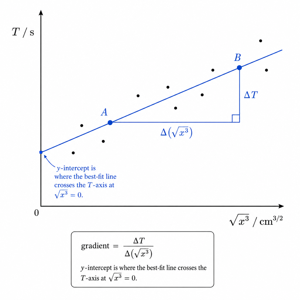
Choose two points far apart on the best-fit line to reduce percentage reading error. For example, pick one point near the left and one near the right.
Read their coordinates: $(x_1, y_1)$ and $(x_2, y_2)$ where $x$ represents $\sqrt{x^3}$ and $y$ represents $T$ .
Calculate:

\text{gradient} = m = \frac{y_2-y_1}{x_2-x_1}

Attach units:

if $T$ is in s and $\sqrt{x^3}$ is in $\text{cm}^{3/2}$ , then

[m] = \frac{\text{s}}{\text{cm}^{3/2}} = \text{s cm}^{-3/2}

Find y-intercept $c$ :

either read it directly at $x=0$ on the graph,
or calculate it using one point on the best-fit line:

c = y_1 - mx_1

It must have units of seconds.

Key Takeaways

Always use a large triangle on the best-fit line for gradient.
Gradient units come from y-units divided by x-units.
The intercept is where the line crosses the y-axis, not where the first data point lies.

Common Mistakes

Using two experimental points that are not on the best-fit line.
Calculating $\Delta x / \Delta y$ instead of $\Delta y / \Delta x$ .
Forgetting units, or giving intercept units that are not seconds.

Things to Be Careful About

Read coordinates from the line, not from nearby points.
Use at least half the graph width/height for your gradient triangle.
If your line does not reach $x=0$ on the graph, extend it carefully with a ruler to read the intercept.

Techniques used

construct a large gradient triangle on a best-fit linecalculate gradient using \Delta y / \Delta x with unitsread the y-intercept from the best-fit line at x = 0

(d)

It is suggested that the quantities $T$ and $x$ are related by the equation

T = a \sqrt{x^3} + b

where $a$ and $b$ are constants.

Using your answers in (c)(iii), determine the values of $a$ and $b$ .
Give appropriate units.

$a$ = ______
$b$ = ______

2M Similar

DifficultyMedium-Easy

Worked solution

Working

Given

T = a\sqrt{x^3} + b

Comparing with $y = mx + c$ for a graph of $T$ (y-axis) against $\sqrt{x^3}$ (x-axis):

a = \text{gradient},\quad b = \text{y-intercept}

Answer

$a = 0.0250\ \text{s cm}^{-3/2}$

$b = 0.60\ \text{s}$

Final answer

a = gradient, b = y-intercept (with appropriate units)

Detailed explanation

Background Concept

If you plot a graph and obtain a straight line, you can compare the experimental straight-line equation with the theoretical model.

For a graph of $y$ against $x$ :

y = mx + c

where $m$ is the gradient and $c$ is the y-intercept.

Understanding the Question

The suggested relationship is:

T = a\sqrt{x^3} + b

You already plotted $T$ against $\sqrt{x^3}$ and found the gradient and y-intercept in part (c)(iii). You now must use those to state $a$ and $b$ , including units.

Approach

Identify what plays the role of $y$ and $x$ .
Match coefficients:
- coefficient of $\sqrt{x^3}$ is the gradient,
- constant term is the y-intercept.
Assign units based on the units used on the graph.

Step-by-Step Reasoning

Your graph is $T$ (vertical) versus $\sqrt{x^3}$ (horizontal).
So the straight-line form is:

T = (\text{gradient})\,(\sqrt{x^3}) + (\text{y-intercept})

Comparing with $T = a\sqrt{x^3} + b$ gives:

a = \text{gradient},\quad b = \text{y-intercept}

Units:

$b$ must have the same units as $T$ , i.e. seconds.
$a$ must be $\text{s}$ divided by the units of $\sqrt{x^3}$ . If $x$ was measured in cm, then $\sqrt{x^3}$ is in $\text{cm}^{3/2}$ , so:

[a] = \text{s cm}^{-3/2}

(If you used metres instead, then $[a]=\text{s m}^{-3/2}$ .)

Key Takeaways

When you plot $T$ against $\sqrt{x^3}$ , the gradient directly gives the constant multiplying $\sqrt{x^3}$ .
The y-intercept gives the additive constant.
Units come from comparing the plotted quantities.

Common Mistakes

Swapping $a$ and $b$ .
Giving $b$ the same units as $a$ (it must be seconds).
Using the wrong unit power for $a$ (it must include $\text{(length)}^{-3/2}$ ).

Things to Be Careful About

Units depend on what you actually used for $x$ (cm or m). Use the same system consistently.
If your graph was not perfectly linear, use the best-fit line values of gradient/intercept, not values from a single pair of raw points.

Techniques used

match a straight-line equation to y = mx + cidentify constants from gradient and interceptdeduce the correct units of constants from the plotted variables

Q2MediumManipulation, Measurement and ObservationAnalysis, Conclusions and EvaluationPresentation of Data and Observations

In this experiment, you will investigate the frictional forces on a wooden strip.

(a)

(i)

• You have been provided with two wooden strips. Select the thicker strip.
Measure and record its length $L$ .

$L$ = ______ $\text{cm}$

• Attach the slotted mass to one of the wider faces of the strip approximately $10\ \text{cm}$ from one end using a small piece of adhesive putty, as shown in Fig. 2.1.

Fig. 2.1

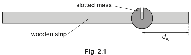
• The distance from the centre of the slotted mass to the nearest end of the strip is $d_A$ , as shown in Fig. 2.1.

Measure and record $d_A$ .

$d_A$ = ______ $\text{cm}$

2M Similar

DifficultyMedium-Easy

Worked solution

Measure $L$ with a metre rule (to nearest $0.1\ \text{cm}$ ).

Example: $L = 60.0\ \text{cm}$ .

Measure $d_A$ from the nearest end of the strip to the centre of the slotted mass (to nearest $0.1\ \text{cm}$ ).

Example: $d_A = 10.0\ \text{cm}$ .

Final answer

Example: L = 60.0 cm, dA = 10.0 cm

Detailed explanation

Background Concept

In practical work, length measurements should be made with (i) a clear definition of the endpoints being used, and (ii) a suitable instrument and precision. A metre rule typically allows readings to $\pm 0.05\ \text{cm}$ (if read to the nearest $0.1\ \text{cm}$ ) provided parallax is avoided.

Here, $L$ is the total strip length, and $d_A$ is a distance to the centre of the slotted mass, so you must decide where “centre” is (usually the midpoint of the slotted mass along the strip).

Understanding the Question

You are told to choose the thicker strip, then:

measure and record its length $L$ in $\text{cm}$ ,
attach the slotted mass about $10\ \text{cm}$ from one end,
measure $d_A$ : distance from the centre of the mass to the nearest end.

Marks are awarded for sensible measurements and correct recording (unit, precision).

Approach

Use a metre rule to measure $L$ with the strip flat on the bench.
After attaching the mass, locate the centre of the mass along the strip.
Measure from the nearer end of the strip to that centre to obtain $d_A$ .
Record both values with consistent precision (e.g. 0.1 cm) and unit.

Step-by-Step Reasoning

Place the strip so that one end aligns with the metre rule zero. Read the other end at eye level to avoid parallax. Record $L$ .
Attach the slotted mass using a small amount of putty so it does not noticeably shift.
Decide the centre position of the mass (e.g. halfway along its length). If the mass has a clear midpoint, use that; otherwise measure its length and halve it.
Measure the distance from the centre point to the nearest end of the strip, again reading the scale at eye level.

A typical set of readings might be $L = 60.0\ \text{cm}$ and $d_A = 10.0\ \text{cm}$ (your values will differ).

Key Takeaways

Define exactly what points you measure between (especially “centre of mass”).
Use consistent precision and include units.
Reduce parallax by reading scales at eye level.

Common Mistakes

Measuring $d_A$ to the edge of the mass rather than its centre.
Recording $L$ and $d_A$ with mismatched precision (e.g. one to nearest cm, the other to 0.1 cm).
Forgetting units.

Things to Be Careful About

Ensure the mass is attached approximately $10\ \text{cm}$ from an end (as instructed), but still measure the actual $d_A$ rather than assuming it is $10\ \text{cm}$ .
Ensure the strip end is aligned with the zero of the rule; if not, subtract the two end readings correctly.

Techniques used

measure length with a metre rule to appropriate precisionidentify the centre of the slotted mass to define the distancerecord readings with consistent units and decimal places

(ii)

You have been provided with a smooth board. Support the board vertically on the bench using the stand, boss and clamp, as shown in Fig. 2.2.

Fig. 2.2

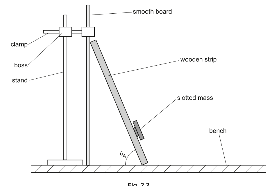
• Lean the strip against the smooth board with the slotted mass nearer the lower end, as shown in Fig. 2.2.
• Move the bottom of the strip away from the smooth board until the strip starts to slip. Gradually push the bottom of the strip back towards the board until it just stays in position by itself.
• The angle between the strip and the bench is $\theta_A$ , as shown in Fig. 2.2.

Measure and record $\theta_A$ .

$\theta_A$ = ______ $^{\circ}$

2M Similar

DifficultyMedium-Easy

Worked solution

Adjust the bottom of the strip until it is just not slipping, then measure the angle $\theta_A$ between strip and bench with a protractor.

Example: $\theta_A = 35^\circ$ .

Final answer

Example: θA = 35°

Detailed explanation

Background Concept

When an object is on the point of slipping, static friction is at (or very near) its maximum value. This “limiting equilibrium” condition is often hard to judge, so the procedure uses a method of overshooting (make it slip) and then returning slowly to the threshold where it just stays.

The angle $\theta_A$ is defined as the angle between the strip and the horizontal bench.

Understanding the Question

You must:

set up the vertical smooth board with the clamp,
lean the strip with the mass nearer the lower end,
find the position where the strip is just self-supporting (not slipping),
measure and record $\theta_A$ .

The key difficulty is judging the “just stays” condition and reading the angle without parallax.

Approach

Set the board vertical and stable.
Place the strip against the board in the required orientation.
Find the critical position by moving the bottom out to make it slip, then moving it back slowly until it just remains at rest.
Measure $\theta_A$ with a protractor (angle between strip and bench).

Step-by-Step Reasoning

Ensure the smooth board is vertical (a slight tilt changes the contact forces).
With the strip leaning, move the bottom away until slipping occurs (this confirms you are beyond the threshold).
Slowly push the bottom back towards the board until it just stops slipping and remains in place.
Place a protractor with its baseline along the bench (horizontal). Read the angle to the strip, ideally aligning the protractor’s centre at the contact point on the bench.

A typical value might be $\theta_A = 35^\circ$ .

Key Takeaways

The “just stays” condition is a limiting equilibrium point.
Angle measurement needs correct reference (bench) and careful reading.

Common Mistakes

Measuring the angle to the vertical board instead of to the bench.
Reading the angle when the strip is still creeping/slipping.
Holding the strip while measuring (this changes the forces).

Things to Be Careful About

Keep the strip and board surfaces clean; contamination changes friction unpredictably.
Avoid bumping the bench during the measurement; vibrations can trigger slipping near the threshold.

Techniques used

adjust the strip to the limiting equilibrium conditionmeasure an angle using a protractor relative to the horizontal benchrepeat the adjustment to identify the just-stable position

(iii)

Estimate the percentage uncertainty in your value of $\theta_A$ .
Show your working.

percentage uncertainty = ______ $\%$

1M Similar

DifficultyMedium-Easy

Worked solution

Assume protractor uncertainty $= \pm 1^\circ$ .

\%\ \text{uncertainty} = \frac{1^\circ}{\theta_A} \times 100

Using $\theta_A = 35^\circ$ :

\%\ \text{uncertainty} = \frac{1}{35} \times 100 = 2.86\% \approx 2.9\%

Final answer

2.9% (example, using ±1°)

Detailed explanation

Background Concept

An uncertainty estimate reflects the likely range in which the true value lies. For direct readings from an analogue scale (like a protractor), a common estimate is about half a smallest division, or sometimes $\pm 1^\circ$ to account for alignment and parallax.

Percentage uncertainty is calculated by

\%\ \text{uncertainty} = \frac{\text{absolute uncertainty}}{\text{measured value}}\times 100

Understanding the Question

You must estimate the percentage uncertainty in your measured $\theta_A$ and show working. The question expects you to:

state an absolute uncertainty in degrees,
divide by your measured angle,
multiply by 100 to get a percentage.

Approach

Choose a sensible absolute uncertainty for your angle measurement (typically $\pm 1^\circ$ for a protractor reading in this setup).
Use the percentage uncertainty formula.
Substitute your measured $\theta_A$ .

Step-by-Step Reasoning

Suppose your protractor scale is marked in $1^\circ$ divisions. In practice, alignment with the strip and locating the exact vertex adds extra uncertainty, so $\pm 1^\circ$ is reasonable.
With $\theta_A = 35^\circ$ :

\%\ \text{uncertainty} = \frac{1}{35} \times 100 = 2.86\% \approx 2.9\%

If your own $\theta_A$ differs, your percentage will change accordingly.

Key Takeaways

Percentage uncertainty depends on both instrument precision and the size of the reading.
Always show absolute uncertainty and the calculation.

Common Mistakes

Using $\theta_A/1$ instead of $1/\theta_A$ .
Giving an uncertainty without stating what absolute uncertainty was assumed.
Forgetting the factor of 100.

Things to Be Careful About

If you justify a different absolute uncertainty (e.g. $\pm 0.5^\circ$ ), keep it consistent with the protractor resolution and your ability to align the strip.
Use the same $\theta_A$ value as you recorded in (a)(ii).

Techniques used

estimate absolute uncertainty from instrument resolutioncalculate percentage uncertainty using ratio times 100show uncertainty working clearly

(iv)

The mass of the thicker strip is $M$ . The value of $M$ is written on the strip.

• Record $M$ .

$M$ = ______ $\text{g}$

• Calculate $F_A$ using

F_A = \frac{\frac{M}{2} + \frac{Sd_A}{L}}{(M + S) \tan \theta_A}

where $S$ is $100\ \text{g}$ .

$F_A$ = ______

1M Similar

DifficultyMedium-Easy

Worked solution

Record mass of thicker strip (value on strip). Example: $M = 150\ \text{g}$ .

F_A = \frac{\frac{M}{2} + \frac{Sd_A}{L}}{(M+S)\tan\theta_A}

Using $S=100\ \text{g}$ , $M=150\ \text{g}$ , $d_A=10.0\ \text{cm}$ , $L=60.0\ \text{cm}$ , $\theta_A=35^\circ$ :

F_A = \frac{75.0 + \frac{100\times 10.0}{60.0}}{(150+100)\tan 35^\circ} = \frac{75.0 + 16.7}{250\times 0.700} = \frac{91.7}{175} = 0.524

Final answer

Example: M = 150 g, FA = 0.524

Detailed explanation

Background Concept

In many practical questions, you are given a formula that turns measured quantities into a derived result. Marks are earned for:

recording the measured quantity ( $M$ ) correctly,
substituting correctly with consistent units,
producing a sensible numerical result to appropriate significant figures.

The expression involves $\tan\theta_A$ , so the angle must be in degrees (as measured) when using a calculator in degree mode.

Understanding the Question

You must:

Read $M$ (mass of the thicker strip) from the writing on the strip and record it in $\text{g}$ .
Calculate $F_A$ using the given equation, with $S=100\ \text{g}$ and your measured $L$ , $d_A$ , and $\theta_A$ .

Approach

Copy the given formula.
Substitute your measured values.
Calculate numerator and denominator separately to reduce errors.
Quote $F_A$ to 3 s.f. (typical for calculated results in Paper 3 unless otherwise indicated).

Step-by-Step Reasoning

Using the example set of measurements:

$M = 150\ \text{g}$ (read directly from the strip)
$S=100\ \text{g}$ (given)
$d_A=10.0\ \text{cm}$ , $L=60.0\ \text{cm}$
$\theta_A = 35^\circ$

Compute the numerator:

\frac{M}{2} + \frac{Sd_A}{L} = 75.0 + \frac{100\times 10.0}{60.0} = 75.0 + 16.7 = 91.7

Compute the denominator:

(M+S)\tan\theta_A = (150+100)\tan 35^\circ = 250\times 0.700 = 175

Then

F_A = \frac{91.7}{175} = 0.524

Your own $F_A$ will depend on your recorded $M$ , $L$ , $d_A$ , and $\theta_A$ .

Key Takeaways

Substitute carefully and keep units consistent with the formula.
Use calculator in degree mode for $\tan$ of a degree angle.

Common Mistakes

Using $\tan$ in radian mode.
Mixing units (e.g. using $L$ in m but $d_A$ in cm).
Forgetting that $S=100\ \text{g}$ must be included.

Things to Be Careful About

Brackets: ensure $(M+S)$ multiplies $\tan\theta_A$ .
Significant figures: do not over-round intermediate values; round at the end.

Techniques used

substitute measured values into a provided equationevaluate a trigonometric function in a calculationrecord a calculated quantity to appropriate significant figures

(v)

• Invert the thicker strip and lean it against the smooth board so that the slotted mass is nearer the upper end as shown in Fig. 2.3.

Fig. 2.3

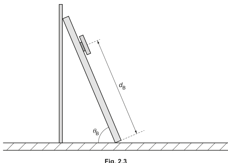
• The distance from the centre of the slotted mass to the lower end of the strip is $d_B$ .

Measure and record $d_B$ .

$d_B$ = ______ $\text{cm}$

• Move the bottom of the strip away from the smooth board until the strip starts to slip. Gradually push the bottom of the strip back towards the board until it just stays in position by itself.
• The angle between the strip and the bench is $\theta_B$ , as shown in Fig. 2.3.

Measure and record $\theta_B$ .

$\theta_B$ = ______ $^{\circ}$

• Calculate $F_B$ , using

F_B = \frac{\frac{M}{2} + \frac{Sd_B}{L}}{(M + S) \tan \theta_B}

$F_B$ = ______

1M Similar

DifficultyMedium

Worked solution

Measure $d_B$ (to nearest $0.1\ \text{cm}$ ). Example: $d_B = 50.0\ \text{cm}$ .

Adjust until the strip just stays and measure $\theta_B$ . Example: $\theta_B = 55^\circ$ .

F_B = \frac{\frac{M}{2} + \frac{Sd_B}{L}}{(M+S)\tan\theta_B}

Using $S=100\ \text{g}$ , $M=150\ \text{g}$ , $d_B=50.0\ \text{cm}$ , $L=60.0\ \text{cm}$ , $\theta_B=55^\circ$ :

F_B = \frac{75.0 + \frac{100\times 50.0}{60.0}}{250\tan 55^\circ} = \frac{75.0 + 83.3}{250\times 1.43} = \frac{158.3}{357} = 0.444

Final answer

Example: dB = 50.0 cm, θB = 55°, FB = 0.444

Detailed explanation

Background Concept

Repeating the experiment with the strip inverted changes the torque balance due to the shifted position of the slotted mass relative to the ends, so the critical angle $\theta$ changes. You then use the provided formula to compute a corresponding derived quantity ( $F_B$ ).

Understanding the Question

You must:

invert the strip so the mass is nearer the upper end,
measure $d_B$ (centre of mass to the lower end),
adjust to the “just stays” position and measure $\theta_B$ ,
calculate $F_B$ using the given expression.

Approach

Reconfigure exactly as instructed (mass nearer the upper end).
Measure $d_B$ to the centre of the mass, with the correct reference end.
Find the limiting position (just not slipping) and measure $\theta_B$ .
Substitute into the equation for $F_B$ .

Step-by-Step Reasoning

When measuring $d_B$ , ensure you measure to the lower end (as stated) and to the centre of the mass.
Finding the “just stays” angle is the same technique as in (a)(ii): make it slip, then move back slowly until it just remains at rest.
Substitute into

F_B = \frac{\frac{M}{2} + \frac{Sd_B}{L}}{(M+S)\tan\theta_B}

Using the example numbers:

\text{numerator} = 75.0 + \frac{100\times 50.0}{60.0} = 75.0 + 83.3 = 158.3

\text{denominator} = 250\tan 55^\circ = 250\times 1.43 = 357

F_B = \frac{158.3}{357} = 0.444

Key Takeaways

After inversion, re-check which end is “lower” before measuring $d_B$ .
Keep measurement precision consistent with earlier parts.

Common Mistakes

Measuring $d_B$ from the wrong end (upper instead of lower).
Using the previous $\theta_A$ in the $F_B$ calculation.
Calculator in radian mode.

Things to Be Careful About

Use the same $L$ and $M$ for the thicker strip throughout part (a).
Avoid rounding $\tan\theta_B$ too early; round at the end.

Techniques used

invert the apparatus configuration and repeat measurementsmeasure a second distance and angle with consistent precisionsubstitute values into a provided equation to compute a result

(b)

Repeat (a)(i), (a)(ii), (a)(iv) and (a)(v) using the thinner wooden strip.

$L$ = ______ $\text{cm}$
$d_A$ = ______ $\text{cm}$
$\theta_A$ = ______ $^{\circ}$
$M$ = ______ $\text{g}$
$F_A$ = ______
$d_B$ = ______ $\text{cm}$
$\theta_B$ = ______ $^{\circ}$
$F_B$ = ______

3M Similar

DifficultyMedium

Worked solution

Repeat the measurements for the thinner strip and calculate $F_A$ and $F_B$ .

Example set:

$L = 60.0\ \text{cm}$

$d_A = 10.0\ \text{cm}$

$\theta_A = 33^\circ$

$M = 100\ \text{g}$

F_A = \frac{\frac{50.0}{ } + \frac{100\times 10.0}{60.0}}{(100+100)\tan 33^\circ} = \frac{50.0 + 16.7}{200\times 0.649} = \frac{66.7}{129.8} = 0.514

$d_B = 50.0\ \text{cm}$

$\theta_B = 53^\circ$

F_B = \frac{50.0 + \frac{100\times 50.0}{60.0}}{200\tan 53^\circ} = \frac{50.0 + 83.3}{200\times 1.33} = \frac{133.3}{265} = 0.503

Final answer

Example (thin strip): L=60.0 cm, dA=10.0 cm, θA=33°, M=100 g, FA=0.514, dB=50.0 cm, θB=53°, FB=0.503

Detailed explanation

Background Concept

Practical investigations often require repeating the same method under a different condition (here, using a thinner strip). To make a meaningful comparison, you should:

use the same procedure for finding the “just stays” angle,
measure distances in the same way (to the centre of the mass, correct end),
record with consistent precision,
then calculate derived quantities using the supplied formulas.

Understanding the Question

You must repeat parts (a)(i), (a)(ii), (a)(iv), and (a)(v) using the thinner strip, recording:
$L$ , $d_A$ , $\theta_A$ , $M$ , $F_A$ , $d_B$ , $\theta_B$ , and $F_B$ .

The numerical answers are student-dependent; marks are for correct method, recording, and correct calculation.

Approach

Measure $L$ for the thinner strip.
Attach the same $S=100\ \text{g}$ mass and measure $d_A$ .
Find $\theta_A$ at the just-not-slipping condition.
Record $M$ from the strip and compute $F_A$ .
Invert the strip, measure $d_B$ , find $\theta_B$ , and compute $F_B$ .

Step-by-Step Reasoning

Use the same instrument precision as before (e.g. 0.1 cm for lengths, $1^\circ$ for angles).
Ensure you don’t accidentally reuse the thicker strip’s $M$ or $L$ .
Substitute into the formulas exactly as provided.

The example working shown demonstrates how to set out the calculation clearly: write the formula, substitute values, compute, then round sensibly.

Key Takeaways

Consistency of method is essential when comparing two sets of results.
Clear recording and correct substitution earn most of the credit.

Common Mistakes

Forgetting to measure $L$ again for the thinner strip.
Swapping $d_A$ and $d_B$ definitions.
Using the wrong mass $M$ .

Things to Be Careful About

Use degree mode for $\tan$ .
Keep intermediate values unrounded until the final step to reduce rounding error.

Techniques used

repeat the full measurement procedure for a second stripkeep measurement precision consistent across repeatscompute derived quantities using the given equations

(c)

It is suggested that the relationship between $F_A$ and $F_B$ is

k = \frac{F_A}{F_B}

where $k$ is a constant.

Using your data, calculate two values of $k$ .

first value of $k$ = ______
second value of $k$ = ______

1M Similar

DifficultyEasy

Worked solution

k = \frac{F_A}{F_B}

Thicker strip:

k_1 = \frac{0.524}{0.444} = 1.18

Thinner strip:

k_2 = \frac{0.514}{0.503} = 1.02

Final answer

First k = 1.18, second k = 1.02 (example)

Detailed explanation

Background Concept

If a relationship suggests that a quantity is constant, one simple test is to calculate that quantity from different data sets and see whether the results agree within experimental uncertainty.

Here the constant is defined by

k = \frac{F_A}{F_B}

Since $F_A$ and $F_B$ are both calculated in the same way, the ratio is dimensionless.

Understanding the Question

You have two pairs of values $(F_A, F_B)$ : one from the thicker strip and one from the thinner strip. You are asked to calculate two values of $k$ using your data.

Approach

For each strip, compute $k$ by dividing the corresponding $F_A$ by $F_B$ .
Quote to a sensible number of significant figures (usually 2 or 3).

Step-by-Step Reasoning

Using the example values:

Thicker strip: $F_A = 0.524$ , $F_B = 0.444$

k_1 = \frac{0.524}{0.444} = 1.18

Thinner strip: $F_A = 0.514$ , $F_B = 0.503$

k_2 = \frac{0.514}{0.503} = 1.02

If your own values of $F_A$ and $F_B$ differ, your values of $k$ will differ accordingly.

Key Takeaways

A constant relationship is tested by calculating the constant from different runs.
Ratios should be calculated carefully (correct pairing of $F_A$ with $F_B$ ).

Common Mistakes

Dividing the wrong way round (calculating $F_B/F_A$ ).
Mixing values from different strips.

Things to Be Careful About

If either $F_A$ or $F_B$ is close to zero, the ratio becomes very sensitive; check your calculations if you get an unusually large or small $k$ .

Techniques used

calculate a ratio from two measured/calculated valuesuse consistent significant figures when reporting results

(d)

It is suggested that the percentage uncertainty in the values of $k$ is $15\%$ .

Using this uncertainty, explain whether your results support the relationship in (c).

1M Similar

DifficultyMedium-Easy

Worked solution

Using $15\%$ uncertainty:

For $k_1 = 1.18$ ,

15\%\ \text{of }k_1 = 0.15\times 1.18 = 0.18

So $k_1 = 1.18 \pm 0.18$ (range $1.00$ to $1.36$ ).

For $k_2 = 1.02$ ,

15\%\ \text{of }k_2 = 0.15\times 1.02 = 0.15

So $k_2 = 1.02 \pm 0.15$ (range $0.87$ to $1.17$ ).

The ranges overlap ( $1.00$ to $1.17$ ), so results support a constant $k$ within $15\%$ uncertainty.

Final answer

Yes — the two k values agree within 15% uncertainty (overlapping ranges).

Detailed explanation

Background Concept

When you are told an overall percentage uncertainty for a derived quantity, you can treat it as an uncertainty band around each result:

\Delta k = (\text{percentage uncertainty})\times k

Two results are considered consistent if their uncertainty ranges overlap (or equivalently if their difference is not larger than the combined uncertainty).

Understanding the Question

You calculated two values of $k$ in (c). Now you are told that the percentage uncertainty in $k$ is $15\%$ and must decide whether your results support the idea that $k$ is constant.

So you must compare your two $k$ values taking $\pm 15\%$ uncertainty into account.

Approach

For each $k$ , calculate $15\%$ of it to get an absolute uncertainty.
Write each $k$ as $k \pm \Delta k$ and/or convert to a range.
Check whether the ranges overlap; if they do, conclude that the results support the relationship.

Step-by-Step Reasoning

Using the example values from (c): $k_1=1.18$ , $k_2=1.02$ .

For $k_1$ :

\Delta k_1 = 0.15\times 1.18 = 0.18

So $k_1$ is between $1.18-0.18=1.00$ and $1.18+0.18=1.36$ .

For $k_2$ :

\Delta k_2 = 0.15\times 1.02 = 0.15

So $k_2$ is between $1.02-0.15=0.87$ and $1.02+0.15=1.17$ .

These intervals overlap (from $1.00$ to $1.17$ ), so the two results are consistent within the stated uncertainty. Therefore the results support the relationship that $k$ is constant.

Key Takeaways

Use the given percentage uncertainty to create an uncertainty interval.
Agreement is judged by overlap (or by difference compared with uncertainty).

Common Mistakes

Comparing the two values without using the uncertainty.
Using $15$ instead of $0.15$ .
Treating $15\%$ as $\pm 15$ (an absolute uncertainty) rather than a fraction of the value.

Things to Be Careful About

Use your own $k$ values from (c); the numerical conclusion may differ depending on your data.
If the ranges only just touch, that still counts as agreement at this level.

Techniques used

apply a percentage uncertainty to form an uncertainty intervalcompare two results using overlap within uncertaintiesjustify a conclusion using numerical comparison

(e)

(i)

Describe four sources of uncertainty or limitations of the procedure for this experiment.

For any uncertainties in measurement that you describe, you should state the quantity being measured and a reason for the uncertainty.

4M Similar

DifficultyMedium

Worked solution

Uncertainty in $\theta$ (protractor): difficult to align protractor with strip; parallax when reading angle, so $\theta_A$ and $\theta_B$ have reading uncertainty.
Limiting condition: difficult to judge when the strip is ‘just’ not slipping; stick-slip motion means the threshold angle is not sharp.
Uncertainty in $d_A$ / $d_B$ : centre of the slotted mass is not perfectly defined; putty and mass have finite width so measuring to the centre is uncertain.
Contact conditions vary: friction at the board/strip contact may change with position (surface not perfectly uniform/clean), so the coefficient of friction may not be constant between trials.

Final answer

See working (four limitations/uncertainties listed).

Detailed explanation

Background Concept

In evaluation questions, you gain marks by stating specific limitations or uncertainties and explaining why they occur. Good answers:

name the quantity affected (e.g. $\theta$ , $d_A$ ),
identify the reason (e.g. parallax, alignment, stick-slip),
explain the consequence (scatter in calculated results).

Vague statements like “human error” usually do not gain credit.

Understanding the Question

You are asked for four sources of uncertainty or procedural limitations. If you mention measurement uncertainty, you must state:

which quantity is measured,
why it is uncertain.

Approach

Think through the experiment step-by-step and identify where repeat readings would vary:

angle measurement,
distance measurement to the centre of mass,
identifying the instant/condition of “just stays”,
how consistent the contact surfaces and geometry are.

Step-by-Step Reasoning

Here are examples of creditworthy points (you need any four distinct ones):

Angle $\theta_A$ and $\theta_B$ measurement uncertainty

Quantity: $\theta$ .
Reason: protractor alignment with the strip is awkward; the strip has thickness; possible parallax in reading the scale.
Effect: calculated $F_A$ , $F_B$ change because they depend on $\tan\theta$ .

Judging the limiting equilibrium (“just stays”)

Quantity/procedure: the critical angle at which slipping starts.
Reason: friction can exhibit stick-slip; the strip may move in small jerks; it’s subjective when it is just stable.
Effect: trial-to-trial variation in measured $\theta$ .

Distance $d_A$ and $d_B$ measurement uncertainty

Quantity: $d_A$ , $d_B$ .
Reason: centre of the slotted mass is not a sharp point; putty may deform; the mass may not sit exactly as assumed.
Effect: changes the calculated term $Sd/L$ .

Changing surface conditions / non-uniform friction

Quantity/procedure: friction at contact surfaces.
Reason: board may not be perfectly smooth or clean; pressure at contact changes with angle; different parts of the strip touch the board in different trials.
Effect: effective frictional behaviour may vary, so $k$ may not be perfectly constant.

Other valid limitations could include: board not perfectly vertical, strip twisting so it is not in one plane, vibration of the bench, or the slotted mass sliding slightly during adjustment.

Key Takeaways

State the quantity and the physical reason.
Make points specific to this apparatus and procedure.

Common Mistakes

Writing “parallax error” without saying what is being read.
Repeating the same point in different words (needs four distinct sources).
Saying “instrument error” without naming the instrument and how it affects the reading.

Things to Be Careful About

Ensure each point clearly links to how it would change $\theta$ , $d$ , or the frictional condition, and therefore affect $F_A$ , $F_B$ , or $k$ .

Techniques used

identify specific measurement uncertainties with reasonsdescribe procedural limitations linked to physical effectslink each limitation to its impact on results

(ii)

Describe four improvements that could be made to this experiment. You may suggest the use of other apparatus or different procedures.

4M Similar

DifficultyMedium

Worked solution

Measure $\theta$ with a digital inclinometer / smartphone angle app fixed to the strip to reduce reading and alignment uncertainty.
Repeat each measurement of $\theta_A$ and $\theta_B$ several times and take the mean to reduce random uncertainty in the ‘just stays’ judgement.
Use a plumb line or spirit level to ensure the board is vertical and clamp it firmly so the geometry is consistent.
Mark the position of the slotted mass and use a fixed locating method (e.g. taped template) so $d_A$ and $d_B$ are set and measured more reliably and the mass does not shift in trials.

Final answer

See working (four improvements listed).

Detailed explanation

Background Concept

Improvements should directly reduce an identified uncertainty/limitation by:

increasing precision (better instrument),
increasing repeatability (repeat and average),
controlling variables (fixed geometry and positioning),
reducing subjectivity (clear criterion, mechanical adjustment).

Understanding the Question

You must describe four improvements. These may include new apparatus or modified procedures. Credit is for being specific and realistic for a school/college laboratory.

Approach

For each limitation you identified in (e)(i), propose a change that would reduce it. A strong answer pairs:

limitation: angle hard to read,
improvement: digital angle measurement.

Step-by-Step Reasoning

Examples of strong improvements (choose any four distinct):

Improve angle measurement

Use a digital inclinometer attached to the strip, or a phone angle sensor, to reduce parallax and alignment issues compared with a handheld protractor.

Repeat and average

The “just stays” point is subjective, so do multiple trials for each configuration and average $\theta_A$ and $\theta_B$ . This reduces random scatter.

Control the geometry

Use a spirit level or plumb line to ensure the board is vertical every time. Ensure the clamp is tight and the board does not move during adjustment.

Fix and verify mass position

Use marks or a template to place the slotted mass at a reproducible position. Use stronger attachment (tape or a bracket) so it cannot creep while you adjust the strip.

Other possible improvements: use a larger board surface area to avoid edge effects, clean the contact surfaces before each run, or add a fine screw-adjuster for moving the base slowly and smoothly.

Key Takeaways

Improvements should be specific and clearly reduce either measurement uncertainty or variability.
Repetition and better instrumentation are common high-credit improvements.

Common Mistakes

Suggestions that change the physics being tested (e.g. adding lubrication randomly) without control.
Improvements that are vague (“be more careful”).
Repeating the same improvement in different words.

Things to Be Careful About

Ensure each improvement is feasible and relates to the described method (leaning strip, measuring angles/distances).
If you propose extra apparatus, state what it measures and how it is used.

Techniques used

propose apparatus changes to reduce measurement uncertaintypropose procedural changes to improve repeatabilitylink each improvement to a stated limitation