Physics 9702/35 — May/June 2023

Cambridge AS Level · Advanced Practical Skills · worked solutions for every part, with the mark scheme

questions

marks

120

minutes

Topics Manipulation, Measurement and Observation · Presentation of Data and Observations · Analysis, Conclusions and Evaluation

Q1Manipulation, Measurement and ObservationPresentation of Data and ObservationsAnalysis, Conclusions and EvaluationFree sample

In this experiment, you will investigate an electrical circuit.

You have been provided with a metre rule with a wire attached.

(a)

● Set up the circuit shown in Fig. 1.1.

Fig. 1.1

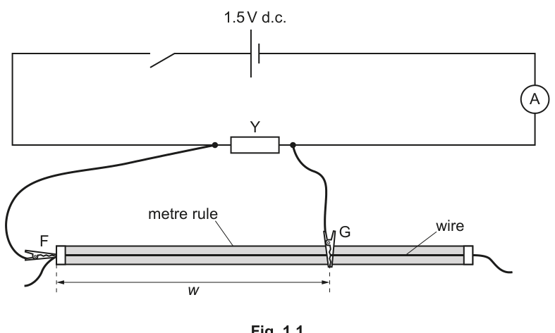
● F and G are crocodile clips.

The distance between F and G is $w$ . Attach G to the wire so that $w$ is approximately $70\text{ cm}$ .

● Close the switch.

● Record the value of $w$ and the ammeter reading $I_1$ .

$w$ = ______
$I_1$ = ______

● Open the switch.

DifficultyEasy

Worked solution

Answer

Record $w$ (to the nearest $1\ \text{mm}$ or $0.1\ \text{cm}$ ) and $I_1$ (to the ammeter resolution).

Example readings:

w = 70.0\ \text{cm}

I_1 = 0.39\ \text{A}

Final answer

Example: w = 70.0 cm, I1 = 0.39 A

Detailed explanation

Background Concept

In this practical you are measuring how current depends on the resistance of a length of wire. For a uniform wire, the resistance is proportional to its length:

R \propto w

When a fixed potential difference is applied, the current depends on the total resistance in the circuit:

I = \frac{V}{R_{\text{total}}}

So changing the length of wire between the crocodile clips changes the current.

Understanding the Question

You are told to:

set up the circuit exactly as in Fig. 1.1,
place crocodile clip G so the separation between F and G is about $70\ \text{cm}$ ,
close the switch and take two readings: the length $w$ and the current $I_1$ .

This part is assessed mainly on correct measurement and appropriate precision.

Approach

Attach F at the $0\ \text{cm}$ end of the wire on the metre rule.
Attach G near the $70\ \text{cm}$ mark (so $w \approx 70\ \text{cm}$ ).
Close the switch briefly and read the ammeter.
Open the switch to reduce heating of the wire.

Step-by-Step Reasoning

Measure $w$ as the distance along the scale from the contact point of F to the contact point of G.
Read the ammeter without parallax error (especially if analogue).
Record $w$ to metre-rule precision (typically $0.1\ \text{cm}$ ) and $I_1$ to the smallest scale division / display resolution of the ammeter.

Key Takeaways

Correctly identify what is being measured: a length on the wire and a current.
Record readings to sensible and consistent precision.
Minimise heating by keeping the switch closed only while taking a reading.

Common Mistakes

Measuring $w$ from the wrong end of the metre rule (not from F at the $0\ \text{cm}$ point).
Recording $w$ with no unit or unrealistic precision (e.g. many decimal places from a metre rule).
Leaving the switch closed for too long so the wire heats up and the current drifts.

Things to Be Careful About

Ensure the crocodile clip jaws make good electrical contact with the wire.
If the ammeter reading is unstable, wait briefly for it to settle, then record.
Keep the same definition of $w$ throughout (distance between the two clip contact points).

Techniques used

assemble a series electrical circuit from a circuit diagrammeasure a length on a metre rule between two clipsread an analogue or digital ammeter to appropriate precision

(b)

● Keep F and G in the same positions so that the value of $w$ remains the same.

● Change some of the connecting leads to set up the circuit shown in Fig. 1.2.

Fig. 1.2

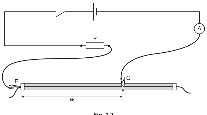
● Close the switch.

● Record the ammeter reading $I_2$ .

$I_2$ = ______

● Open the switch.

● Calculate $I_1 I_2$ .

$I_1 I_2$ = ______

DifficultyMedium-Easy

Worked solution

Working

Keep $w$ unchanged.

Example reading:

I_2 = 0.21\ \text{A}

Calculate:

I_1I_2 = (0.39)(0.21) = 0.0819\ \text{A}^2 \approx 0.082\ \text{A}^2

Answer

I_2 = 0.21\ \text{A}

I_1I_2 = 0.082\ \text{A}^2

Final answer

Example: I2 = 0.21 A, I1I2 = 0.082 A^2

Detailed explanation

Background Concept

This practical uses two current measurements, $I_1$ and $I_2$ , obtained from two different circuit connections but with the same wire length $w$ . You are then asked to calculate a derived quantity, the product $I_1I_2$ , which will later be used for graphing.

Derived quantities must be calculated using consistent units and then rounded appropriately.

Understanding the Question

You must:

keep F and G fixed so that $w$ stays the same,
rewire to match Fig. 1.2,
measure the new current $I_2$ ,
compute $I_1I_2$ using your $I_1$ from part (a).

Approach

Do not move the crocodile clips (so $w$ is controlled).
Only change leads necessary to make the circuit match Fig. 1.2.
Close the switch, read $I_2$ , then open the switch.
Multiply $I_1$ and $I_2$ to obtain $I_1I_2$ .

Step-by-Step Reasoning

Controlling $w$ is essential: the point is to see the effect of the new circuit arrangement, not a new wire length.
Take the ammeter reading $I_2$ with the same care as before (stable reading, correct precision).
Multiply:

I_1I_2 = I_1 \times I_2

Units: since both currents are in $\text{A}$ , the product has units $\text{A}^2$ .

Key Takeaways

When a question says “keep $w$ the same”, treat it as a control variable.
Always give units for calculated quantities.

Common Mistakes

Moving G accidentally so $w$ changes.
Forgetting that $I_1I_2$ has units $\text{A}^2$ .
Over-rounding early (round only at the end of the calculation).

Things to Be Careful About

Ensure the circuit really matches Fig. 1.2 (component placement matters).
State $I_2$ to the resolution of the ammeter; keep consistent decimal places across repeated readings later.

Techniques used

reconfigure a circuit by changing connecting leads while keeping a variable fixedrecord an ammeter reading to appropriate precisioncalculate a derived quantity by multiplying two measured values

(c)

Using values of $w$ greater than $55\text{ cm}$ , change $w$ by placing G at different positions on the wire and record $I_1$ and $I_2$ .

Repeat until you have six sets of readings of $w$ , $I_1$ and $I_2$ . Include your values from (a) and (b).

Record your results in a table. Include values of $I_1 I_2$ and $\frac{1}{w}$ in your table.

10M

DifficultyMedium-Hard

Worked solution

Answer

Take at least six sets of readings with $w > 55\ \text{cm}$ , each time recording $w$ , $I_1$ (Fig. 1.1 circuit) and $I_2$ (Fig. 1.2 circuit), then calculating $I_1I_2$ and $1/w$ .

Results table (single table) with headings including units, e.g.

$w / \text{cm}$	$I_1 / \text{A}$	$I_2 / \text{A}$	$I_1I_2 / \text{A}^2$	$1/w / \text{cm}^{-1}$
56.0	0.45	0.22	0.099	0.0179
60.0	0.42	0.22	0.093	0.0167
70.0	0.39	0.21	0.082	0.0143
75.0	0.37	0.21	0.078	0.0133
80.0	0.35	0.21	0.074	0.0125
90.0	0.32	0.21	0.067	0.0111

(Values shown are illustrative; your readings will differ.)

Final answer

Single results table with six sets of w, I1, I2 plus derived columns I1I2 and 1/w (with units).

Detailed explanation

Background Concept

Good experimental data needs:

a clear independent variable (here $w$ ),
enough values over a suitable range (here $w > 55\ \text{cm}$ , six readings),
consistent measurement technique,
a results table that includes both raw data and calculated quantities.

When you calculate new columns (like $I_1I_2$ and $1/w$ ), the accuracy and significant figures should be consistent with the raw measurements.

Understanding the Question

You must move clip G to create different values of $w$ (all greater than $55\ \text{cm}$ ). For each $w$ you need two currents:

$I_1$ from the Fig. 1.1 circuit,
$I_2$ from the Fig. 1.2 circuit,
and then you must calculate:

I_1I_2

and

\frac{1}{w}

Finally, all of this must appear in one clear table.

Approach

Choose six (or more) values of $w$ spread across the allowed range (e.g. from about $56\ \text{cm}$ up to near $95\text{–}100\ \text{cm}$ ).
For each $w$ $w$ :
- set up Fig. 1.1, measure $I_1$ ;
- without changing $w$ , rewire to Fig. 1.2, measure $I_2$ .
Calculate $I_1I_2$ and $1/w$ for each row.
Present all results in a single table with correct headings and consistent dp/s.f.

Step-by-Step Reasoning

Choosing the range: a wide range in $w$ gives a wider spread in $1/w$ , which makes the graph more reliable (a clearer straight-line trend).
Keeping conditions constant: do not change the power supply setting; ensure connections are firm; close the switch only when taking readings to reduce heating.
Repeats (good practice): if time allows, repeat a reading at one or more $w$ values to check consistency; if the current fluctuates, take repeat readings and use the mean.
Table headings: each column heading should be “quantity / unit”, e.g. $w / \text{cm}$ , not just “w”.
Calculated quantities:
- Multiply currents to get $I_1I_2$ in $\text{A}^2$ .
- Compute $1/w$ using the same unit of $w$ that you recorded (if $w$ is in cm, then $1/w$ is in $\text{cm}^{-1}$ ).
Precision: keep consistent decimal places for each column (e.g. all $w$ to 0.1 cm; all currents to 0.01 A; calculated values to 2–3 s.f.).

Key Takeaways

Collect enough data points over a meaningful range.
Control variables carefully (only $w$ should change between sets).
A good table has clear headings, units, consistent precision, and correctly calculated columns.

Common Mistakes

Using some $w$ values below $55\ \text{cm}$ (ignored by the instruction).
Splitting results into two tables (one for $I_1$ and one for $I_2$ ) instead of one combined table.
Missing units in column headings.
Inconsistent decimal places within a column.
Calculating $1/w$ using $w$ in cm for some rows and in m for others.

Things to Be Careful About

Do not round $I_1$ or $I_2$ before multiplying; use recorded values and round the product at the end.
If you change $w$ , you must measure both $I_1$ and $I_2$ for that same $w$ (don’t mix readings from different $w$ values).
Ensure crocodile clips make contact at the same reference points each time (contact point affects the true effective length).

Techniques used

vary an independent variable over a stated rangetake multiple sets of readings under controlled conditionscalculate derived columns from raw measurementspresent results in a single table with correct headings and units

(d)

(i)

Plot a graph of $I_1 I_2$ on the $y$ -axis against $\frac{1}{w}$ on the $x$ -axis.

DifficultyMedium

Worked solution

Answer

Plot a graph with:

$x$ -axis: $1/w$ (with unit from your table, e.g. $\text{cm}^{-1}$ ).
$y$ -axis: $I_1I_2$ (units $\text{A}^2$ ).

Use a sensible scale (at least half the grid on each axis) and plot all six points accurately as small crosses.

Final answer

Graph of I1I2 (y) against 1/w (x) plotted with correct labels/units and suitable scales.

Detailed explanation

Background Concept

Graphs in Paper 3 are assessed heavily on good plotting practice:

correct axes (right variables in the right places),
correct labels (quantity and unit),
scales that make best use of the paper,
points plotted accurately.

The goal is to see whether the relationship is linear.

Understanding the Question

You are told exactly what to plot:

vertical axis: $I_1I_2$ ,
horizontal axis: $1/w$ .

So you must use the two derived columns from your table.

Approach

Decide the axis ranges from your minimum and maximum values of $1/w$ and $I_1I_2$ .
Choose scales that are simple (e.g. 1 big square = 0.001, 0.002, 0.005, 0.01 etc.) and that use most of the grid.
Label each axis as “quantity / unit”.
Plot all points as neat crosses.

Step-by-Step Reasoning

Units: If your $w$ was in cm, then $1/w$ is in $\text{cm}^{-1}$ . If your $w$ was in m, then $1/w$ is in $\text{m}^{-1}$ . Your axis label must match your table.
Avoid awkward scales: scales like 3 squares = 0.01 are hard to use and lead to plotting errors.
Plotting: locate each value carefully; do not draw dots so large that you can’t tell the exact location.

Key Takeaways

A correct graph starts with correct labels and units.
Scale choice directly affects how accurately you can find gradients/intercepts later.

Common Mistakes

Swapping the axes (plotting $I_1I_2$ on $x$ and $1/w$ on $y$ ).
Missing units or writing units incorrectly (e.g. writing $1/w$ with unit cm).
Using a tiny portion of the grid (makes gradient uncertain).

Things to Be Careful About

Use the derived column values, not raw $w$ .
Keep consistent decimal places from the table when reading values.
If one point seems anomalous, still plot it; don’t discard points unless instructed.

Techniques used

choose suitable axes and scales that use most of the graph gridlabel axes with quantity and unitplot experimental points accurately from a results table

(ii)

Draw the straight line of best fit.

DifficultyMedium-Easy

Worked solution

Answer

Draw one straight line of best fit (not point-to-point), balanced so that the points are distributed roughly evenly above and below the line.

Final answer

Straight line of best fit drawn (balanced).

Detailed explanation

Background Concept

Experimental data usually show scatter due to random uncertainties. A line of best fit represents the underlying trend, not the random fluctuations.

For a relationship expected to be linear, you draw a straight line that best represents all points.

Understanding the Question

After plotting the points, you are asked to draw the straight line of best fit. This line will later be used to find the gradient and intercept.

Approach

Use a ruler.
Place the line so that the overall spread of points is balanced: roughly equal numbers (and similar scatter) above and below.
Do not force the line through every point.

Step-by-Step Reasoning

If one point is clearly off-trend, your best-fit line should still follow the majority trend.
Extend the line across the full range of the plotted data so you can read the intercept reliably.

Key Takeaways

A best-fit line summarises the trend in noisy data.
You need a good line to obtain an accurate gradient/intercept.

Common Mistakes

Joining the dots (creating a zig-zag line).
Forcing the line through the origin when it does not appear appropriate.
Drawing a line that follows an outlier rather than the main trend.

Things to Be Careful About

Use a sharp pencil for a thin line (thick lines make intercept readings uncertain).
Ensure the line covers the region where you will read the intercept (often near $x=0$ ).

Techniques used

judge whether data are consistent with a straight line trenddraw a balanced best-fit straight line through scattered pointsavoid joining point-to-point when a trend line is required

(iii)

Determine the gradient and $y$ -intercept of this line.

gradient = ______
$y$ -intercept = ______

DifficultyMedium

Worked solution

Working

Use two well-separated points on the best-fit line.

Example (from a large triangle):

\text{gradient} = \frac{\Delta (I_1I_2)}{\Delta (1/w)}

\text{gradient} = 5.0\ \text{A}^2\,\text{cm}

Read the $y$ -intercept at $1/w = 0$ :

\text{$y$-intercept} = 0.010\ \text{A}^2

Answer

\text{gradient} = 5.0\ \text{A}^2\,\text{cm}

\text{$y$-intercept} = 0.010\ \text{A}^2

(Values shown are illustrative; use your graph readings.)

Final answer

Student-dependent; example gradient = 5.0 A^2 cm, y-intercept = 0.010 A^2

Detailed explanation

Background Concept

For a straight-line graph,

y = mx + c

where:

$m$ is the gradient (slope),
$c$ is the $y$ -intercept (value of $y$ when $x=0$ ).

On a plotted graph, the most accurate way to find the gradient is to use a large triangle on the best-fit line (not between two experimental points).

Understanding the Question

You must obtain two numerical values from your best-fit straight line:

the gradient,
the $y$ -intercept.

Here:

$y = I_1I_2$ (units $\text{A}^2$ )
$x = 1/w$ (units depend on how you measured $w$ ; e.g. $\text{cm}^{-1}$ )

Approach

Pick two points far apart on the best-fit line (preferably at grid intersections).
Read their coordinates $(x_1,y_1)$ and $(x_2,y_2)$ .
Compute:

m = \frac{y_2-y_1}{x_2-x_1}

Find the $y$ -intercept by extending the best-fit line to $x=0$ and reading $y$ .

Step-by-Step Reasoning

grad-triangle

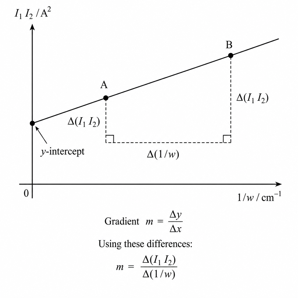
Large triangle: the bigger the triangle, the smaller the percentage reading error in $\Delta x$ and $\Delta y$ .
Gradient units:

[m] = \frac{\text{A}^2}{\text{cm}^{-1}} = \text{A}^2\,\text{cm}

(if $x$ is in $\text{cm}^{-1}$ ). If you used $\text{m}^{-1}$ then the gradient unit becomes $\text{A}^2\,\text{m}$ .

Intercept units: the intercept is a value of $I_1I_2$ , so it always has units $\text{A}^2$ .

Key Takeaways

Use the best-fit line, not individual data points, for gradient.
Use a large triangle to reduce uncertainty.
Always quote gradient and intercept with units.

Common Mistakes

Using two adjacent points (small triangle \u2192 large uncertainty).
Calculating $\Delta x/\Delta y$ instead of $\Delta y/\Delta x$ .
Forgetting to include units or giving incorrect units for the gradient.
Reading the intercept from the wrong place (it is at $x=0$ , not at the first data point).

Things to Be Careful About

Choose points that lie exactly on the best-fit line and are easy to read (grid intersections).
Keep sign correct: if the line slopes upward, gradient is positive.
Extend the line neatly to $x=0$ with a ruler to read the intercept accurately.

Techniques used

use a large triangle on a best-fit line to calculate gradientcalculate gradient as \u0394y/\u0394x with unitsread y-intercept at x = 0 from the best-fit line

(e)

It is suggested that the quantities $I_1$ , $I_2$ and $w$ are related by the equation

I_1 I_2 = \frac{P}{w} + Q

where $P$ and $Q$ are constants.

Using your answers in (d)(iii), determine values for $P$ and $Q$ . Give appropriate units.

$P$ = ______
$Q$ = ______

DifficultyMedium-Easy

Worked solution

Working

Given:

I_1I_2 = \frac{P}{w} + Q

Let $y = I_1I_2$ and $x = 1/w$ . Then:

y = Px + Q

So:

P = \text{gradient}, \qquad Q = \text{$y$-intercept}

Using the example values from (d)(iii):

P = 5.0\ \text{A}^2\,\text{cm}

Q = 0.010\ \text{A}^2

Answer

P = 5.0\ \text{A}^2\,\text{cm}

Q = 0.010\ \text{A}^2

(Use your own gradient and intercept; if $1/w$ was in $\text{m}^{-1}$ then $P$ is in $\text{A}^2\,\text{m}$ .)

Final answer

P = gradient, Q = y-intercept (with appropriate units).

Detailed explanation

Background Concept

Many practical relationships are tested by plotting a graph that should be a straight line. If you can rewrite the suggested equation into the form:

y = mx + c

then you can identify constants directly:

gradient $m$ corresponds to a constant,
intercept $c$ corresponds to another constant.

Understanding the Question

You are given:

I_1I_2 = \frac{P}{w} + Q

and you have already plotted $I_1I_2$ against $1/w$ and found the gradient and intercept. You must now use those two graph values to determine $P$ and $Q$ , including units.

Approach

Identify the variables on your graph:
- $y = I_1I_2$
- $x = 1/w$
Rewrite the equation in terms of $x$ :

I_1I_2 = P\left(\frac{1}{w}\right) + Q

Compare with $y = mx + c$ to match constants.
Use axis units to assign units to $P$ and $Q$ .

Step-by-Step Reasoning

Let $x = 1/w$ . Then:

I_1I_2 = Px + Q

Comparing with $y = mx + c$ :

P = m, \qquad Q = c

Units:

$Q$ is a value of $I_1I_2$ , so:

[Q] = \text{A}^2

$P$ has units of gradient:

[P] = \frac{\text{units of } I_1I_2}{\text{units of } (1/w)}

If $1/w$ is in $\text{cm}^{-1}$ , then:

[P] = \frac{\text{A}^2}{\text{cm}^{-1}} = \text{A}^2\,\text{cm}

If $1/w$ is in $\text{m}^{-1}$ , then $[P] = \text{A}^2\,\text{m}$ .

Key Takeaways

Converting to $y = mx + c$ lets you read constants from gradient and intercept.
Units come directly from the axis units.

Common Mistakes

Stating $P$ has units $\text{A}^2$ (forgetting it comes from the gradient).
Mixing cm and m between table, graph, and final units.
Swapping $P$ and $Q$ .

Things to Be Careful About

Your value of $P$ depends on the unit used for $w$ (cm vs m). Always keep it consistent with the graph you actually drew.
Quote $P$ and $Q$ to a sensible number of significant figures based on how well you could read the gradient/intercept from your graph.

Techniques used

match an experimental linear graph to the form y = mx + cidentify physical constants from gradient and interceptdetermine units of constants from axis units

The rest of this paper

1 more questions

Q2Manipulation, Measurement and Observation · Analysis, Conclusions and Evaluation · Presentation of Data and Observations20M

Loading the full paper…