Physics 9702/35 — October/November 2022

Cambridge AS Level · Advanced Practical Skills · worked solutions for every part, with the mark scheme

questions

marks

120

minutes

Topics Manipulation, Measurement and Observation · Presentation of Data and Observations · Analysis, Conclusions and Evaluation

Q120MManipulation, Measurement and ObservationPresentation of Data and ObservationsAnalysis, Conclusions and EvaluationFree sample

In this experiment, you will investigate the balancing of a metre rule.

(a)

● Set up the apparatus as shown in Fig. 1.1.

Fig. 1.1

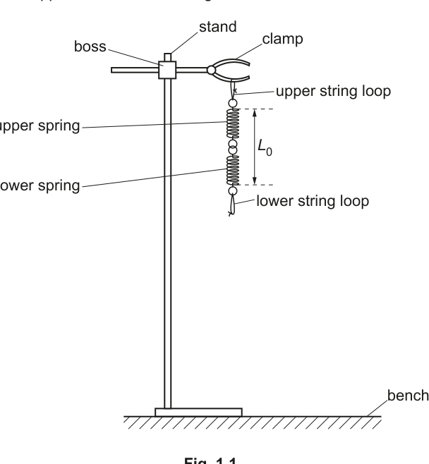
● The length $L_0$ of the spring combination is measured between the top coil of the upper spring and the bottom coil of the lower spring, as shown in Fig. 1.1.

Measure and record $L_0$ .

$L_0$ = ______ $\text{cm}$

● Use the lower string loop to suspend a total mass of $200\text{ g}$ , as shown in Fig. 1.2.

Fig. 1.2

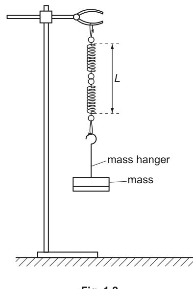
● The new length of the spring combination is $L$ .

Measure and record $L$ .

$L$ = ______ $\text{cm}$

● The spring constant $k$ of the spring combination is given by the equation

k = \frac{W}{(L - L_0)}

where $W$ is $1.96\text{ N}$ .

Calculate $k$ .

DifficultyMedium-Easy

Worked solution

Working

(Example readings)

$L_0 = 18.0\ \text{cm}$

With $200\ \text{g}$ :

$L = 23.0\ \text{cm}$

L-L_0 = (23.0-18.0)\ \text{cm} = 5.0\ \text{cm} = 0.050\ \text{m}

k = \frac{W}{(L-L_0)} = \frac{1.96}{0.050} = 39.2\ \text{N m}^{-1}

Answer

$k = 39.2\ \text{N m}^{-1}$

Final answer

k = 39.2 N m^-1

Detailed explanation

Background Concept

For a spring (or spring combination) obeying Hooke’s law, the force (weight) and extension are related by

F = kx

where:

$F$ is the applied force (here the weight $W$ in newtons),
$x$ is the extension (change in length) in metres,
$k$ is the spring constant in $\text{N m}^{-1}$ .

Rearranging gives:

k = \frac{F}{x}

Understanding the Question

You measure the unstretched length of the two-spring combination ( $L_0$ ) and then the stretched length ( $L$ ) when a total mass of $200\ \text{g}$ is hung. The extension is $L-L_0$ .

You are told to use

k = \frac{W}{(L-L_0)}

with $W = 1.96\ \text{N}$ , and you must calculate $k$ .

Approach

Measure $L_0$ and $L$ to the same precision (typically to the nearest $0.1\ \text{cm}$ ).
Find the extension $L-L_0$ .
Convert the extension from $\text{cm}$ to $\text{m}$ so that $k$ comes out in $\text{N m}^{-1}$ .
Substitute into the given equation.

Step-by-Step Reasoning

Using representative readings (your own readings will differ):

Suppose $L_0 = 18.0\ \text{cm}$ .
With $200\ \text{g}$ added, suppose $L = 23.0\ \text{cm}$ .

Then the extension is

L-L_0 = 23.0-18.0 = 5.0\ \text{cm}

Convert to metres:

5.0\ \text{cm} = 5.0 \times 10^{-2}\ \text{m} = 0.050\ \text{m}

Now substitute into the given formula:

k = \frac{1.96}{0.050} = 39.2\ \text{N m}^{-1}

Key Takeaways

Extension is a difference of two measured lengths.
Always use SI units in Hooke’s law calculations unless you intentionally use consistent non-SI units.
Quoting $k$ with correct units is essential.

Common Mistakes

Using $L$ instead of $L-L_0$ (forgetting to calculate extension).
Not converting $\text{cm}$ to $\text{m}$ , giving a value of $k$ too small by a factor of $100$ .
Writing incorrect units (e.g. $\text{N cm}^{-1}$ when the calculation used metres).

Things to Be Careful About

Read lengths without parallax (eye level with scale).
Use consistent precision: if lengths are read to $0.1\ \text{cm}$ , the extension should be reported accordingly.
Ensure the springs hang vertically so the length measured is the true extension.

Techniques used

take length readings to an appropriate precision from a scalecalculate an extension from two length measurementsconvert centimetres to metres for use in an SI equationsubstitute into an equation to determine a constant

(b)

● Set up the apparatus as shown in Fig. 1.3.

Fig. 1.3

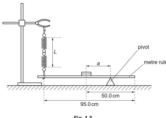
● Use the adhesive putty to fix two $100\text{ g}$ slotted masses with their centres above the $50.0\text{ cm}$ mark on the rule. The masses must remain at this position throughout the experiment.

● Place the lower string loop at the $5.0\text{ cm}$ mark on the rule.

● The distance between the pivot and the midpoint of the rule is $a$ .

Adjust the pivot so that $a$ is approximately $25\text{ cm}$ .

● Adjust the stand, boss and clamp so that the springs are vertical and the rule is horizontal.

● Measure and record $a$ and $L$ .

$a$ = ______
$L$ = ______

● The extension of the spring combination is given by the equation

e = L - L_0

Calculate $e$ .

$e$ = ______

● Change $a$ by moving the pivot. Adjust the stand, boss and clamp so that the springs are vertical and the rule is horizontal. Measure $a$ and $L$ . Repeat until you have six sets of values of $a$ and $L$ .
Do not include values of $a$ less than $15.0\text{ cm}$ .

Record your results in a table. Include values of $e$ , $\frac{1}{a}$ and $\frac{1}{e}$ in your table.

DifficultyMedium

Worked solution

Working

(Using $L_0 = 18.0\ \text{cm}$ from (a); example data shown.)

e = L-L_0

Example (first row):

e = 22.6-18.0 = 4.6\ \text{cm}

Reciprocals in $\text{m}^{-1}$ (convert $\text{cm}\to\text{m}$ ):

\frac{1}{a} = \frac{1}{a/100} = \frac{100}{a\ (\text{cm})} \qquad \frac{1}{e} = \frac{100}{e\ (\text{cm})}

Answer

(Example table format and values)

$a / \text{cm}$	$L / \text{cm}$	$e / \text{cm}$	$\frac{1}{a} / \text{m}^{-1}$	$\frac{1}{e} / \text{m}^{-1}$
15.0	22.6	4.6	6.67	21.7
18.0	22.9	4.9	5.56	20.4
22.0	23.3	5.3	4.55	18.9
26.0	23.6	5.6	3.85	17.9
30.0	23.9	5.9	3.33	16.9
35.0	24.1	6.1	2.86	16.4

Final answer

See working (student-dependent table of a, L, e, 1/a, 1/e)

Detailed explanation

Background Concept

In Paper 3 you are rewarded for:

taking a sensible range of readings for the independent variable,
repeating measurements to improve reliability,
recording data clearly in a single table,
calculating derived quantities correctly and consistently.

Here the required derived quantities are:

e = L-L_0

and the reciprocals $\frac{1}{a}$ and $\frac{1}{e}$ to allow a straight-line graph later.

Understanding the Question

You set up the metre rule balanced by a pivot and supported by a spring combination. You then:

choose different positions of the pivot so that $a$ changes (but keep $a \ge 15.0\ \text{cm}$ ),
each time, re-adjust so the springs are vertical and the rule is horizontal,
measure $a$ and the new spring length $L$ ,
calculate the extension $e$ using $L_0$ from (a),
calculate $1/a$ and $1/e$ and record everything in one table.

Approach

Decide what to vary: vary $a$ by moving the pivot position.
Keep control variables fixed: the two $100\ \text{g}$ masses stay at $50.0\ \text{cm}$ ; the spring attachment stays at $5.0\ \text{cm}$ .
For each pivot position:
- ensure equilibrium (rule horizontal; springs vertical),
- record $a$ and $L$ with consistent precision,
- calculate $e=L-L_0$ .
Add calculated columns $1/a$ and $1/e$ .

Step-by-Step Reasoning

Measure $a$ as the distance between the pivot and the midpoint of the rule (the $50.0\ \text{cm}$ mark). Record to the nearest $0.1\ \text{cm}$ if the scale allows.
Measure $L$ (length of the spring combination) to the nearest $0.1\ \text{cm}$ .

Calculate extension for each reading:

e = L-L_0

Example: if $L=22.6\ \text{cm}$ and $L_0=18.0\ \text{cm}$ ,

e = 22.6-18.0 = 4.6\ \text{cm}

Now calculate reciprocals. You can either:

keep everything in $\text{cm}$ and use $\text{cm}^{-1}$ , or
convert to SI and use $\text{m}^{-1}$ .

A neat method to get $\text{m}^{-1}$ directly from centimetres is:

\frac{1}{a} = \frac{1}{a/100} = \frac{100}{a\ (\text{cm})}

and similarly

\frac{1}{e} = \frac{100}{e\ (\text{cm})}

Then record all values in one clear table with headings like $a/\text{cm}$ , $L/\text{cm}$ , $e/\text{cm}$ , $1/a\,/\text{m}^{-1}$ , $1/e\,/\text{m}^{-1}$ .

Key Takeaways

Collect at least six sets of readings across a good range of $a$ .
Ensure the system is in equilibrium before reading $a$ and $L$ .
A good results table has: quantity + unit in the heading, and consistent significant figures down each column.

Common Mistakes

Using values of $a<15.0\ \text{cm}$ (explicitly disallowed).
Not keeping the two $100\ \text{g}$ masses fixed at the $50.0\ \text{cm}$ mark.
Calculating $e$ incorrectly (e.g. $L_0-L$ or mixing cm and m).
Missing units in headings, or spreading results across multiple tables.

Things to Be Careful About

Read $a$ carefully: it is a distance between pivot and the midpoint (not the pivot reading itself).
Use consistent decimal places for $a$ , $L$ , and therefore $e$ .
When taking reciprocals, do not round too early; calculate using the measured value then round sensibly.

Techniques used

adjust the pivot position to vary an independent variable over a suitable rangemeasure distances and lengths consistently to a stated precisioncalculate derived quantities from raw readingscompute reciprocal values for linearisationrecord results in a well-structured table with correct headings and units

(c)

(i)

Plot a graph of $\frac{1}{e}$ on the $y$ -axis against $\frac{1}{a}$ on the $x$ -axis.

DifficultyMedium-Easy

Worked solution

Answer

Plot $\dfrac{1}{e}$ (unit $\text{m}^{-1}$ ) on the $y$ -axis against $\dfrac{1}{a}$ (unit $\text{m}^{-1}$ ) on the $x$ -axis using the six data points from the table.

Final answer

Graph of 1/e (y) against 1/a (x) plotted

Detailed explanation

Background Concept

A graph is used to test whether two quantities are related linearly. If the expected relationship is

y = mx + c

then plotting $y$ against $x$ should give a straight line.

Good graph technique in Cambridge practicals includes:

correct axis labels (quantity and unit),
sensible scales (not cramped; not awkward like 3 squares = 1 unit),
accurate plotting.

Understanding the Question

You have calculated $\frac{1}{a}$ and $\frac{1}{e}$ in your table. This part tells you exactly what to plot:

vertical axis: $\frac{1}{e}$ ,
horizontal axis: $\frac{1}{a}$ .

Approach

Draw axes and label them clearly with units.
Choose scales so the plotted data fill at least half the grid in both directions.
Plot each of the six points with small, neat crosses.

Step-by-Step Reasoning

Take each row of your results table.
Read $x = 1/a$ and $y = 1/e$ .
Mark the point at $(x,y)$ .

Axis labels should be written as, for example:

$x$ -axis: $\frac{1}{a} / \text{m}^{-1}$
$y$ -axis: $\frac{1}{e} / \text{m}^{-1}$

(If you used $\text{cm}^{-1}$ , then state $\text{cm}^{-1}$ consistently on both axes.)

Key Takeaways

Put the independent variable on the $x$ -axis.
Always include units.
Use sensible scales and plot accurately.

Common Mistakes

Swapping axes (plotting $1/a$ on $y$ by mistake).
Missing units in axis labels.
Using a scale that wastes most of the graph paper.

Things to Be Careful About

If you rounded reciprocal values heavily, points may scatter more; keep enough significant figures in the table.
Plot from the table values, not from intermediate rounded numbers on a calculator screen.

Techniques used

choose axes so the independent variable is on the x-axislabel axes with quantity and unitselect a scale that uses a large fraction of the graph gridplot points accurately from a results table

(ii)

Draw the straight line of best fit.

DifficultyEasy

Worked solution

Answer

Draw a single straight line of best fit through the plotted points (not dot-to-dot).

Final answer

Straight best-fit line drawn

Detailed explanation

Background Concept

A best-fit line represents the overall trend in the data. In experimental data there is scatter due to random uncertainties, so the line should pass as close as possible to all points, with roughly equal scatter above and below.

Understanding the Question

After plotting the points in (c)(i), you are asked to draw the straight line that best represents them.

Approach

Use a ruler to draw one straight line that:

follows the trend,
has about the same number of points above and below,
does not join points one by one.

Step-by-Step Reasoning

Place a ruler so that it visually balances the scatter.
Adjust until the line is a good compromise.
Draw the line across the full extent of the data region (not just between two middle points).

Key Takeaways

Best fit means “balances” the scatter, not necessarily passing through every point.

Common Mistakes

Dot-to-dot joining of points.
Forcing the line through the origin when not required.

Things to Be Careful About

Do not make the line too thick; it should be thin and precise so gradient/intercept readings are accurate.

Techniques used

draw a single straight line that balances the scatter of pointsignore minor anomalies when fitting a best-fit line

(iii)

Determine the gradient and $y$ -intercept of this line.

gradient = ______
$y$ -intercept = ______

DifficultyMedium

Worked solution

Working

(Example from a typical best-fit line.)

Choose two points on the best-fit line, e.g.
$(x_1,y_1) = (2.86,16.4)$ and $(x_2,y_2) = (6.67,21.7)$ where $x=\dfrac{1}{a}$ and $y=\dfrac{1}{e}$ in $\text{m}^{-1}$ .

\text{gradient} = \frac{\Delta y}{\Delta x} = \frac{21.7-16.4}{6.67-2.86} = \frac{5.3}{3.81} = 1.39

$y$ -intercept from the line at $x=0$ :

y\text{-intercept} = 12.4\ \text{m}^{-1}

Answer

gradient $= 1.39$

$y$ -intercept $= 12.4\ \text{m}^{-1}$

Final answer

gradient = 1.39; y-intercept = 12.4 m^-1

Detailed explanation

Background Concept

For a straight-line graph,

y = mx + c

the gradient is $m = \frac{\Delta y}{\Delta x}$ ,
the $y$ -intercept is $c$ (the value of $y$ when $x=0$ ).

On a graph you should calculate the gradient using a large triangle on the best-fit line to reduce percentage reading uncertainty.

Understanding the Question

You have plotted $y = 1/e$ against $x = 1/a$ and drawn a best-fit straight line. Now you must:

find the gradient of that line,
find where it crosses the $y$ -axis.

Approach

Pick two points on the best-fit line (not necessarily measured points) that are far apart.
Read their coordinates carefully.
Compute $m = \Delta y / \Delta x$ .
Extend the line to $x=0$ and read off $c$ .

Step-by-Step Reasoning

Suppose you read two well-separated points on the drawn best-fit line, such as:
- $(x_1,y_1)=(2.86,16.4)$
- $(x_2,y_2)=(6.67,21.7)$

Compute the changes:

\Delta y = 21.7-16.4 = 5.3\ \text{m}^{-1}

\Delta x = 6.67-2.86 = 3.81\ \text{m}^{-1}

So the gradient is

m = \frac{\Delta y}{\Delta x} = \frac{5.3}{3.81} = 1.39

Notice the units cancel: $(\text{m}^{-1})/(\text{m}^{-1})$ so the gradient is dimensionless.

To find the $y$ -intercept, extend the best-fit line back to where it meets the $y$ -axis (at $x=0$ ) and read off that value. In this example, it is $12.4\ \text{m}^{-1}$ .

Key Takeaways

Use a large triangle for the gradient.
Use points on the best-fit line rather than noisy raw data points.
Check units: the intercept has the same unit as $y$ .

Common Mistakes

Using $\Delta x/\Delta y$ instead of $\Delta y/\Delta x$ .
Choosing two points very close together, giving a large percentage uncertainty.
Taking coordinates from plotted points that are not on the best-fit line.

Things to Be Careful About

Read coordinates to a sensible precision consistent with your graph scale.
If the line does not actually reach the $y$ -axis on the paper, extend it with a ruler before reading the intercept.

Techniques used

select two well-separated points on the best-fit linecalculate a gradient using \Delta y / \Delta xread the y-intercept from a graph at x = 0

(d)

(i)

It is suggested that the quantities $e$ and $a$ are related by the equation

\frac{1}{e} = B \frac{1}{a} + C

where $B$ and $C$ are constants.

Using your answers in (c)(iii), determine the values of $B$ and $C$ . Give appropriate units.

$B$ = ______
$C$ = ______

DifficultyMedium-Easy

Worked solution

Working

Given

\frac{1}{e} = B\frac{1}{a} + C

Comparing with $y = mx + c$ for the graph of $y=\dfrac{1}{e}$ against $x=\dfrac{1}{a}$ :

B = \text{gradient},\qquad C = y\text{-intercept}

Using (c)(iii):

B = 1.39\ (\text{no unit})

C = 12.4\ \text{m}^{-1}

Answer

$B = 1.39$

$C = 12.4\ \text{m}^{-1}$

Final answer

B = 1.39 (no unit); C = 12.4 m^-1

Detailed explanation

Background Concept

When a graph is plotted as $y$ against $x$ and produces a straight line, it can be compared to

y = mx + c

gradient $m$ corresponds to the coefficient of $x$ ,
intercept $c$ corresponds to the constant term.

Units:

The gradient has units of (units of $y$ )/(units of $x$ ).
The intercept has units of $y$ .

Understanding the Question

You are told the suggested relationship is

\frac{1}{e} = B\frac{1}{a} + C

and you have already found the gradient and $y$ -intercept from your graph in (c)(iii). You must identify $B$ and $C$ and give units.

Approach

Treat the equation as $y = mx + c$ with:

$y = 1/e$ ,
$x = 1/a$ .
Then read off:
$B$ from the gradient,
$C$ from the intercept.

Step-by-Step Reasoning

Comparing

\frac{1}{e} = B\frac{1}{a} + C

with

y = mx + c

gives:

B = m,\qquad C = c

If both axes are in $\text{m}^{-1}$ , then:

gradient $B$ has units $(\text{m}^{-1})/(\text{m}^{-1})$ so it is dimensionless,
intercept $C$ has units $\text{m}^{-1}$ .

So, using the example values from (c)(iii), $B=1.39$ and $C=12.4\ \text{m}^{-1}$ .

Key Takeaways

Constants in a linear relationship come directly from gradient and intercept.
Unit checking is a quick way to catch mistakes.

Common Mistakes

Giving a unit for $B$ when both axes have the same unit (it should cancel).
Mixing $\text{cm}^{-1}$ and $\text{m}^{-1}$ between table/graph and later calculations.

Things to Be Careful About

If you used $\text{cm}^{-1}$ on the graph, then $C$ would be in $\text{cm}^{-1}$ and you must stay consistent later (or convert).

Techniques used

match a straight-line equation to y = mx + cidentify constants from the gradient and interceptdeduce units from axis units

(ii)

Theory suggests that

C = \frac{k}{(R + W)}

where $R$ is the weight of the rule and $W$ is $1.96\text{ N}$ .

Using your answers in (a) and (d)(i), determine a value for $R$ .

$R$ = ______ $\text{N}$

DifficultyMedium

Worked solution

Working

Given

C = \frac{k}{(R+W)}

Rearrange:

R+W = \frac{k}{C} qquad\Rightarrow\qquad R = \frac{k}{C} - W

Using $k = 39.2\ \text{N m}^{-1}$ from (a), $C = 12.4\ \text{m}^{-1}$ from (d)(i), and $W=1.96\ \text{N}$ :

R = \frac{39.2}{12.4} - 1.96 = 3.16 - 1.96 = 1.20\ \text{N}

Answer

$R = 1.20\ \text{N}$

Final answer

R = 1.20 N

Detailed explanation

Background Concept

A theoretical model often links a graph constant (like an intercept) to physical parameters. Here,

C = \frac{k}{(R+W)}

relates:

$C$ (from the graph of $1/e$ against $1/a$ ),
$k$ (spring constant from part (a)),
$R$ (weight of the metre rule),
$W$ (known hanging weight, here $1.96\ \text{N}$ ).

Dimensional check:

$k$ has unit $\text{N m}^{-1}$ ,
$(R+W)$ has unit $\text{N}$ ,
so $k/(R+W)$ has unit $\text{m}^{-1}$ , matching the unit of $C$ .

Understanding the Question

You must use your experimentally determined $k$ and $C$ to calculate the rule’s weight $R$ .

Approach

Rearrange the given equation to make $R$ the subject.
Substitute values of $k$ , $C$ , and $W$ .
Ensure units are consistent (especially $C$ in $\text{m}^{-1}$ if $k$ is in $\text{N m}^{-1}$ ).

Step-by-Step Reasoning

Start with:

C = \frac{k}{(R+W)}

Multiply both sides by $(R+W)$ :

C(R+W) = k

Divide by $C$ :

R+W = \frac{k}{C}

Subtract $W$ :

R = \frac{k}{C} - W

Now substitute example experimental values:

$k = 39.2\ \text{N m}^{-1}$ ,
$C = 12.4\ \text{m}^{-1}$ ,
$W = 1.96\ \text{N}$ .

Then:

R = \frac{39.2}{12.4} - 1.96 = 3.16 - 1.96 = 1.20\ \text{N}

The value is reasonable: $R=1.20\ \text{N}$ corresponds to a mass of about $0.122\ \text{kg}$ .

Key Takeaways

Use intercept/gradient values as experimentally determined constants.
Always check unit consistency before substituting.
Rearrangement accuracy is crucial for 1-mark calculations.

Common Mistakes

Using $C$ in $\text{cm}^{-1}$ together with $k$ in $\text{N m}^{-1}$ (unit mismatch).
Rearranging incorrectly (e.g. $R = kC - W$ ).
Forgetting to subtract $W$ to isolate $R$ .

Things to Be Careful About

If your graph used $\text{cm}^{-1}$ , convert $C$ to $\text{m}^{-1}$ by multiplying by $100$ before using it with $k$ in $\text{N m}^{-1}$ .
Quote $R$ with an appropriate number of significant figures consistent with $k$ and $C$ .

Techniques used

rearrange an equation to make an unknown the subjectsubstitute experimental constants into a theoretical relationshipcheck dimensional consistency and quote an answer with units

The rest of this paper

1 more questions

Q2Manipulation, Measurement and Observation · Analysis, Conclusions and Evaluation · Presentation of Data and Observations20M

Loading the full paper…