Physics 9702/33 — October/November 2022

Cambridge AS Level · Advanced Practical Skills · worked solutions for every part, with the mark scheme

questions

marks

120

minutes

Topics Manipulation, Measurement and Observation · Presentation of Data and Observations · Analysis, Conclusions and Evaluation

Q1Manipulation, Measurement and ObservationPresentation of Data and ObservationsAnalysis, Conclusions and EvaluationFree sample

In this experiment, you will determine the resistivity of a metal.

(a)

● Set up the circuit shown in Fig. 1.1.

Fig. 1.1

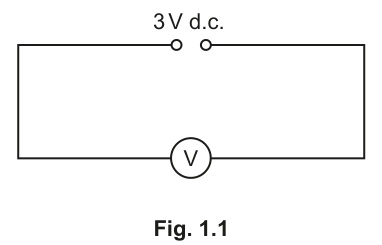
● Record the voltmeter reading $E$ .

$E$ = ______ $\text{V}$

● Set up the circuit shown in Fig. 1.2.

Fig. 1.2

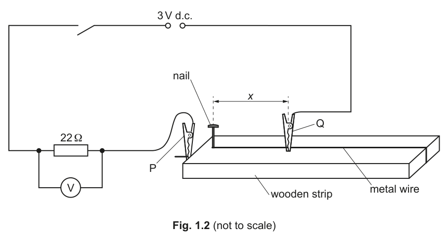
● P and Q are crocodile clips.

The distance between the nail and Q is $x$ , as shown in Fig. 1.2.

Adjust the position of Q until $x$ is approximately $45\text{ cm}$ .

● Close the switch.

● The voltmeter reading is $V$ .

Measure and record $x$ and $V$ .

$x$ = ______
$V$ = ______

● Open the switch.

DifficultyMedium-Easy

Worked solution

Answer

Record voltmeter readings to an appropriate precision (e.g. $0.01\ \text{V}$ ) and measure $x$ to the nearest $\text{mm}$ .

Example recorded values:

$E = 3.00\ \text{V}$

$x = 45.0\ \text{cm}$

$V = 1.35\ \text{V}$

Final answer

E = 3.00 V, x = 45.0 cm, V = 1.35 V (example readings)

Detailed explanation

Background Concept

In this experiment you vary the effective length $x$ of a metal wire in a circuit and measure a potential difference $V$ using a voltmeter. A voltmeter measures the potential difference between two points in a circuit and should be connected in parallel with the component (or section of circuit) whose p.d. is required.

When taking practical readings, marks are often awarded for:

using the apparatus correctly (e.g. correct circuit connections),
choosing an appropriate range (here $x \approx 45\ \text{cm}$ initially),
recording measurements to a sensible precision (linked to instrument resolution).

Understanding the Question

You are instructed to:

Set up Fig. 1.1 and record the supply/reference voltmeter reading $E$ .
Set up Fig. 1.2 with crocodile clips $P$ and $Q$ , adjust $Q$ so that the distance from the nail to $Q$ is about $45\ \text{cm}$ , then close the switch and record $x$ and the voltmeter reading $V$ .

The numbers are not given in the paper because they depend on your own apparatus and how you set it up.

Approach

Build each circuit exactly as shown.
For each required reading: close the switch briefly, wait for the reading to settle, then record it.
Measure $x$ from the stated reference point (the nail) to the position of clip $Q$ .
Record $E$ and $V$ with a precision consistent with the voltmeter scale (typically $0.01\ \text{V}$ for a digital meter).

Step-by-Step Reasoning

Measure $E$ (Fig. 1.1): connect the voltmeter as in the diagram, close the circuit, and record the steady reading. A typical value for a nominal $3\ \text{V}$ supply could be around $3.00\ \text{V}$ .
Set $x \approx 45\ \text{cm}$ (Fig. 1.2): place crocodile clip $Q$ along the wire and use a ruler/metre rule to measure the distance from the nail to $Q$ . Record $x$ (e.g. $45.0\ \text{cm}$ ).
Measure $V$ (Fig. 1.2): close the switch, allow the voltmeter reading to stabilise, then record $V$ (e.g. $1.35\ \text{V}$ ). Open the switch after taking the reading to reduce heating of the wire.

Key Takeaways

Record voltmeter readings to an appropriate decimal place.
Measure $x$ from the correct reference point and record units.
Keep the switch closed only long enough to take a reading to reduce temperature changes.

Common Mistakes

Measuring $x$ from the wrong end of the wire (not from the nail).
Leaving the switch closed continuously, causing heating and changing resistance.
Recording voltmeter readings with inconsistent precision (e.g. mixing $1.3\ \text{V}$ and $1.35\ \text{V}$ ).

Things to Be Careful About

Ensure good contact with crocodile clips; poor contact adds extra resistance and makes readings unstable.
Read $x$ perpendicular to the scale to reduce parallax (especially with a ruler/metre rule).
Check that the voltmeter is on the correct range so it does not overload and so it gives adequate resolution.

Techniques used

set up the circuit according to the diagramtake a voltmeter reading with the switch closedmeasure a length along the wire from a defined reference point

(b)

Change $x$ by adjusting the position of Q on the wire. Use six different values of $x$ . For each value of $x$ , measure $V$ .

Record your results in a table. Include values of $\frac{1}{V}$ in your table.

DifficultyMedium

Worked solution

Answer

Record six pairs of $x$ and $V$ readings, and calculate $\dfrac{1}{V}$ for each.

Example results table (your values will differ):

$x\ /\ \text{cm}$	$V\ /\ \text{V}$	$1/V\ /\ \text{V}^{-1}$
$20.0$	$1.06$	$0.943$
$30.0$	$1.16$	$0.862$
$40.0$	$1.28$	$0.781$
$45.0$	$1.35$	$0.741$
$55.0$	$1.52$	$0.658$
$65.0$	$1.72$	$0.581$

Final answer

Table of six x and V values with a calculated 1/V column (see working).

Detailed explanation

Background Concept

In Paper 3, marks for a results table are awarded for good scientific presentation:

a single table containing all relevant data,
clear column headings with quantity and unit (e.g. $x/\text{cm}$ ),
consistent decimal places/significant figures within each column,
correct calculation of any derived quantity (here $1/V$ ).

$V$ is a measured voltage; $1/V$ is a calculated quantity whose unit is $\text{V}^{-1}$ .

Understanding the Question

You must:

vary $x$ by moving crocodile clip $Q$ ,
use six different values of $x$ ,
measure the corresponding voltmeter reading $V$ for each,
record the data in a table, including a third column for $1/V$ .

Approach

Choose a sensible range of $x$ values (spread out, not clustered), ensuring the circuit still works and readings remain stable.
For each $x$ , close the switch briefly, record $V$ , then open the switch.
Compute $1/V$ for each row using the recorded $V$ .
Present in a single table with headings and units.

Step-by-Step Reasoning

Decide on six $x$ values (e.g. from about $20\ \text{cm}$ to $65\ \text{cm}$ ) to provide a wide spread for graphing.
For each row:
- measure $x$ with a ruler/metre rule (typically to $\pm 0.1\ \text{cm}$ or better),
- record $V$ from the voltmeter (e.g. to $\pm 0.01\ \text{V}$ if digital),
- calculate $1/V$ using a calculator.

Example calculation for one row:

\frac{1}{V} = \frac{1}{1.35\ \text{V}} = 0.741\ \text{V}^{-1}

Note how the calculated values are given to a consistent number of significant figures (commonly 3 s.f.), because they come from measured values.

Key Takeaways

Use six well-spaced $x$ values to improve the reliability of the graph.
Always include units in headings, not in every cell.
Derived quantities must be calculated correctly and consistently.

Common Mistakes

Missing units in the headings (e.g. writing just $x$ and $V$ ).
Writing $1/V$ but giving the wrong unit (it must be $\text{V}^{-1}$ ).
Inconsistent precision (e.g. $x=20, 30.0, 40.00$ in the same column).
Using too narrow a range of $x$ , leading to a poor graph.

Things to Be Careful About

Avoid values of $x$ that make $V$ very small or very close to the supply value (readings can become less reliable).
If the voltmeter reading drifts, check clip contact and avoid heating (open the switch between readings).
Ensure $1/V$ is calculated from the displayed $V$ values (do not round $V$ too early).

Techniques used

collect readings over a suitable range of the independent variablerecord results in a table with correct headings and unitscalculate a derived quantity for each readinguse consistent significant figures within each column

(c)

(i)

Plot a graph of $\frac{1}{V}$ on the $y$ -axis against $x$ on the $x$ -axis.

DifficultyMedium

Worked solution

Answer

Plot a graph with:

$y$ -axis labelled $1/V\ (\text{V}^{-1})$
$x$ -axis labelled $x\ (\text{cm})$
a suitable scale using at least half the grid in each direction
all six points plotted accurately.

Final answer

Graph of 1/V (V^-1) against x (cm) plotted.

Detailed explanation

Background Concept

A graph is used to test whether two quantities have a linear relationship. Good graphing technique is assessed by:

correct axes (independent variable on $x$ -axis, dependent on $y$ -axis),
clear labels with units,
sensible scales (not cramped, not awkward like 3 squares = 1 unit),
accurate plotting.

Understanding the Question

You are told to plot $\dfrac{1}{V}$ on the $y$ -axis against $x$ on the $x$ -axis using your table from (b). This is a direct instruction about what to put on each axis.

Approach

Use your calculated $1/V$ values as the vertical coordinates.
Use your measured $x$ values as the horizontal coordinates.
Choose scales that make your plotted points spread out.

Step-by-Step Reasoning

Draw axes and mark a clear origin (it does not have to be $(0,0)$ if your data does not include values near zero; you can start at e.g. $x = 15\ \text{cm}$ if needed).
Label axes:
- horizontal: $x/\text{cm}$ ,
- vertical: $1/V\ /\ \text{V}^{-1}$ .
Choose scales so points occupy most of the available grid.
Plot each of the six points as small, neat crosses (not blobs).

Key Takeaways

Axis labels must include units.
A good scale improves gradient accuracy later.
Plotting accuracy directly affects the gradient and intercept you calculate.

Common Mistakes

Swapping axes (plotting $x$ on the $y$ -axis).
Writing units incorrectly (e.g. $1/V$ in $\text{V}$ instead of $\text{V}^{-1}$ ).
Using a scale that compresses points into a small area.

Things to Be Careful About

Plot with a sharp pencil; use a ruler for reading coordinates.
Do not force the line through the origin unless the data strongly supports it (that comes in part (ii)).

Techniques used

choose suitable axis scales that use most of the graph gridlabel axes with quantity and unitplot points accurately from a results table

(ii)

Draw the straight line of best fit.

DifficultyMedium-Easy

Worked solution

Answer

Draw a single straight line of best fit with approximately equal scatter of points above and below the line.

Final answer

Straight line of best fit drawn.

Detailed explanation

Background Concept

A best-fit line represents the overall trend in the data. Because experimental data contains random errors, points do not usually lie exactly on a straight line even if the relationship is linear.

Understanding the Question

After plotting the points in (c)(i), you must draw the straight line that best represents them.

Approach

Use a ruler.
Place the line so that the vertical deviations of points are balanced: roughly as many points above as below.
Do not join point-to-point; it must be one straight line.

Step-by-Step Reasoning

Visually judge the trend of the plotted points.
Use a ruler to draw a straight line through the middle of the scatter.
Ensure the line extends across the range of plotted points (not just between two central points).

Key Takeaways

A best-fit line is not the same as connecting data points.
Balance of scatter is the key criterion.

Common Mistakes

Drawing a zig-zag line joining points.
Forcing the line through the origin without justification.
Drawing a line that passes through an outlier but misses most points.

Things to Be Careful About

If one point is clearly an outlier (obvious mistake), you may still draw the best-fit line for the main trend, but do not simply ignore multiple points.

Techniques used

draw a straight line of best fit balancing points above and belowignore minor scatter consistent with experimental uncertainty

(iii)

Determine the gradient and $y$ -intercept of this line.

gradient = ______
$y$ -intercept = ______

DifficultyMedium

Worked solution

Working

Using two points on the best-fit line, e.g.
$(x,\ 1/V) = (20.0\ \text{cm},\ 0.943\ \text{V}^{-1})$ and $(65.0\ \text{cm},\ 0.581\ \text{V}^{-1})$ :

\text{gradient} = \frac{\Delta (1/V)}{\Delta x} = \frac{0.581 - 0.943}{65.0 - 20.0} = -8.04 \times 10^{-3}\ \text{V}^{-1}\ \text{cm}^{-1}

\text{y-intercept} = c = (1/V) - (\text{gradient})x = 0.943 - (-8.04 \times 10^{-3})(20.0) = 1.10\ \text{V}^{-1}

Answer

gradient $= -8.0 \times 10^{-3}\ \text{V}^{-1}\ \text{cm}^{-1}$

y-intercept $= 1.10\ \text{V}^{-1}$

Final answer

gradient = -8.0×10^-3 V^-1 cm^-1, y-intercept = 1.10 V^-1 (example)

Detailed explanation

Background Concept

For a straight-line graph,

y = mx + c

$m$ is the gradient (slope), found from $\Delta y / \Delta x$ .
$c$ is the $y$ -intercept, the value of $y$ when $x=0$ (read from where the line crosses the $y$ -axis).

In practical work, you should use points on the best-fit line, not necessarily the raw plotted points.

Understanding the Question

You must determine the gradient and the $y$ -intercept of your line on the graph of $1/V$ (vertical axis) against $x$ (horizontal axis). The values depend on your data.

Approach

Pick two points far apart on the best-fit line (to reduce percentage uncertainty).
Read off their coordinates carefully.
Compute gradient as:

\text{gradient} = \frac{(1/V)_2 - (1/V)_1}{x_2 - x_1}

Find the intercept by reading it from the graph or by substituting one point into $y = mx + c$ .

Step-by-Step Reasoning

Choose two well-separated points (often near the ends of the line). Using points too close together makes $\Delta x$ small and the gradient very sensitive to reading error.
Calculate the gradient with correct order: change in $y$ divided by change in $x$ .
Units: since $y$ is in $\text{V}^{-1}$ and $x$ is in $\text{cm}$ , gradient has units $\text{V}^{-1}\ \text{cm}^{-1}$ .
For the intercept, either:
- extend the line to the $y$ -axis and read the crossing value, or
- use $c = y - mx$ with one chosen point.

Key Takeaways

Use points on the drawn line, far apart.
Gradient is $\Delta y/\Delta x$ , not $y/x$ .
Always include units for gradient and intercept.

Common Mistakes

Using two plotted points that are not on the best-fit line.
Using $\Delta x/\Delta y$ (inverting the gradient).
Giving gradient with incorrect units (or no units).

Things to Be Careful About

If the line is decreasing, gradient must be negative.
Read coordinates with the same precision that the graph grid allows (typically to half a small square).

Techniques used

select two well-separated points on the best-fit linecalculate gradient using $\Delta y/\Delta x$determine the y-intercept from the line

(d)

It is suggested that the quantities $V$ and $x$ are related by the equation

\frac{1}{V} = Ax + B

where $A$ and $B$ are constants.

Using your answers in (c)(iii), determine the values of $A$ and $B$ . Give appropriate units.

$A$ = ______
$B$ = ______

DifficultyMedium-Easy

Worked solution

Answer

Comparing

\frac{1}{V} = Ax + B

with $y = mx + c$ :

A = \text{gradient} = -8.0 \times 10^{-3}\ \text{V}^{-1}\ \text{cm}^{-1}

B = \text{y-intercept} = 1.10\ \text{V}^{-1}

Final answer

A = -8.0×10^-3 V^-1 cm^-1, B = 1.10 V^-1 (example)

Detailed explanation

Background Concept

If a graph is plotted with $y$ against $x$ and the relationship is

y = mx + c,

then:

$m$ is the gradient of the line,
$c$ is the $y$ -intercept.

Here the equation is already in straight-line form:

\frac{1}{V} = Ax + B.

So $A$ plays the role of gradient, and $B$ plays the role of intercept.

Understanding the Question

You are asked to use your graph results from (c)(iii) to find $A$ and $B$ and to give their units.

Approach

Identify $A$ as the gradient you calculated.
Identify $B$ as the intercept you calculated/read.
Determine units from the plotted quantities: $1/V$ has units $\text{V}^{-1}$ and $x$ has units of length (e.g. cm).

Step-by-Step Reasoning

Since $1/V$ is on the $y$ -axis, $y$ has units $\text{V}^{-1}$ .
Since $x$ is on the $x$ -axis (in cm in the example), $x$ has units $\text{cm}$ .
Therefore the gradient $A$ has units:

\frac{\text{V}^{-1}}{\text{cm}} = \text{V}^{-1}\ \text{cm}^{-1}.

The intercept $B$ has the same units as $y$ , i.e. $\text{V}^{-1}$ .

Key Takeaways

When the equation matches $y = mx + c$ , constants map directly to gradient and intercept.
Units come from axis units, not from the symbols alone.

Common Mistakes

Giving $A$ the wrong sign (it must match the slope direction).
Forgetting units or giving $A$ in $\text{V}^{-1}$ instead of $\text{V}^{-1}\ \text{cm}^{-1}$ .

Things to Be Careful About

If you plotted $x$ in $\text{m}$ instead of $\text{cm}$ , then $A$ must be in $\text{V}^{-1}\ \text{m}^{-1}$ . Be consistent with your own graph.

Techniques used

match a straight-line graph to y = mx + cidentify constants from gradient and interceptstate units from the plotted axis units

(e)

(i)

Use a micrometer to measure the diameter $d$ of the wire.

$d$ = ______

DifficultyMedium-Easy

Worked solution

Answer

Measure $d$ with a micrometer (check zero error) and take several readings along the wire.

Example mean diameter:

d = 0.32\ \text{mm}

Final answer

d = 0.32 mm (example mean)

Detailed explanation

Background Concept

A micrometer screw gauge is used for small diameters and typically has a resolution of $0.01\ \text{mm}$ (or $0.001\ \text{mm}$ for some digital micrometers). Good technique includes:

checking for zero error,
gently tightening using the ratchet (to apply consistent force),
taking repeated measurements and averaging.

Understanding the Question

You must measure the wire diameter $d$ and record it. This diameter will later be used to calculate cross-sectional area and hence resistivity, so it is an important measurement.

Approach

Check the micrometer reads $0.00\ \text{mm}$ when fully closed (or note any zero error).
Take diameter readings at several different positions along the wire and rotate the wire slightly to check for non-circularity.
Average the readings and record $d$ to the micrometer resolution.

Step-by-Step Reasoning

Close the micrometer gently using the ratchet; note any zero error.
Place the wire between anvil and spindle; tighten with the ratchet until it clicks.
Read the main scale and thimble scale (or read directly if digital).
Repeat at least 3 times at different points.
Compute the mean and apply any zero correction.

Key Takeaways

Micrometer measurements should be repeated.
Diameter is usually the largest source of uncertainty in resistivity experiments because area depends on $d^2$ .

Common Mistakes

Not using the ratchet, leading to inconsistent compression and readings.
Forgetting to correct for a non-zero reading when closed.
Recording too many decimal places not justified by the instrument.

Things to Be Careful About

Do not squash soft wire: excessive force gives a smaller diameter.
Ensure the wire is perpendicular to the micrometer faces (no tilt).

Techniques used

use a micrometer correctly including zero checktake repeated measurements at different positionscalculate a mean diameter and quote appropriate precision

(ii)

It is suggested that $A$ is given by the equation

A = -\frac{4\rho}{\pi d^2 ER}

where $R$ is $22\Omega$ and $\rho$ is the resistivity of the metal.

Using your answers in (a), (d) and (e)(i), determine a value for $\rho$ . Give an appropriate unit.

$\rho$ = ______

DifficultyMedium-Hard

Worked solution

Working

Given

A = -\frac{4\rho}{\pi d^2 E R}

\rho = -\frac{A\pi d^2 E R}{4}

Convert $A$ to $\text{V}^{-1}\ \text{m}^{-1}$ (if gradient was in $\text{cm}^{-1}$ ):

A = -8.0 \times 10^{-3}\ \text{V}^{-1}\ \text{cm}^{-1} = -0.80\ \text{V}^{-1}\ \text{m}^{-1}

Using $d = 0.32\ \text{mm} = 3.2 \times 10^{-4}\ \text{m}$ , $E = 3.00\ \text{V}$ and $R = 22\ \Omega$ :

\rho = -\frac{(-0.80)\pi(3.2 \times 10^{-4})^2(3.00)(22)}{4}

\rho = 4.2 \times 10^{-6}\ \Omega\ \text{m}

Answer

$\rho = 4.2 \times 10^{-6}\ \Omega\ \text{m}$

Final answer

ρ = 4.2×10^-6 Ω m (example)

Detailed explanation

Background Concept

Resistivity $\rho$ is a material property defined (for a uniform wire) by

R_{\text{wire}} = \rho\frac{L}{A}

where $L$ is length and $A$ is cross-sectional area. In this experiment the analysis leads to a linear relationship

\frac{1}{V} = Ax + B

and the constant $A$ is related to $\rho$ via the given formula:

A = -\frac{4\rho}{\pi d^2 E R}.

Here $d$ determines the area $A_{\text{cs}} = \pi d^2/4$ , so small errors in $d$ strongly affect $\rho$ .

Understanding the Question

You must use your measured/derived values:

$E$ from (a),
$A$ from (d),
$d$ from (e)(i),

and the known $R = 22\ \Omega$ to calculate $\rho$ .

The key practical subtlety is unit consistency: $\rho$ should end up in $\Omega\ \text{m}$ , so all lengths must be in metres.

Approach

Rearrange the given equation to make $\rho$ the subject.
Convert all measurements to SI units:
- $d$ in metres,
- if your gradient $A$ used $x$ in cm, convert $A$ to per metre.
Substitute values and compute $\rho$ .
Quote $\rho$ with an appropriate unit and sensible significant figures.

Step-by-Step Reasoning

Rearrange for $\rho$ :

A = -\frac{4\rho}{\pi d^2 E R} \quad\Rightarrow\quad \rho = -\frac{A\pi d^2 E R}{4}.

Convert units:

Diameter: if $d = 0.32\ \text{mm}$ ,

d = 0.32\ \text{mm} = 0.32 \times 10^{-3}\ \text{m} = 3.2 \times 10^{-4}\ \text{m}.

Gradient: if your graph used $x$ in cm, then $A$ is in $\text{V}^{-1}\ \text{cm}^{-1}$ . Since

1\ \text{cm}^{-1} = 100\ \text{m}^{-1},

you multiply by 100 to convert to per metre:

-8.0 \times 10^{-3}\ \text{V}^{-1}\ \text{cm}^{-1} = -0.80\ \text{V}^{-1}\ \text{m}^{-1}.

Substitute values:

\rho = -\frac{(-0.80)\pi(3.2 \times 10^{-4})^2(3.00)(22)}{4}.

Interpret sign and unit: $A$ is negative, so the two negatives cancel, giving a positive resistivity (as expected). The correct unit is $\Omega\ \text{m}$ .

Key Takeaways

Always convert to SI units before substituting into formulas for physical constants.
If $x$ was in cm on the graph, the gradient must be converted to per metre for use in SI equations.
Resistivity should be a positive value with unit $\Omega\ \text{m}$ .

Common Mistakes

Using $A$ in $\text{V}^{-1}\ \text{cm}^{-1}$ directly without converting to $\text{m}^{-1}$ .
Using $d$ in mm instead of m.
Dropping the minus sign and obtaining a negative $\rho$ .

Things to Be Careful About

Significant figures: $d$ is often only to 2 s.f., so $\rho$ should not be over-precise.
Squaring $d$ : keep enough digits during the calculation to avoid rounding error.
Ensure you use the measured $E$ from Fig. 1.1 (not just the nominal value of the supply).

Techniques used

rearrange a given equation to make the required variable the subjectconvert measured quantities into consistent SI unitssubstitute measured values with correct significant figurescheck units of the final derived quantity

The rest of this paper

1 more questions

Q2Manipulation, Measurement and Observation · Analysis, Conclusions and Evaluation · Presentation of Data and Observations20M

Loading the full paper…