Physics 9702/34 — May/June 2022

Cambridge AS Level · Advanced Practical Skills · worked solutions for every part, with the mark scheme

questions

marks

120

minutes

Topics Manipulation, Measurement and Observation · Presentation of Data and Observations · Analysis, Conclusions and Evaluation

Q1Manipulation, Measurement and ObservationPresentation of Data and ObservationsAnalysis, Conclusions and EvaluationFree sample

In this experiment you will investigate an electrical circuit.

(a)

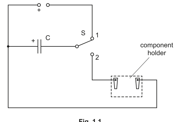
You have been provided with the circuit shown in Fig. 1.1.

Fig. 1.1

● Connect the voltmeter in parallel with component C, as shown in Fig. 1.2.

Fig. 1.2

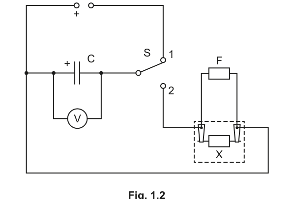
● Connect the resistor labelled F in parallel with the component holder, as shown in Fig. 1.2.
● Connect one of the labelled resistors into the component holder as resistor X, as shown in Fig. 1.2. Record the resistance $R$ of resistor X.

$R$ = ______

● Switch on the power supply.
● Move S to position 1.
● Record the voltmeter reading $V$ .

$V$ = ______

DifficultyEasy

Worked solution

Answer

Example readings (student-dependent):

$R = 100\ \Omega$

$V = 2.50\ \text{V}$

Final answer

See working (student-dependent readings)

Detailed explanation

Background Concept

A voltmeter measures the potential difference (p.d.) between two points in a circuit. It must be connected in parallel with the component because it compares the potentials at the two ends of that component.

Resistors may be combined in series or parallel. In this task you are instructed to place a resistor $F$ in parallel with the component holder, and a chosen resistor $X$ in the holder.

Understanding the Question

You are given a circuit containing a capacitor $C$ and a two-way switch $S$ . You must:

connect the voltmeter across the capacitor (parallel with $C$ ),
connect resistor $F$ in parallel with the holder,
insert resistor $X$ into the holder,
record the resistance $R$ of $X$ (from its label/value),
with $S$ at position 1, record the capacitor p.d. $V$ .

The numerical values depend on the particular resistors and supply provided.

Approach

Make the required parallel connections (voltmeter across $C$ , resistor $F$ across the holder).
Insert one labelled resistor as $X$ and note its stated resistance $R$ .
Set $S$ to position 1, allow the voltmeter reading to settle, then record $V$ with unit.

Step-by-Step Reasoning

The voltmeter must go across the capacitor terminals, so the meter reads the p.d. across $C$ directly.
The resistor value $R$ is recorded with unit $\Omega$ (typically as given on the resistor label).
With the supply switched on and $S$ at position 1, the capacitor charges; when the reading is steady, record $V$ in volts.

Key Takeaways

Voltmeters are always connected in parallel.
Record readings with correct units and sensible precision.

Common Mistakes

Connecting the voltmeter in series (gives incorrect operation and readings).
Writing the resistor value without units.
Recording a fluctuating voltmeter reading before it settles at $S$ position 1.

Things to Be Careful About

Ensure the voltmeter range is suitable to avoid over-range.
Check that connections are secure; loose leads cause unstable readings.
Record exactly what is asked: $R$ for resistor $X$ and the voltmeter reading $V$ at position 1.

Techniques used

connect a voltmeter in parallel with a componentidentify and record a resistor value with appropriate unittake a steady voltmeter reading at a specified switch position

(b)

● Ensure S is at position 1.
● Move S to position 2 and start the stop-watch. The voltmeter reading will gradually decrease.
● Stop the stop-watch when the voltmeter reading passes $0.8\ \text{V}$ .
● Record the time $t$ shown by the stop-watch.

$t$ = ______

● Move S to position 1.

DifficultyMedium-Easy

Worked solution

Answer

Example reading (student-dependent):

$t = 10.0\ \text{s}$

Final answer

See working (student-dependent reading)

Detailed explanation

Background Concept

When the switch is moved so that the charged capacitor is connected to a resistive path, the capacitor discharges and its p.d. decreases with time. The voltmeter reading therefore falls gradually.

A stopwatch measurement of a time interval should be taken using a clear start event and a clear stop event.

Understanding the Question

With $S$ initially at position 1, you then move $S$ to position 2 and start timing immediately. You stop timing when the voltmeter reading passes $0.8\ \text{V}$ . You must record the corresponding time $t$ .

Approach

Make sure the capacitor starts from the same initial condition each time by putting $S$ back to position 1 before repeating.
Start the stopwatch at the instant you move $S$ to position 2.
Watch the voltmeter and stop the stopwatch as the reading goes through $0.8\ \text{V}$ .

Step-by-Step Reasoning

Set $S$ to position 1 so the capacitor is charged (consistent starting p.d.).
Move $S$ to position 2 and start the stopwatch at the same instant.
Observe the voltmeter reading decreasing.
Stop the stopwatch at the moment the reading goes from above $0.8\ \text{V}$ to below $0.8\ \text{V}$ (i.e. it passes $0.8\ \text{V}$ ).
Record $t$ with unit $\text{s}$ and to the stopwatch resolution (often $0.1\ \text{s}$ ).
Return $S$ to position 1 to reset for the next run.

Key Takeaways

Use consistent start/stop definitions for timing.
Resetting the circuit between runs improves repeatability.

Common Mistakes

Stopping the timer when the reading is exactly $0.8\ \text{V}$ (may never be exactly displayed); the instruction is “passes $0.8\ \text{V}$ ”.
Forgetting to reset to position 1 before the next measurement.
Recording $t$ with no unit.

Things to Be Careful About

Reaction time is a significant uncertainty here; try to anticipate the moment the reading crosses $0.8\ \text{V}$ .
Keep your eye level with the analogue scale (if analogue) to reduce parallax.
Ensure the voltmeter reading is not oscillating due to poor connections.

Techniques used

synchronise switching with starting a stopwatchidentify the moment a voltmeter reading passes a specified valuerecord time to appropriate resolution

(c)

Change X and repeat (b) until you have six sets of values of $R$ and $t$ .

Record your results in a table. Include values of $\frac{1}{R}$ and $\frac{1}{t}$ in your table.

DifficultyMedium

Worked solution

Answer

A single table with 6 sets of values of $R$ and $t$ , including calculated $\dfrac{1}{R}$ and $\dfrac{1}{t}$ .

Example (values are student-dependent):

$R / \Omega$	$t / \text{s}$	$1/R / \Omega^{-1}$	$1/t / \text{s}^{-1}$
$47$	$5.3$	$0.0213$	$0.189$
$68$	$7.3$	$0.0147$	$0.137$
$100$	$10.0$	$0.0100$	$0.100$
$150$	$13.6$	$0.00667$	$0.0735$
$220$	$17.7$	$0.00455$	$0.0565$
$330$	$22.6$	$0.00303$	$0.0442$

Final answer

See working (table of 6 readings with 1/R and 1/t)

Detailed explanation

Background Concept

In practical work, you must record raw measurements clearly and then calculate any derived quantities accurately.

For a graph of $\dfrac{1}{t}$ against $\dfrac{1}{R}$ , it is helpful to treat $R$ as the independent variable (you choose different resistors) and $t$ as the dependent variable (you measure the time response). The reciprocal columns $1/R$ and $1/t$ are calculated from the measured values.

Understanding the Question

You must change resistor $X$ and repeat the timing procedure until you have six pairs of values $(R, t)$ . Then you must present the results in a table that also includes:

$\dfrac{1}{R}$ for each resistor,
$\dfrac{1}{t}$ for each timing.

Approach

Choose six different resistors $X$ with a good spread of $R$ values.
For each resistor: record $R$ , measure $t$ (using the method in part (b)).
Calculate $1/R$ and $1/t$ for each row.
Present all results in one neat table with correct headings (quantity and unit) and consistent numerical precision.

Step-by-Step Reasoning

Choosing the range: Pick resistors that are not all similar (e.g. from tens of ohms up to a few hundred ohms) so your graph has a good spread of $1/R$ values.
Recording $R$ : Use the labelled value (or measure with a multimeter if instructed) and write it with unit $\Omega$ .
Measuring $t$ : Time until the voltmeter reading passes $0.8\ \text{V}$ ; record in seconds, usually to $0.1\ \text{s}$ .
Calculating reciprocals:
- If $R = 100\ \Omega$ , then $\frac{1}{R} = \frac{1}{100\ \Omega} = 0.0100\ \Omega^{-1}.$
- If $t = 10.0\ \text{s}$ , then $\frac{1}{t} = \frac{1}{10.0\ \text{s}} = 0.100\ \text{s}^{-1}.$
Presentation: Keep decimal places consistent down each calculated column (or use consistent significant figures, commonly 3 s.f. for reciprocals). Ensure the table is not split into multiple small tables.

Key Takeaways

A good table has clear headings with units, consistent formatting, and all required derived quantities.
A wide range of data helps produce a reliable best-fit line later.

Common Mistakes

Missing units in headings (e.g. writing just $R$ instead of $R/\Omega$ ).
Calculating $1/R$ or $1/t$ with inconsistent rounding (random different s.f. each row).
Providing fewer than six sets of readings.

Things to Be Careful About

Do not round too early: calculate using full calculator precision, then round the final displayed reciprocal.
Make sure $\Omega^{-1}$ and $\text{s}^{-1}$ are used correctly for reciprocal units.
If you repeat timings, be consistent in how you average (state if you averaged); otherwise use a single careful timing each run as instructed.

Techniques used

collect multiple pairs of readings while varying one componentconstruct a results table with headings and unitscalculate reciprocal quantities with consistent significant figureschoose a suitable range of the independent variable

(d)

(i)

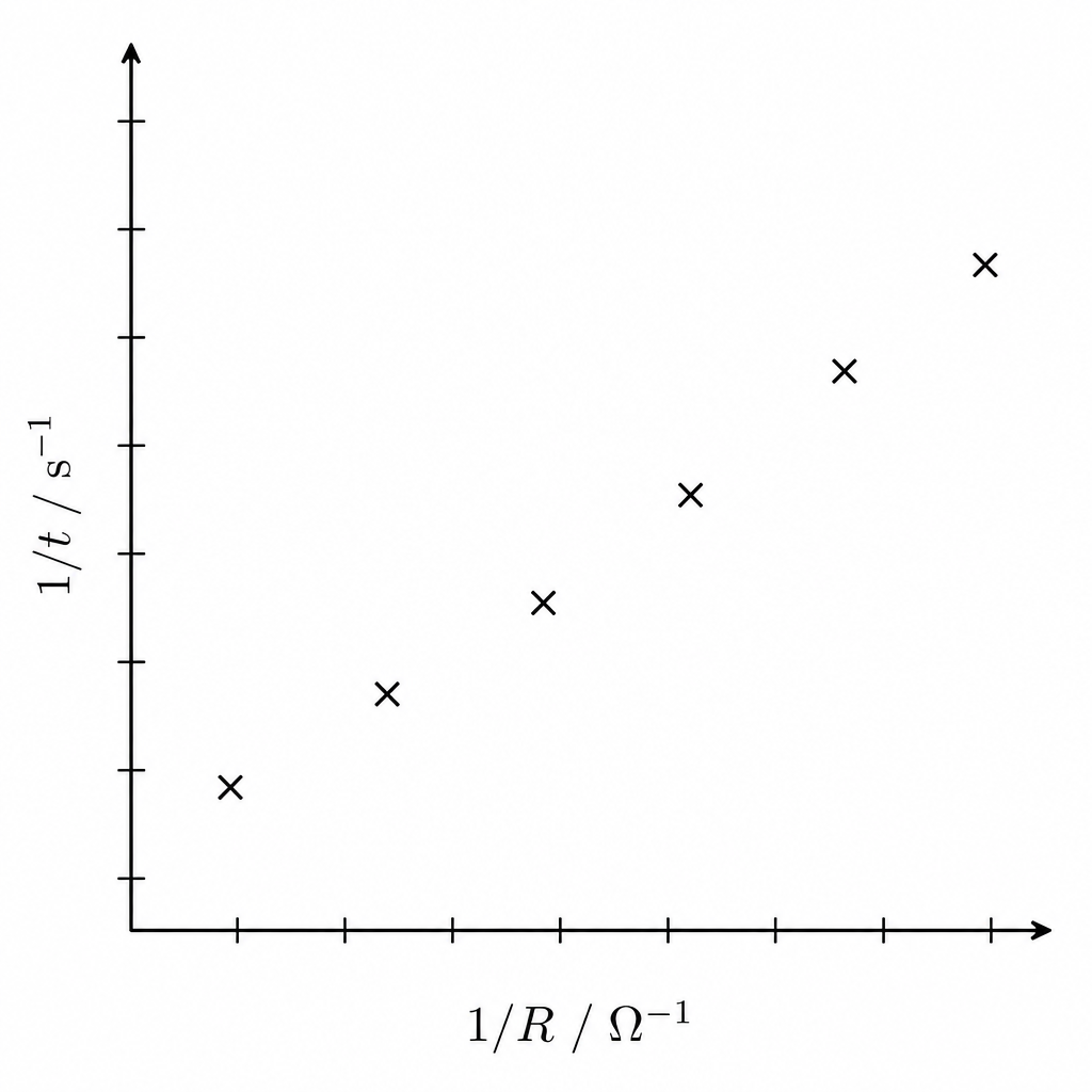
Plot a graph of $\frac{1}{t}$ on the $y$ -axis against $\frac{1}{R}$ on the $x$ -axis.

DifficultyMedium-Easy

Worked solution

Answer

Plot a graph with:

$x$ -axis: $1/R\ /\ \Omega^{-1}$
$y$ -axis: $1/t\ /\ \text{s}^{-1}$

Plot all six data points accurately using a suitable scale.

Final answer

Graph of 1/t (y) against 1/R (x)

Detailed explanation

Background Concept

A graph is used to reveal whether two quantities have a linear relationship. If a relationship has the form

\frac{1}{t} = \frac{a}{R} + b,

then plotting $y = 1/t$ against $x = 1/R$ should produce a straight line.

Understanding the Question

You have already calculated columns of $1/R$ and $1/t$ . You are now asked to plot:

$1/t$ on the vertical axis (the $y$ -axis),
$1/R$ on the horizontal axis (the $x$ -axis).

Approach

Draw axes covering a large area of the graph paper.
Label each axis with the correct quantity and unit.
Choose scales that use at least half of the available grid in both directions.
Plot each point as a small cross at the correct coordinates.

Step-by-Step Reasoning

Decide the range of $1/R$ and $1/t$ from your table (minimum to maximum).
Pick scales such that the points spread out well (avoid scales like 3 squares = 0.01 unless it is necessary).
Label axes, for example:
- horizontal: $1/R\ /\ \Omega^{-1}$
- vertical: $1/t\ /\ \text{s}^{-1}$
Plot all six points carefully (sharp pencil, fine crosses).

graph-axes

Key Takeaways

Correct axes and good scales are essential for accurate gradients.
Units must be included on graph axes.

Common Mistakes

Swapping axes (plotting $1/R$ on $y$ and $1/t$ on $x$ ).
Missing units or writing units incorrectly.
Using a tiny portion of the graph paper so the best-fit line and gradient are unreliable.

Things to Be Careful About

Plot from the calculated columns ( $1/R$ and $1/t$ ), not from $R$ and $t$ .
Use consistent precision when reading coordinates (typically to half a small square).
Do not join the points dot-to-dot; you will draw a best-fit line in the next part.

Techniques used

label axes with quantity and unitchoose a suitable linear scale using most of the gridplot points accurately from a table

(ii)

Draw the straight line of best fit.

DifficultyEasy

Worked solution

Answer

Draw one straight line of best fit through the plotted points (balanced about the line).

Final answer

Straight line of best fit drawn

Detailed explanation

Background Concept

If the experimental relationship is linear, the plotted points should lie close to a straight line. Because of measurement uncertainty, points will not lie exactly on the line; the best-fit line represents the underlying trend.

Understanding the Question

You must draw the straight line that best represents all the plotted data points on your $1/t$ vs $1/R$ graph.

Approach

Use a ruler.
Draw a single straight line.
Aim for roughly equal scatter of points above and below the line.
Do not force the line through every point.

Step-by-Step Reasoning

Place the ruler so that the line passes as close as possible to all points overall.
Check that no single outlier is dominating the fit.
Extend the line across most of the graph width so that gradient and intercept can be read accurately.

Key Takeaways

Best-fit means “overall trend”, not “connect the dots”.

Common Mistakes

Joining points dot-to-dot.
Drawing a line forced through the origin when the data do not support it.
Drawing a line that goes only through the middle points and ignores the ends.

Things to Be Careful About

If you have an obvious outlier, still draw the best-fit line based on the main trend unless instructed otherwise.
A thin pencil line improves the accuracy of later gradient/intercept measurements.

Techniques used

draw a single straight line that balances scatteravoid joining points dot-to-dotextend the best-fit line across the plotted range

(iii)

Determine the gradient and $y$ -intercept of this line.

gradient = ______
$y$ -intercept = ______

DifficultyMedium

Worked solution

Working

Using two well-separated points on the best-fit line, for example:

(x_1,y_1) = (0.0200\ \Omega^{-1},\ 0.180\ \text{s}^{-1}),\quad (x_2,y_2) = (0.00500\ \Omega^{-1},\ 0.0600\ \text{s}^{-1})

\text{gradient} = \frac{\Delta y}{\Delta x} = \frac{0.180-0.0600}{0.0200-0.00500} = 8.0\ \Omega\ \text{s}^{-1}

$y$ -intercept (from graph):

y\text{-intercept} = 0.020\ \text{s}^{-1}

Answer

gradient $= 8.0\ \Omega\ \text{s}^{-1}$

$y$ -intercept $= 0.020\ \text{s}^{-1}$

Final answer

gradient = 8.0 Ω s^-1, y-intercept = 0.020 s^-1 (example)

Detailed explanation

Background Concept

For a straight-line graph,

y = mx + c,

$m$ is the gradient (slope): $m = \frac{\Delta y}{\Delta x}$
$c$ is the $y$ -intercept: the value of $y$ when $x = 0$ .

Units matter:

Here $y = 1/t$ has unit $\text{s}^{-1}$ .
Here $x = 1/R$ has unit $\Omega^{-1}$ .
So the gradient has units

\frac{\text{s}^{-1}}{\Omega^{-1}} = \Omega\ \text{s}^{-1}.

Understanding the Question

You must use your best-fit line on the graph of $1/t$ (y-axis) against $1/R$ (x-axis) to find:

the gradient,
the y-intercept.

These are taken from the straight line (not from individual data points).

Approach

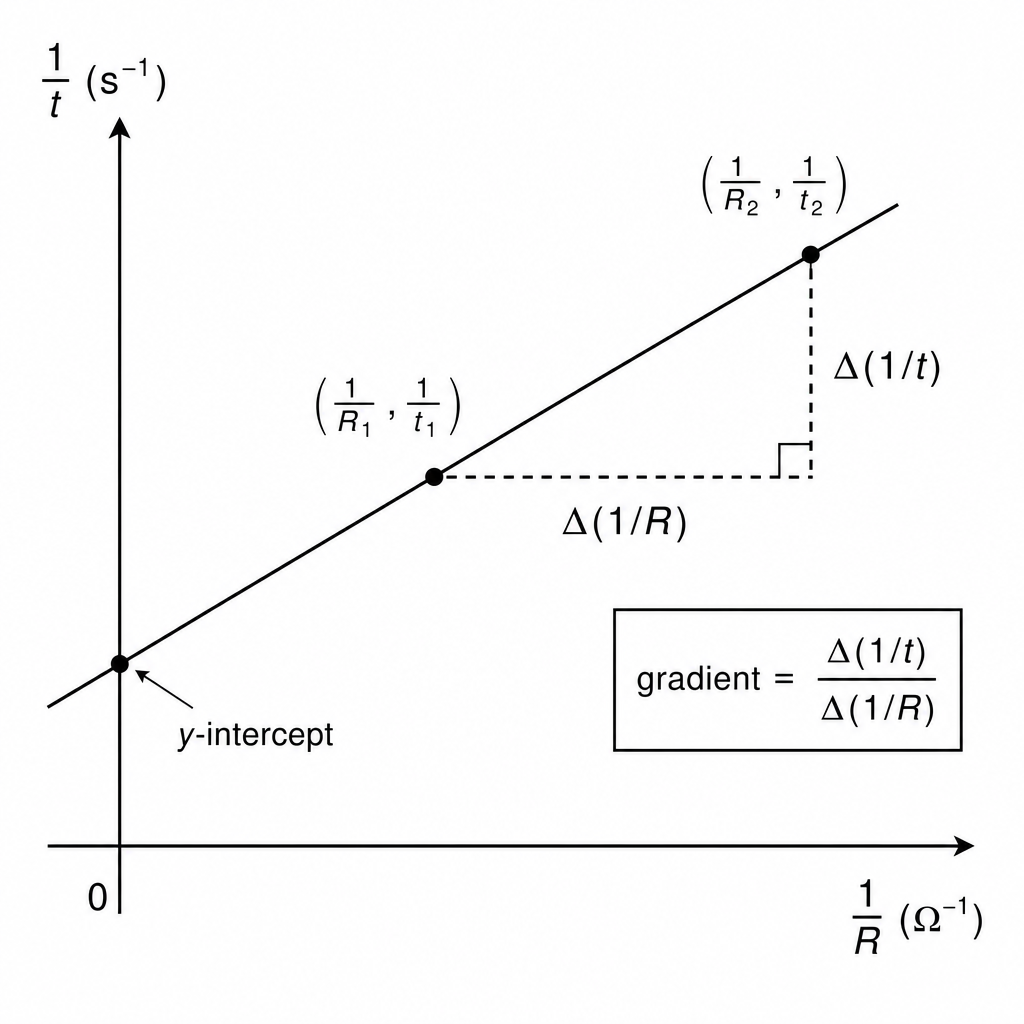
Choose two points on the best-fit line that are far apart to make a large triangle (reduces percentage reading error).
Read their coordinates carefully.
Compute $\Delta y$ and $\Delta x$ and divide to get the gradient.
Find the y-intercept by extending the best-fit line to $x=0$ and reading off $y$ .

gradient-triangle

Step-by-Step Reasoning

Pick two convenient points on the line (often where it crosses grid intersections). Do not necessarily use your plotted crosses.
Read $x_1, y_1$ and $x_2, y_2$ from the axes. Keep track of units: $x$ in $\Omega^{-1}$ and $y$ in $\text{s}^{-1}$ .
Calculate changes: $\Delta y = y_1 - y_2,\quad \Delta x = x_1 - x_2.$
Gradient: $m = \frac{\Delta y}{\Delta x}.$
Intercept: extend line to the $y$ -axis (where $x=0$ ) and read $c$ .

If your line is correct, different sensible point pairs on the line should give very similar gradients.

Key Takeaways

Always use the best-fit line and a large triangle to find the gradient.
Gradient and intercept must include correct units derived from the axes.

Common Mistakes

Using two adjacent plotted points (small triangle gives large uncertainty in gradient).
Calculating $\Delta x/\Delta y$ instead of $\Delta y/\Delta x$ .
Reading the intercept from the wrong axis or forgetting to extend the line to $x=0$ .

Things to Be Careful About

Use consistent significant figures: the gradient and intercept should reflect graph-reading precision.
Make sure you use $1/R$ values on the x-axis and $1/t$ values on the y-axis when reading coordinates.
Do not quote gradient units as $\text{s}^{-1}\ \Omega^{-1}$ ; simplify to $\Omega\ \text{s}^{-1}$ .

Techniques used

determine gradient from a large triangle on a best-fit linecalculate gradient using \Delta y / \Delta x with correct unitsread the y-intercept from the best-fit line

(e)

It is suggested that the quantities $t$ and $R$ are related by the equation

\frac{1}{t} = \frac{a}{R} + b

where $a$ and $b$ are constants.

Use your answers in (d)(iii) to determine the values of $a$ and $b$ .
Give appropriate units.

$a$ = ______
$b$ = ______

DifficultyMedium-Easy

Worked solution

Working

Given

\frac{1}{t} = \frac{a}{R} + b

Compare with $y = mx + c$ where $y = 1/t$ and $x = 1/R$ .

a = \text{gradient},\quad b = y\text{-intercept}

Units:

[b] = \text{s}^{-1},\quad [a] = \frac{\text{s}^{-1}}{\Omega^{-1}} = \Omega\ \text{s}^{-1}

Answer

$a = 8.0\ \Omega\ \text{s}^{-1}$

$b = 0.020\ \text{s}^{-1}$

Final answer

a = gradient (Ω s^-1), b = y-intercept (s^-1)

Detailed explanation

Background Concept

If a relationship can be written in the linear form

y = mx + c,

then on a graph of $y$ against $x$ :

the gradient is $m$ ,
the y-intercept is $c$ .

Here the suggested relationship is

\frac{1}{t} = \frac{a}{R} + b.

This already looks like a straight-line equation if we set $y = 1/t$ and $x = 1/R$ .

Understanding the Question

You have already found the gradient and y-intercept from your graph of $1/t$ (y-axis) against $1/R$ (x-axis). You must now use those values to identify the constants $a$ and $b$ , including appropriate units.

Approach

Rewrite the given equation in the form $y = mx + c$ by identifying $y$ and $x$ .
Match the constant multiplying $x$ to the gradient, and the constant term to the intercept.
Work out units from the quantities involved.

Step-by-Step Reasoning

Let

y = \frac{1}{t}, \quad x = \frac{1}{R}.

Then

\frac{1}{t} = \frac{a}{R} + b \;\Rightarrow\; y = a\left(\frac{1}{R}\right) + b = ax + b.

So the straight-line comparison gives:

gradient $m = a$
intercept $c = b$

Units:

$1/t$ has unit $\text{s}^{-1}$ .
$1/R$ has unit $\Omega^{-1}$ .
So

[a] = \frac{\text{s}^{-1}}{\Omega^{-1}} = \Omega\ \text{s}^{-1},

and

[b] = \text{s}^{-1}.

Key Takeaways

Once you have plotted the correct graph, constants in a linear equation come directly from the gradient and intercept.
Always deduce and state units for calculated constants.

Common Mistakes

Swapping $a$ and $b$ (writing $a$ as the intercept and $b$ as the gradient).
Giving $a$ the wrong units (e.g. $\text{s}^{-1}\ \Omega^{-1}$ instead of $\Omega\ \text{s}^{-1}$ ).

Things to Be Careful About

This matching only works because you plotted $1/t$ against $1/R$ in that order.
Ensure your gradient and intercept values are taken from the best-fit line (and therefore $a$ and $b$ are too).

Techniques used

compare an experimental straight-line graph with a given linear equationidentify constants from gradient and interceptdeduce correct units from a rearranged equation

The rest of this paper

1 more questions

Q2Manipulation, Measurement and Observation · Analysis, Conclusions and Evaluation · Presentation of Data and Observations20M

Loading the full paper…