Physics 9702/35 — October/November 2021

Cambridge AS Level · Advanced Practical Skills · worked solutions for every part, with the mark scheme

questions

marks

120

minutes

Topics Manipulation, Measurement and Observation · Presentation of Data and Observations · Analysis, Conclusions and Evaluation

Q1Manipulation, Measurement and ObservationPresentation of Data and ObservationsAnalysis, Conclusions and EvaluationFree sample

In this experiment, you will investigate the oscillations of a metre rule.

(a)

● Set up the apparatus as shown in Fig. 1.1, with the scales on the metre rules facing upwards.

Fig. 1.1

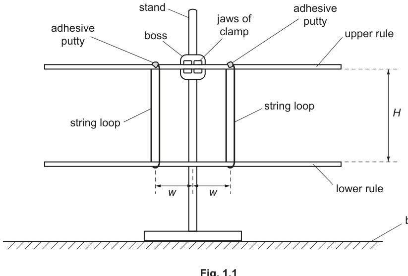
● Adjust the clamp so that the upper rule is parallel to the bench.
● Adjust the positions of the string loops so that each loop is approximately $40\text{ cm}$ from the nearest ends of the two rules.
● The vertical distance between the two rules is $H$ .

Measure and record $H$ .

$H$ = ______

DifficultyEasy

Worked solution

Answer

Measure the vertical distance between the two metre rules and record to the nearest mm.

Example: $H = 8.50\ \text{cm}$

Final answer

Example: H = 8.50 cm

Detailed explanation

Background Concept

In practical work, a mark is earned for making a sensible measurement and recording it with the correct unit and appropriate precision. The key ideas are:

measure the correct quantity (here a vertical separation),
use an appropriate instrument (metre rule / ruler, often helped by a set square),
avoid systematic errors (especially parallax),
record the reading to the instrument’s resolution (e.g. nearest $1\ \text{mm}$ ).

Understanding the Question

You have two metre rules, one above the other. The quantity $H$ is the vertical distance between the two rules (as labelled in the diagram). You must measure $H$ and write it down.

Approach

Identify two reference points: a point on the upper rule and the corresponding point directly beneath it on the lower rule.
Use a ruler/set square to measure the vertical separation.
Record the value with a unit and suitable precision (typically $0.1\ \text{cm}$ ).

Step-by-Step Reasoning

Ensure the upper rule is parallel to the bench (given instruction), so the separation is well-defined.
Place a ruler vertically (or use a set square to help keep it vertical) and measure the gap between the facing surfaces/edges of the two rules.
Read the scale with your eye level with the mark to avoid parallax.
Record as, for example, $H = 8.50\ \text{cm}$ (any sensible value depending on your set-up earns the mark if measured and recorded correctly).

Key Takeaways

Practical marks often reward good measurement technique and correct recording rather than one “correct” number.

Common Mistakes

Measuring along a slanted line rather than vertically.
Omitting the unit.
Recording too many decimal places (implying unrealistic precision) or too few (wasting available precision).

Things to Be Careful About

Ensure you are measuring the distance between the rules, not the height from the bench.
Keep the measuring device vertical and avoid parallax when reading the scale.

Techniques used

read a vertical separation using a ruler or set squarerecord a measurement to the appropriate precision with a unitavoid parallax when reading a scale

(b)

● For both rules, the distance between the $50\text{ cm}$ mark and each string loop is $w$ , as shown in Fig. 1.1.

Adjust the positions of the string loops until the distances $w$ are equal and approximately $10\text{ cm}$ .

● Measure and record $w$ .

$w$ = ______ $\text{cm}$

● Gently rotate the lower rule and release it. The lower rule will oscillate as shown in Fig. 1.2.

Fig. 1.2

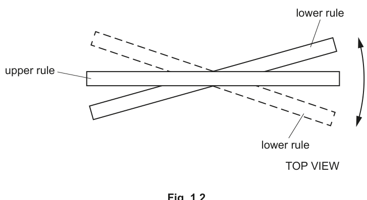
● Take measurements to determine the period $T$ of the oscillations.

$T$ = ______ $\text{s}$

DifficultyMedium-Easy

Worked solution

Answer

Set the two loops so that the distances from the $50\ \text{cm}$ mark are equal on both sides.

Measure $w$ (to nearest $1\ \text{mm}$ ).

Example: $w = 10.0\ \text{cm}$

To find $T$ , time $N$ oscillations (e.g. $N = 20$ ) and calculate $T = \dfrac{t}{N}$ .

Example: $t = 8.60\ \text{s}$ for $20$ oscillations, so

T = \frac{8.60}{20} = 0.430\ \text{s}

Final answer

Example: w = 10.0 cm, T = 0.430 s

Detailed explanation

Background Concept

The period $T$ is the time for one complete oscillation. A stopwatch reaction time is typically about $0.2\ \text{s}$ , which is large compared with a single short oscillation, so you improve reliability by timing many oscillations:

T = \frac{t}{N}

where $t$ is the total time for $N$ oscillations.

Understanding the Question

You must:

Adjust the string loops so that each loop is the same distance from the $50\ \text{cm}$ mark, and this distance is called $w$ .
Measure $w$ .
Make the lower rule oscillate and measure the period $T$ .

Approach

First make the geometry symmetrical (equal $w$ on both sides) so the motion is consistent.
Measure $w$ directly with the rule scale.
Measure $T$ by timing a large number of oscillations to reduce the effect of reaction time, then divide.

Step-by-Step Reasoning

Slide each string loop along the rule until the distance from the $50\ \text{cm}$ mark to each loop is the same (this is important for a balanced oscillation).
Read the distance $w$ from the scale, recording to the smallest sensible division (usually $0.1\ \text{cm}$ ).
Displace the lower rule slightly (small amplitude helps keep the motion regular) and release.
Start the stopwatch as a reference point passes the centre position, count $N$ full oscillations, and stop the watch at the same reference point.
Calculate $T = t/N$ .
Repeat timing at least once and use the mean $T$ if your times differ noticeably.

Key Takeaways

Time multiple oscillations and divide to obtain a better estimate of $T$ .
Symmetry (equal $w$ values) improves the consistency of the motion.

Common Mistakes

Timing just one oscillation (large percentage uncertainty).
Not defining a consistent start/stop point in the cycle.
Measuring $w$ from the end of the rule instead of from the $50\ \text{cm}$ mark.

Things to Be Careful About

Count complete oscillations (e.g. same orientation each cycle).
Keep the amplitude small and similar each time.
Record $w$ with unit ( $\text{cm}$ ) and $T$ with unit ( $\text{s}$ ).

Techniques used

adjust the apparatus to set an independent variable to a target valuemeasure a length with a ruler and record with unit and precisiondetermine a period by timing multiple oscillations and dividing

(c)

Vary $w$ in the range $5.0\text{ cm} \leq w \leq 20.0\text{ cm}$ and determine six sets of readings of $w$ and $T$ .

Record your results in a table. Include values of $\frac{1}{w}$ in your table.

DifficultyMedium

Worked solution

Answer

Take six values of $w$ in the range $5.0\ \text{cm} \le w \le 20.0\ \text{cm}$ and determine the corresponding $T$ .

Record in one table with headings and units, and include $1/w$ .

Example of a correctly presented table:

$w / \text{cm}$	$T / \text{s}$	$\left(1/w\right) / \text{cm}^{-1}$
$5.0$	$0.860$	$0.200$
$8.0$	$0.538$	$0.125$
$10.0$	$0.430$	$0.100$
$12.0$	$0.358$	$0.0833$
$16.0$	$0.269$	$0.0625$
$20.0$	$0.215$	$0.0500$

Final answer

Student-dependent (table of 6 readings of w and T with calculated 1/w).

Detailed explanation

Background Concept

Good experimental data presentation is assessed by:

using a single clear table,
putting the quantity and unit in the heading (not in the body of the table),
keeping consistent decimal places within a column,
calculating derived quantities correctly (here $1/w$ ) and recording them sensibly.

Understanding the Question

You must vary $w$ across the stated range and obtain six pairs of values $(w, T)$ . You must also calculate and include $1/w$ for each $w$ .

Here, $w$ is the independent variable (you change it) and $T$ is the dependent variable (you measure it). The extra column $1/w$ is needed later for graph plotting.

Approach

Choose six values of $w$ spread across $5.0\ \text{cm}$ to $20.0\ \text{cm}$ .
For each $w$ , measure the period $T$ using the multi-oscillation timing method.
Calculate $1/w$ for each reading and record everything in a well-formatted table.

Step-by-Step Reasoning

Select values such as $5.0$ , $8.0$ , $10.0$ , $12.0$ , $16.0$ , $20.0\ \text{cm}$ to cover the range.
For each $w$ , time $N$ oscillations (e.g. $N=20$ ) and compute $T=t/N$ .
Compute $1/w$ using:

\frac{1}{w}

For example, if $w = 12.0\ \text{cm}$ ,

\frac{1}{w} = \frac{1}{12.0} = 0.0833\ \text{cm}^{-1}

Record all values in a single table with headings such as $w/\text{cm}$ , $T/\text{s}$ , and $(1/w)/\text{cm}^{-1}$ .

Key Takeaways

A good table is part of the assessment: headings, units, and consistent precision matter.
Derived quantities (like $1/w$ ) must have correct units (here $\text{cm}^{-1}$ ).

Common Mistakes

Writing units in every cell instead of in the heading.
Using inconsistent decimal places in a column.
Calculating $1/w$ but not giving its unit.
Choosing values of $w$ that are clustered and do not cover the full range.

Things to Be Careful About

Ensure $w$ really lies between $5.0$ and $20.0\ \text{cm}$ .
Keep the timing method consistent for all readings.
Do not round $1/w$ so aggressively that plotting becomes inaccurate.

Techniques used

collect a suitable range of values for the independent variablerecord repeated measurements in a structured table with headings and unitscalculate a derived quantity from measured values with consistent significant figures

(d)

(i)

Plot a graph of $T$ on the $y$ -axis against $\frac{1}{w}$ on the $x$ -axis.

DifficultyMedium-Easy

Worked solution

Answer

Plot $T$ on the $y$ -axis and $1/w$ on the $x$ -axis.

Label axes with units: $T/\text{s}$ and $(1/w)/\text{cm}^{-1}$ .

Use a sensible scale occupying at least half the grid and plot all six points accurately.

Final answer

Graph of T (y) against 1/w (x), with correct labels and plotted points.

Detailed explanation

Background Concept

Graphs in Paper 3 are marked for:

correct choice of variables on each axis,
correct axis labels including units,
sensible scales (not cramped; not awkward values like 3 squares = 1 unit),
accurate plotting (small, neat points).

Understanding the Question

You are instructed to plot $T$ on the vertical axis and $1/w$ on the horizontal axis. The values come from your table in part (c).

Approach

Put $1/w$ on the $x$ -axis and $T$ on the $y$ -axis.
Decide scales so your data spans a good fraction of the graph paper.
Plot each point carefully from the table.

Step-by-Step Reasoning

Determine the range of $1/w$ . If $w$ is from $5.0$ to $20.0\ \text{cm}$ then $1/w$ will be from $0.200$ down to $0.0500\ \text{cm}^{-1}$ .
Determine the range of $T$ from your measurements.
Choose a scale such that these ranges take up at least half (preferably more) of each axis.
Label axes clearly as $T / \text{s}$ and $(1/w) / \text{cm}^{-1}$ .
Plot each point using a sharp pencil; a small cross or dot with a circle is typical.

Key Takeaways

Good scaling and correct labels are as important as the plotted points.

Common Mistakes

Swapping axes (plotting $T$ on $x$ and $1/w$ on $y$ ).
Missing units on axes.
Using a scale that wastes most of the grid.

Things to Be Careful About

Plot the reciprocal values ( $1/w$ ), not $w$ .
Keep the same rounding in your table and graph so points match your recorded values.

Techniques used

choose suitable axis scales that use most of the gridlabel axes with quantity and unitplot experimental points accurately

(ii)

Draw the straight line of best fit.

DifficultyEasy

Worked solution

Answer

Draw a single straight line of best fit with points distributed roughly equally above and below the line.

Final answer

Straight best-fit line drawn.

Detailed explanation

Background Concept

A best-fit line represents the overall trend of experimental data when random uncertainties cause scatter. For a relationship expected to be linear, you draw a single straight line that best represents the data.

Understanding the Question

You have already plotted $T$ against $1/w$ . Now you must draw the straight line that best fits the plotted points.

Approach

Use a ruler.
Aim for a balanced line: roughly equal numbers of points above and below, and similar distances.

Step-by-Step Reasoning

Place the ruler so that it follows the trend of the points.
Do not force the line through every point.
Draw one thin, clear straight line across as much of the graph as possible.

Key Takeaways

A best-fit line is about the overall trend, not joining dots.

Common Mistakes

Joining points with segments instead of one straight line.
Forcing the line through an outlier or through the origin without justification.

Things to Be Careful About

Extend the line well beyond the central cluster of points (within the plotted range) so that the gradient can be measured accurately.

Techniques used

draw a single straight line that balances scatter about itignore any small random scatter while fitting the trend

(iii)

Determine the gradient of this line.

gradient = ______

DifficultyMedium-Easy

Worked solution

Working

Choose two points on the best-fit line (far apart).

Example points: $(1/w, T) = (0.200\ \text{cm}^{-1},\ 0.860\ \text{s})$ and $(0.0500\ \text{cm}^{-1},\ 0.215\ \text{s})$ .

\text{gradient} = \frac{\Delta T}{\Delta(1/w)} = \frac{0.860 - 0.215}{0.200 - 0.0500}

\text{gradient} = \frac{0.645}{0.150} = 4.30\ \text{s cm}

Answer

gradient $= 4.30\ \text{s cm}$

Final answer

4.30 s cm

Detailed explanation

Background Concept

For a graph of $y$ against $x$ , the gradient $m$ is

m = \frac{\Delta y}{\Delta x}

The key practical skills are:

use the best-fit line, not individual plotted points,
take a large triangle (widely separated points) to reduce percentage reading error,
include units: here $y$ is $T$ in seconds and $x$ is $1/w$ in $\text{cm}^{-1}$ , so the gradient unit is $\text{s} / (\text{cm}^{-1}) = \text{s cm}$ .

Understanding the Question

You must find the gradient (slope) of your straight line on the graph of $T$ vs $1/w$ .

Approach

Pick two points on the drawn best-fit line that are far apart and easy to read.
Read their coordinates.
Compute $\Delta T$ and $\Delta(1/w)$ and divide.
Quote the gradient with a unit.

Step-by-Step Reasoning

diagram-1

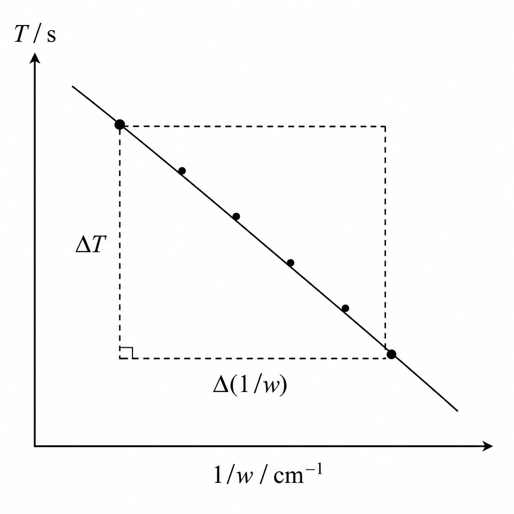
Suppose you read two well-separated points on the best-fit line:
- Point 1: $(x_1, y_1) = (0.200\ \text{cm}^{-1},\ 0.860\ \text{s})$
- Point 2: $(x_2, y_2) = (0.0500\ \text{cm}^{-1},\ 0.215\ \text{s})$
Differences:

\Delta T = y_1 - y_2 = 0.860 - 0.215 = 0.645\ \text{s}

\Delta(1/w) = x_1 - x_2 = 0.200 - 0.0500 = 0.150\ \text{cm}^{-1}

Gradient:

\text{gradient} = \frac{0.645}{0.150} = 4.30

Unit:

\text{unit} = \frac{\text{s}}{\text{cm}^{-1}} = \text{s cm}

So gradient $= 4.30\ \text{s cm}$ (your value depends on your best-fit line).

Key Takeaways

Always use $\Delta y/\Delta x$ from the best-fit line.
Use a large triangle and include units.

Common Mistakes

Using two nearby points (large uncertainty in gradient).
Using a plotted data point that is not on the best-fit line.
Calculating $\Delta x/\Delta y$ instead of $\Delta y/\Delta x$ .
Omitting the unit.

Things to Be Careful About

Read coordinates carefully from the axes (especially $1/w$ values).
Do not round the intermediate differences too aggressively; round at the end.
Ensure $\Delta(1/w)$ is not taken as negative (use consistent subtraction so the gradient stays positive).

Techniques used

select two well-separated points on a best-fit linecalculate gradient using $\Delta y / \Delta x$carry units through a gradient calculation

(e)

(i)

It is suggested that the quantities $T$ and $w$ are related by the equation

T = \frac{B}{w}

where $B$ is a constant.

Using your answer to (d)(iii), determine a value for $B$ .
Give an appropriate unit.

$B$ = ______

DifficultyMedium-Easy

Worked solution

Working

Given

T = \frac{B}{w}

and the graph is $T$ against $1/w$ , so

T = B\left(\frac{1}{w}\right)

Hence gradient $= B$ .

Using (d)(iii),

B = 4.30\ \text{s cm}

Answer

$B = 4.30\ \text{s cm}$

Final answer

4.30 s cm

Detailed explanation

Background Concept

A straight-line graph has the form

y = mx + c

where $m$ is the gradient and $c$ is the intercept. If an equation can be rearranged into this form using the variables you plotted, you can identify constants directly from the gradient/intercept.

Understanding the Question

You are told

T = \frac{B}{w}

and you have plotted $T$ (y-axis) against $1/w$ (x-axis). You must use your gradient from (d)(iii) to find $B$ and give its unit.

Approach

Rewrite the given equation so it contains the plotted variable $1/w$ explicitly, then match it to $y = mx + c$ .

Step-by-Step Reasoning

Starting from

T = \frac{B}{w}

multiply top and bottom idea: treat $1/w$ as a single quantity:

T = B\left(\frac{1}{w}\right)

So, comparing with $y = mx + c$ :

$y$ corresponds to $T$
$x$ corresponds to $1/w$
gradient $m$ corresponds to $B$
intercept $c$ should be close to $0$ (ideally).

Therefore your measured gradient equals $B$ .

Unit: if $T$ is in $\text{s}$ and $1/w$ is in $\text{cm}^{-1}$ , then

[B] = \frac{\text{s}}{\text{cm}^{-1}} = \text{s cm}

Key Takeaways

If you plot $T$ vs $1/w$ , the constant in $T = B(1/w)$ is the gradient.
Always deduce the unit from the graph axes.

Common Mistakes

Taking $B$ as the reciprocal of the gradient.
Giving unit $\text{s cm}^{-1}$ instead of $\text{s cm}$ .
Forgetting that the graph was against $1/w$ , not against $w$ .

Things to Be Careful About

Use the gradient from the best-fit line (not two raw points unless they are on the line).
Quote $B$ to a sensible number of significant figures consistent with your gradient.

Techniques used

compare an equation with y = mx + cidentify a constant from a graph gradientstate the correct unit for a derived constant

(ii)

It is suggested that $B$ is given by the equation

B^2 = \frac{3\pi^2 H^3}{g}

where $g$ is the acceleration of free fall.

Using your answers to (a) and (e)(i), determine a value for $g$ .

$g$ = ______ $\text{m s}^{-2}$

DifficultyMedium-Easy

Worked solution

Working

Convert to SI:

H = 8.50\ \text{cm} = 0.0850\ \text{m}

B = 4.30\ \text{s cm} = 0.0430\ \text{s m}

From

B^2 = \frac{3\pi^2 H^3}{g}

g = \frac{3\pi^2 H^3}{B^2}

g = \frac{3\pi^2(0.0850)^3}{(0.0430)^2} = 9.99\ \text{m s}^{-2}

Answer

$g = 10.0\ \text{m s}^{-2}$

Final answer

10.0 m s^-2

Detailed explanation

Background Concept

When you use a theoretical relationship to determine a constant (here $g$ ), you must:

rearrange the equation correctly,
substitute values with consistent units (usually SI),
handle powers carefully (here $H^3$ and $B^2$ ),
quote $g$ with unit $\text{m s}^{-2}$ .

Understanding the Question

You are given

B^2 = \frac{3\pi^2 H^3}{g}

You have measured $H$ in part (a) and found $B$ from the graph in (e)(i). You must calculate $g$ .

Approach

Rearrange to make $g$ the subject.
Convert $H$ and $B$ into SI units (metres, seconds).
Substitute and calculate.

Step-by-Step Reasoning

Rearrange:

B^2 = \frac{3\pi^2 H^3}{g} \quad \Rightarrow \quad g = \frac{3\pi^2 H^3}{B^2}

Convert units:

If $H$ was measured in cm, convert using $1\ \text{cm} = 10^{-2}\ \text{m}$ .
If $B$ was obtained in $\text{s cm}$ from the graph, convert to $\text{s m}$ by multiplying by $10^{-2}$ .

Substitute (example values):

H = 0.0850\ \text{m},\quad B = 0.0430\ \text{s m}

Compute:

$H^3 = (0.0850)^3\ \text{m}^3$
$B^2 = (0.0430)^2\ \text{s}^2\text{ m}^2$

Then

g = \frac{3\pi^2 H^3}{B^2}

The units give

\frac{\text{m}^3}{\text{s}^2\text{ m}^2} = \text{m s}^{-2}

which matches $g$ .

Key Takeaways

Always convert to SI before using formulas involving standard constants like $g$ .
Check units at the end to catch conversion errors.

Common Mistakes

Using $H$ in cm inside the formula (leading to $g$ wrong by factors of $10^6$ because of $H^3$ ).
Not converting $B$ from $\text{s cm}$ to $\text{s m}$ .
Rearrangement error (e.g. using $g = 3\pi^2 H^3 B^2$ ).

Things to Be Careful About

Powers amplify unit mistakes: converting cm to m and then cubing is crucial.
Use consistent significant figures based on your measured $H$ and your graph gradient.

Techniques used

rearrange an equation to make the required quantity the subjectconvert measurements to SI units before substitutionsubstitute measured values and calculate a derived constant

The rest of this paper

1 more questions

Q2Manipulation, Measurement and Observation · Analysis, Conclusions and Evaluation · Presentation of Data and Observations20M

Loading the full paper…