Physics 9702/33 — October/November 2021

Cambridge AS Level · Advanced Practical Skills · worked solutions for every part, with the mark scheme

questions

marks

120

minutes

Topics Manipulation, Measurement and Observation · Presentation of Data and Observations · Analysis, Conclusions and Evaluation

Q1Manipulation, Measurement and ObservationPresentation of Data and ObservationsAnalysis, Conclusions and EvaluationFree sample

In this experiment, you will investigate combinations of resistors in an electrical circuit.

(a)

Fig. 1.1. shows an electrical circuit.

Fig. 1.1

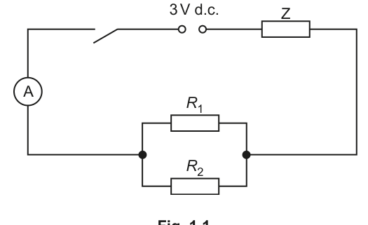
● Set up the circuit shown in Fig. 1.1 using $R_1 = 33\ \Omega$ and $R_2 = 82\ \Omega$ .

● Calculate $\frac{R_1R_2}{(R_1 + R_2)}$ .

$\frac{R_1R_2}{(R_1 + R_2)}$ = ______ $\Omega$

● Close the switch.

● Record the ammeter reading $I$ .

$I$ = ______

● Open the switch.

DifficultyMedium-Easy

Worked solution

Working

\frac{R_1R_2}{(R_1+R_2)}=\frac{(33)(82)}{(33+82)}

=\frac{2706}{115}=23.5\ \Omega

Ammeter reading recorded (example):

I = 0.069\ \text{A}

Answer

\frac{R_1R_2}{(R_1+R_2)} = 23.5\ \Omega

I = \text{(student reading)}

Final answer

23.5 Ω; I = (student reading)

Detailed explanation

Background Concept

Two resistors in parallel have the same potential difference across them, and the currents add. The equivalent resistance $R_{\text{p}}$ of two resistors $R_1$ and $R_2$ in parallel is defined by

\frac{1}{R_{\text{p}}}=\frac{1}{R_1}+\frac{1}{R_2}

Rearranging gives

R_{\text{p}}=\frac{R_1R_2}{(R_1+R_2)}

This is exactly the expression you are told to calculate.

Understanding the Question

You are given $R_1=33\ \Omega$ and $R_2=82\ \Omega$ . You must:

set up the circuit,
calculate the parallel combination value $\dfrac{R_1R_2}{(R_1+R_2)}$ ,
close the switch and record the current $I$ from the ammeter.

The current value depends on the rest of the circuit (including resistor $Z$ ), so it is “student-dependent”.

Approach

Compute $\dfrac{R_1R_2}{(R_1+R_2)}$ using straightforward substitution.
When measuring $I$ , ensure the ammeter is in series in the main branch, then record the reading to the ammeter’s resolution.

Step-by-Step Reasoning

Substitute the resistor values:

\frac{R_1R_2}{(R_1+R_2)}=\frac{(33)(82)}{33+82}

Calculate product and sum:

$R_1R_2 = 2706$
$R_1+R_2 = 115$
So

\frac{2706}{115}=23.530\ldots \approx 23.5\ \Omega

(rounded to 3 s.f.).

For the current, you close the switch and read the ammeter. A sensible recording would be to 2–3 s.f. depending on the meter scale (e.g. $0.069\ \text{A}$ if the display shows to $0.001\ \text{A}$ ).

Key Takeaways

Two resistors in parallel combine as $R_{\text{p}}=\dfrac{R_1R_2}{R_1+R_2}$ .
Practical marks often depend on correct set-up and correct recording (unit and appropriate precision).

Common Mistakes

Using the series formula $R_1+R_2$ instead of the parallel expression.
Arithmetic slip: adding $33+82$ incorrectly.
Recording $I$ without a unit or to inconsistent precision.

Things to Be Careful About

Keep units: the calculated quantity is in $\Omega$ .
Significant figures: resistors are given as integers, so 3 s.f. for the calculated value is reasonable.
Ensure the ammeter is in series (not across a component), otherwise it would short-circuit and give a wrong/unsafe reading.

Techniques used

calculate the equivalent resistance of two resistors in parallelsubstitute given resistor values and evaluate an expressiontake and record an ammeter reading to appropriate precision

(b)

Use six different pairs of resistors to provide six different values of $\frac{R_1R_2}{(R_1 + R_2)}$ .

For each arrangement, record $R_1$ , $R_2$ and $I$ in a table. Include values of $\frac{R_1R_2}{(R_1 + R_2)}$ and $\frac{1}{I}$ in your table.

10M

DifficultyMedium

Worked solution

Answer

Record six sets of readings in one table with headings (quantity and unit) and consistent precision.

Example of an acceptable table format (values shown are illustrative):

$R_1/\Omega$	$R_2/\Omega$	$\dfrac{R_1R_2}{(R_1+R_2)}/\Omega$	$I/\text{A}$	$\dfrac{1}{I}/\text{A}^{-1}$
$33$	$82$	$23.5$	$0.0690$	$14.5$
$47$	$100$	$32.0$	$0.0577$	$17.3$
$68$	$150$	$46.8$	$0.0449$	$22.3$
$100$	$220$	$68.8$	$0.0338$	$29.6$
$150$	$330$	$103$	$0.0244$	$41.0$
$220$	$470$	$150$	$0.0177$	$56.5$

(Any six suitable pairs with measured $I$ and correctly calculated columns score.)

Final answer

Table of six trials with R1, R2, R1R2/(R1+R2), I and 1/I (with units).

Detailed explanation

Background Concept

In this experiment, $R_1$ and $R_2$ form a parallel pair whose equivalent resistance is

R_{\text{p}}=\frac{R_1R_2}{(R_1+R_2)}

You then measure the circuit current $I$ for different values of $R_{\text{p}}$ . You are also asked to calculate $\dfrac{1}{I}$ , a derived quantity that is useful for later graph plotting.

Good experimental data presentation means:

one clear table,
headings with quantity and unit,
consistent significant figures/decimal places in each column.

Understanding the Question

You must choose six different resistor pairs $(R_1,R_2)$ such that the value of

\frac{R_1R_2}{(R_1+R_2)}

changes between trials. For each pair you must record:

$R_1$ and $R_2$ ,
the measured current $I$ ,
the calculated values of $\dfrac{R_1R_2}{(R_1+R_2)}$ and $\dfrac{1}{I}$ .

Approach

Pick resistor pairs that give a good spread of $R_{\text{p}}$ values (not all clustered).
For each pair:
- build the circuit,
- close the switch and allow reading to settle,
- record $I$ ,
- compute $R_{\text{p}}$ and $1/I$ .
Present everything in a single table with correct headings.
If time allows, repeat $I$ readings and average (improves quality of data).

Step-by-Step Reasoning

Choosing values: using both low and high resistor values generally gives a broader range of $R_{\text{p}}$ .
Calculating $R_{\text{p}}$ : do the product $R_1R_2$ and divide by the sum $R_1+R_2$ for each trial.
Measuring $I$ : keep the supply setting fixed, keep connections tight, and read the ammeter at eye level (if analogue) to reduce parallax.
Calculating $1/I$ : after measuring $I$ in amperes, compute the reciprocal; the unit becomes $\text{A}^{-1}$ .

Presentation details that typically earn marks:

Table heading such as $I/\text{A}$ (not just “I”).
Derived columns clearly labelled, e.g. $\dfrac{R_1R_2}{(R_1+R_2)}/\Omega$ and $\dfrac{1}{I}/\text{A}^{-1}$ .
Consistent precision down a column (e.g. all currents to 3 s.f. or all to the same number of decimal places, depending on meter resolution).

Key Takeaways

Collect enough points (six) and ensure they span a range.
Always include derived quantities in the table if you will need them for plotting.
Clear headings with units and consistent precision are essential in Paper 3.

Common Mistakes

Forgetting to include units in headings.
Mixing decimal places within a column (e.g. $0.06$ , $0.0577$ , $0.058$ ).
Choosing resistor pairs that give very similar $R_{\text{p}}$ values (graph then becomes less reliable).
Calculating $1/I$ using $I$ in mA but labelling the unit as $\text{A}^{-1}$ .

Things to Be Careful About

Use $I$ in amperes before taking the reciprocal.
Check that each calculated $R_{\text{p}}$ is less than both $R_1$ and $R_2$ (a quick check for a parallel combination).

Techniques used

select a suitable range of resistor pairs to span a range of equivalent resistancescompute derived quantities for each trialrecord results in a table with correct headings and unitsuse repeated readings to improve reliability

(c)

(i)

Plot a graph of $\frac{1}{I}$ on the $y$ -axis against $\frac{R_1R_2}{(R_1 + R_2)}$ on the $x$ -axis.

DifficultyMedium-Easy

Worked solution

Answer

Plot a graph with:

$y$ -axis: $\dfrac{1}{I}\ /\ \text{A}^{-1}$
$x$ -axis: $\dfrac{R_1R_2}{(R_1+R_2)}\ /\ \Omega$

Use a suitable scale (at least half the graph paper in each direction) and plot all six points accurately.

Final answer

Graph of 1/I (A^-1) against R1R2/(R1+R2) (Ω) plotted.

Detailed explanation

Background Concept

A graph is used to reveal the relationship between two quantities. To score well in Paper 3 graphing marks you must:

put the correct quantity on each axis,
label each axis with both the symbol/expression and the unit,
choose a scale that makes good use of the grid,
plot points accurately.

Understanding the Question

You are told exactly what to plot:

vertical axis is $\dfrac{1}{I}$ ,
horizontal axis is $\dfrac{R_1R_2}{(R_1+R_2)}$ .
You will use your six sets of data from part (b).

Approach

Decide the numerical ranges of $x$ and $y$ from your table.
Choose scales that cover the full range neatly (avoid awkward scales like 3 squares = 1 unit).
Label axes correctly and plot each point with a small, clear cross.

Step-by-Step Reasoning

From your results table, identify the minimum and maximum values of $\dfrac{R_1R_2}{(R_1+R_2)}$ and of $\dfrac{1}{I}$ .
Mark out axis scales so that the plotted points spread across the paper.
Axis labels should be written like:
- $\dfrac{1}{I}\ /\ \text{A}^{-1}$
- $\dfrac{R_1R_2}{(R_1+R_2)}\ /\ \Omega$
Plot each data pair $(x,y)$ .

Key Takeaways

Correct axes and correct units are essential.
Good scaling and accurate plotting improves the gradient/intercept accuracy later.

Common Mistakes

Swapping axes (plotting $\dfrac{1}{I}$ on $x$ ).
Missing units or writing units incorrectly.
Using a tiny portion of the grid so the best-fit line is poorly determined.

Things to Be Careful About

Ensure $I$ is in amperes before calculating $1/I$ .
Keep the same number of significant figures in $1/I$ as justified by the precision of $I$ .

Techniques used

choose appropriate axes for a specified graphlabel axes with quantity and unitselect a sensible scale that uses most of the gridplot experimental points accurately

(ii)

Draw the straight line of best fit.

DifficultyEasy

Worked solution

Answer

Draw a single straight line of best fit with points approximately balanced above and below the line (do not join point-to-point).

Final answer

Straight line of best fit drawn.

Detailed explanation

Background Concept

A best-fit line represents the overall trend of the data and is used to find the gradient and intercept. For experimental data, points rarely lie perfectly on a line due to random uncertainties.

Understanding the Question

After plotting the six points, you must draw the straight line that best represents the relationship between $\dfrac{1}{I}$ and $\dfrac{R_1R_2}{(R_1+R_2)}$ .

Approach

Use a ruler.
Place the line so that the vertical distances (residuals) of points from the line are reasonably balanced: similar scatter above and below.

Step-by-Step Reasoning

Do not connect dots sequentially; that creates a broken line and is not a best-fit line.
Do not automatically force the line through the origin unless your plotted points clearly support that (and the relationship predicts it).
Extend the line across most of the graph so you can later take a large gradient triangle.

Key Takeaways

Best-fit means “balanced scatter”, not “through the most points”.

Common Mistakes

Drawing a line that passes through every point by zig-zagging.
Forcing the line through the origin when there is a clear non-zero intercept.

Things to Be Careful About

Use a sharp pencil and a ruler; a thick line makes gradient reading less accurate.

Techniques used

judge scatter and draw a balanced best-fit straight lineavoid point-to-point joining and avoid forcing the line through the origin

(iii)

Determine the gradient and $y$ -intercept of this line.

gradient = ______

$y$ -intercept = ______

DifficultyMedium

Worked solution

Working

Using two well-separated points on the best-fit line (example):

(x_1,y_1)=(23.5\ \Omega,\ 14.5\ \text{A}^{-1}),\quad (x_2,y_2)=(150\ \Omega,\ 56.5\ \text{A}^{-1})

\text{gradient } m=\frac{\Delta y}{\Delta x}=\frac{56.5-14.5}{150-23.5}=\frac{42.0}{126.5}=0.332\ \text{A}^{-1}\ \Omega^{-1}

$y$ -intercept (example):

c \approx 6.67\ \text{A}^{-1}

Answer

\text{gradient} \approx 0.33\ \text{A}^{-1}\ \Omega^{-1}

y\text{-intercept} \approx 6.7\ \text{A}^{-1}

Final answer

gradient ≈ 0.33 A^-1 Ω^-1; y-intercept ≈ 6.7 A^-1

Detailed explanation

Background Concept

For a straight-line graph, the equation is

y = mx + c

where:

$m$ is the gradient (slope),
$c$ is the $y$ -intercept (value of $y$ when $x=0$ ).

On a plot of $\dfrac{1}{I}$ (vertical) against $\dfrac{R_1R_2}{(R_1+R_2)}$ (horizontal), the gradient has units

\frac{\text{A}^{-1}}{\Omega}=\text{A}^{-1}\ \Omega^{-1}

and the intercept has units $\text{A}^{-1}$ .

Understanding the Question

You must use your best-fit line (not individual points) to find:

the gradient,
the $y$ -intercept.

Approach

Take two points far apart on the drawn best-fit line to reduce percentage reading error.
Compute

\text{gradient} = \frac{\Delta y}{\Delta x}

Find the $y$ -intercept by reading where the line crosses the $y$ -axis (at $x=0$ ).

Step-by-Step Reasoning

Choose two points on the line that are convenient to read accurately (often at grid intersections). They do not have to be original data points.
Work out the changes:
- $\Delta y = y_2-y_1$ in $\text{A}^{-1}$
- $\Delta x = x_2-x_1$ in $\Omega$
Divide to obtain the gradient in $\text{A}^{-1}\ \Omega^{-1}$ .
For the intercept, extend the best-fit line to meet the $y$ -axis and read off $y$ at $x=0$ .

Key Takeaways

Always use the best-fit line, and use a large triangle.
Quote gradient and intercept with appropriate units.

Common Mistakes

Using $\dfrac{\Delta x}{\Delta y}$ instead of $\dfrac{\Delta y}{\Delta x}$ .
Using two nearby points (large uncertainty in gradient).
Forgetting units, or giving gradient units as just $\Omega$ or just $\text{A}^{-1}$ .

Things to Be Careful About

Read values from the line, not from the nearest plotted cross if it is not exactly on the line.
Ensure your axis scales are correctly interpreted (check each major square value before reading coordinates).

Techniques used

determine the gradient using a large triangle on the best-fit lineread the y-intercept from the graphcalculate the ratio \Delta y/\Delta x with correct units

(d)

(i)

It is suggested that the quantities $I$ and $\frac{R_1R_2}{(R_1 + R_2)}$ are related by the equation

\frac{1}{I} = P \left[ \frac{R_1R_2}{(R_1 + R_2)} \right] + Q

where $P$ and $Q$ are constants.

Using your answers to (c)(iii), determine the values of $P$ and $Q$ . Give appropriate units.

$P$ = ______

$Q$ = ______

DifficultyMedium-Easy

Worked solution

Working

Given

\frac{1}{I}=P\left[\frac{R_1R_2}{(R_1+R_2)}\right]+Q

Comparing with $y=mx+c$ :

P=\text{gradient},\quad Q=\text{y-intercept}

Using (c)(iii) (example):

P \approx 0.33\ \text{A}^{-1}\ \Omega^{-1}

Q \approx 6.7\ \text{A}^{-1}

Answer

P = \text{gradient}\ (\text{A}^{-1}\ \Omega^{-1})

Q = y\text{-intercept}\ (\text{A}^{-1})

Final answer

P = gradient (A^-1 Ω^-1); Q = y-intercept (A^-1)

Detailed explanation

Background Concept

If you plot $y$ against $x$ and obtain a straight line, you can compare the equation you are testing with

y = mx + c

Here,

y=\frac{1}{I},\quad x=\frac{R_1R_2}{(R_1+R_2)}

so the suggested relationship

\frac{1}{I} = P\left[\frac{R_1R_2}{(R_1+R_2)}\right]+Q

means:

$P$ is the gradient,
$Q$ is the $y$ -intercept.

Units:

$y$ has units $\text{A}^{-1}$ ,
$x$ has units $\Omega$ ,
so

[P] = \frac{\text{A}^{-1}}{\Omega}=\text{A}^{-1}\ \Omega^{-1},\quad [Q]=\text{A}^{-1}.

Understanding the Question

You are told to use your values from (c)(iii). That means you simply transfer your measured gradient to $P$ and your intercept to $Q$ , including units.

Approach

Identify $y$ , $x$ , gradient, intercept.
Set $P = \text{gradient}$ and $Q = \text{intercept}$ .
Attach correct units based on what was plotted.

Step-by-Step Reasoning

From your graph result:
- gradient $m$ becomes $P$ .
- intercept $c$ becomes $Q$ .
Write the values with units.

Key Takeaways

Matching to $y=mx+c$ is a powerful way to extract constants from experimental graphs.
Units come from the axes.

Common Mistakes

Swapping $P$ and $Q$ .
Writing unit for $P$ as $\Omega\ \text{A}^{-1}$ (it should be per ohm: $\Omega^{-1}\ \text{A}^{-1}$ ).

Things to Be Careful About

Use your best-fit line values, not values from two random plotted points.
Keep consistent significant figures (typically 2–3 s.f. for graphical quantities).

Techniques used

match a straight-line graph to y = mx + cidentify constants from the gradient and interceptassign units to constants from the plotted axes

(ii)

The constants $P$ and $Q$ are related to the electromotive force (e.m.f.) $E$ of the power supply and the resistance $Z$ of resistor $Z$ by

P = \frac{1}{E} \text{ and } Q = \frac{Z}{E}

Determine the values of $E$ and $Z$ . Give appropriate units.

$E$ = ______

$Z$ = ______

DifficultyMedium-Easy

Worked solution

Working

Given

P=\frac{1}{E},\quad Q=\frac{Z}{E}

E=\frac{1}{P}

Using $P\approx 0.332\ \text{A}^{-1}\ \Omega^{-1}$ (example):

E\approx \frac{1}{0.332}=3.01\ \text{V}

And

Z=EQ

Using $Q\approx 6.67\ \text{A}^{-1}$ (example):

Z\approx (3.01)(6.67)=20.1\ \Omega

Answer

E \approx 3.0\ \text{V}

Z \approx 20\ \Omega

Final answer

E ≈ 3.0 V; Z ≈ 20 Ω

Detailed explanation

Background Concept

From the graph,

\frac{1}{I} = P\left[\frac{R_1R_2}{(R_1+R_2)}\right] + Q

You are told that these constants link to the circuit parameters by

P=\frac{1}{E},\quad Q=\frac{Z}{E}

So:

$E$ is found by inverting $P$ .
Once $E$ is known, $Z$ is found from $Z = EQ$ .

Unit check:

Since $P=1/E$ , the unit of $P$ must be $\text{V}^{-1}$ . From the graph we found $P$ has unit $\text{A}^{-1}\ \Omega^{-1}$ , and indeed $\Omega\,\text{A} = \text{V}$ , so $\text{A}^{-1}\ \Omega^{-1} = \text{V}^{-1}$ .

Understanding the Question

You must calculate numerical values of:

$E$ (the e.m.f. of the supply, in volts),
$Z$ (the resistance of resistor $Z$ , in ohms),
using your experimentally determined $P$ and $Q$ .

Approach

Compute $E=1/P$ .
Compute $Z=EQ$ .
Quote answers with appropriate significant figures and correct units.

Step-by-Step Reasoning

Start with $P=1/E$ .
Rearranging gives $E=\frac{1}{P}$
Then from $Q=Z/E$ , rearrange: $Z=EQ$
Substitute your values of $P$ and $Q$ from the graph.

If your graph was good, $E$ should be close to the stated supply value (often around $3\ \text{V}$ in this set-up).

Key Takeaways

Graph constants can be converted into physical circuit parameters by algebraic rearrangement.
Checking units (e.g. $\Omega\,\text{A}=\text{V}$ ) helps confirm you have not inverted the wrong quantity.

Common Mistakes

Using $E=P$ instead of $E=1/P$ .
Using $Z=Q/E$ instead of $Z=EQ$ .
Forgetting units, especially for $E$ (must be V).

Things to Be Careful About

Use consistent significant figures: graphical gradients/intercepts are usually only 2–3 s.f.
If your $P$ has large uncertainty, $E=1/P$ will inherit that uncertainty (so avoid over-precise final digits).

Techniques used

rearrange constants to determine physical quantitiesinvert a measured gradient to obtain a parameteruse dimensional consistency to assign correct units

The rest of this paper

1 more questions

Q2Manipulation, Measurement and Observation · Presentation of Data and Observations · Analysis, Conclusions and Evaluation20M

Loading the full paper…