In this experiment, you will investigate the equilibrium of a plastic cup. (a) You have been provided with a cup attached to a string loop. A mass is attached to the cup as shown in Fig. 1.1. ● Set up the apparatus as shown in Fig. 1.2. ● The horizontal distance between the edges of the cup is $p$, as shown in Fig. 1.2. Measure and record $p$. $p$ = \_\_\_\_\_\_ (b) ● Pour approximately $12\ \text{cm}^3$ of water into the measuring cylinder. ● The mass of $1\ \text{cm}^3$ of…

Physics 9702/31 — October/November 2020

Cambridge AS Level · Advanced Practical Skills · worked solutions for every part, with the mark scheme

questions

marks

120

minutes

Topics Manipulation, Measurement and Observation · Presentation of Data and Observations · Analysis, Conclusions and Evaluation

Q1Manipulation, Measurement and ObservationPresentation of Data and ObservationsAnalysis, Conclusions and EvaluationFree sample

In this experiment, you will investigate the equilibrium of a plastic cup.

(a)

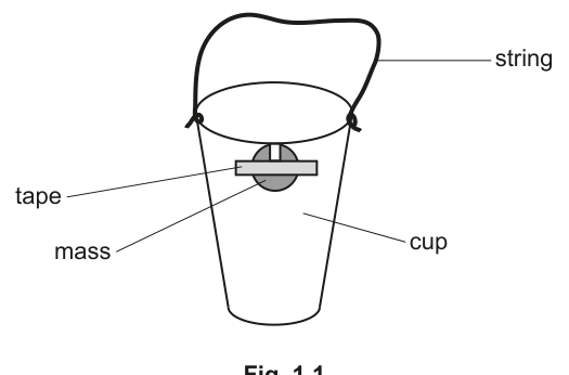
You have been provided with a cup attached to a string loop. A mass is attached to the cup as shown in Fig. 1.1.

Fig. 1.1

● Set up the apparatus as shown in Fig. 1.2.

Fig. 1.2

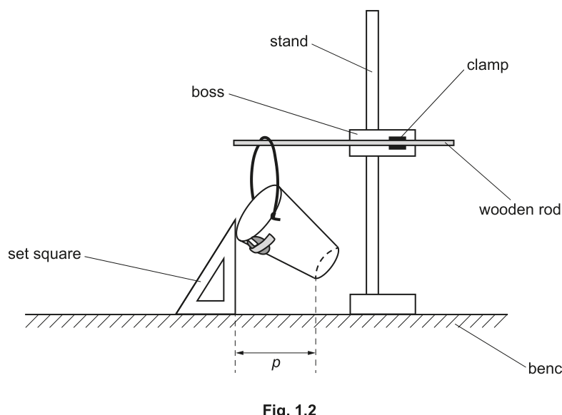
● The horizontal distance between the edges of the cup is $p$ , as shown in Fig. 1.2.

Measure and record $p$ .

$p$ = ______

DifficultyEasy

Worked solution

Answer

Measure the horizontal distance $p$ between the two cup edges using a ruler (read at eye level).

A typical reading:
$p = 6.0\ \text{cm}$ (to the nearest $0.1\ \text{cm}$ ).

Final answer

p = 6.0 cm

Detailed explanation

Background Concept

In a practical, a “measurement mark” is earned by:

using the instrument appropriately (e.g. a ruler for length),
measuring the correct quantity (here, a horizontal distance), and
recording the value with sensible precision that matches the instrument scale.

A standard mm ruler typically allows readings to the nearest $1\ \text{mm}$ , i.e. $0.1\ \text{cm}$ .

Understanding the Question

You are shown the cup hanging at an angle. The distance $p$ is defined as the horizontal distance between the two vertical edges of the cup (as drawn in Fig. 1.2). You must measure and record $p$ .

Approach

Set up the apparatus as shown.
Use a set square to define/transfer a horizontal line (so you do not accidentally measure along a sloping line).
Use a ruler to measure between the two relevant edges.
Record $p$ with unit and appropriate decimal places.

Step-by-Step Reasoning

diagram-1a

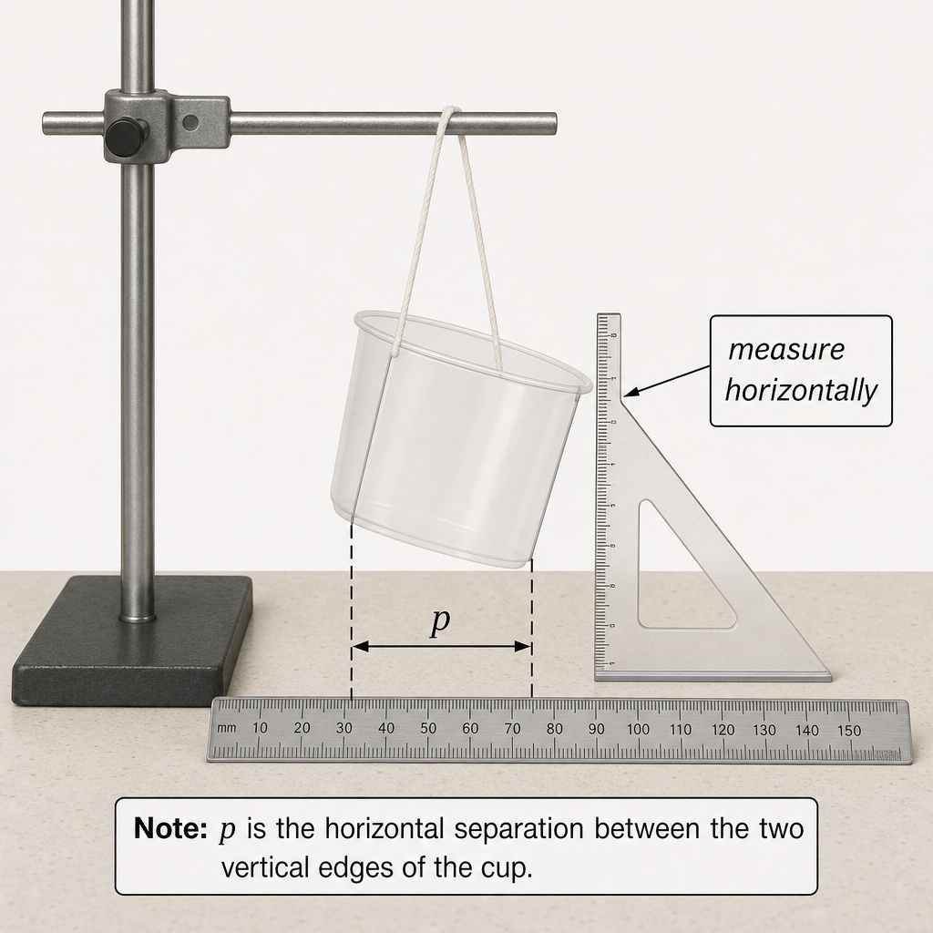
Identify the two cup edges between which $p$ is defined.
Place the set square so one edge is horizontal on the bench, and the vertical edge is next to one cup edge.
Use the set square to ensure you are measuring the horizontal separation.
Measure the distance between the two vertical edges using a ruler.
Read the scale at eye level to reduce parallax.
Record the value, e.g. $p = 6.0\ \text{cm}$ .

Key Takeaways

Measure the quantity that is defined (horizontal distance, not slanted distance).
Use a set square to help ensure true horizontal/vertical alignment.
Record with appropriate precision and unit.

Common Mistakes

Measuring along the sloping rim instead of horizontally.
Not including a unit.
Giving too many/few decimal places (e.g. $6.000\ \text{cm}$ or $6\ \text{cm}$ with a mm ruler).
Parallax error from reading the ruler at an angle.

Things to Be Careful About

Ensure you measure between the correct two edges (as indicated in the diagram).
Keep the ruler aligned horizontally; small misalignment changes $p$ noticeably.
If the cup is moving, wait for it to come to rest before reading.

Techniques used

align a ruler/set square to measure a horizontal distancetake a reading at eye level to reduce parallaxrecord a length to an appropriate precision

(b)

● Pour approximately $12\ \text{cm}^3$ of water into the measuring cylinder.

● The mass of $1\ \text{cm}^3$ of water is $1\ \text{g}$ .

Determine the mass of water in the measuring cylinder.

$\text{mass}$ = ______ $\text{g}$

● Gently pour this water from the measuring cylinder into the cup.

● Record the total mass $m$ of water in the cup.

$m$ = ______ $\text{g}$

● Measure and record $p$ .

$p$ = ______

DifficultyEasy

Worked solution

Working

Volume of water $\approx 12\ \text{cm}^3$ and $1\ \text{cm}^3$ has mass $1\ \text{g}$ , so

\text{mass} = 12\ \text{g}

After pouring into the cup, total mass of water in cup:

m = 12\ \text{g}

Typical measured value:

p = 6.1\ \text{cm}

Answer

$\text{mass} = 12\ \text{g}$

$m = 12\ \text{g}$

$p = 6.1\ \text{cm}$

Final answer

mass = 12 g; m = 12 g; p = 6.1 cm

Detailed explanation

Background Concept

The question uses the fact that water has density about $1\ \text{g cm}^{-3}$ .
That means:

each $1\ \text{cm}^3$ of water has mass $1\ \text{g}$ ,
so numerically the mass in grams equals the volume in $\text{cm}^3$ .

Understanding the Question

You first measure about $12\ \text{cm}^3$ of water in a measuring cylinder. You must:

determine the mass of that water,
pour it into the cup and record the total mass $m$ now in the cup (which should equal the mass you just calculated, assuming no spills),
measure the new value of $p$ .

Approach

Convert volume to mass using $1\ \text{cm}^3 \to 1\ \text{g}$ .
Pour carefully to keep $m$ equal to the calculated mass.
Re-measure $p$ in the same way as part (a).

Step-by-Step Reasoning

Measuring cylinder reading: $V \approx 12\ \text{cm}^3$ .
Using the given relationship for water:

\text{mass of water} = V \times 1\ \text{g cm}^{-3} = 12\ \text{g}

Pour into the cup carefully so the mass in the cup is still $m = 12\ \text{g}$ .
Measure $p$ again (cup angle changes when water is added), keeping the measurement horizontal and reading at eye level.

Key Takeaways

Use given density information to convert between volume and mass.
Re-measure the dependent variable ( $p$ ) each time you change $m$ .

Common Mistakes

Writing $12\ \text{g}$ for the cylinder but then recording a different $m$ in the cup without justification (usually due to spilling/incorrect reading).
Forgetting units.
Not re-measuring $p$ after adding water.

Things to Be Careful About

The instruction says “approximately $12\ \text{cm}^3$ ”: record what you actually measure if your cylinder reading is, for example, $11.5\ \text{cm}^3$ .
Avoid loss of water during transfer (pour slowly, use a funnel if available).
Keep the same method for measuring $p$ each time for consistency.

Techniques used

convert volume to mass using density informationtransfer liquid carefully to avoid lossmeasure and record a length after changing an experimental condition

(c)

Using the measuring cylinder, add water to the cup to increase $m$ . Measure and record $p$ . Repeat until you have six sets of values of $m$ and $p$ .

Record your results in a table. Include values of $\sqrt{m}$ and $\sqrt{p}$ in your table.

10M

DifficultyMedium

Worked solution

Answer

Record six sets of $m$ and $p$ and calculate $\sqrt{m}$ and $\sqrt{p}$ .

A suitable table format (example values shown):

$m$ / $\text{g}$	$p$ / $\text{cm}$	$\sqrt{m}$ / $\text{g}^{1/2}$	$\sqrt{p}$ / $\text{cm}^{1/2}$
12	6.12	3.46	2.47
22	6.42	4.69	2.53
32	6.67	5.66	2.58
42	6.89	6.48	2.62
52	7.08	7.21	2.66
62	7.26	7.87	2.69

Final answer

Single results table with columns m / g, p / cm, sqrt(m) / g^{1/2}, sqrt(p) / cm^{1/2} (six sets of readings).

Detailed explanation

Background Concept

Good experimental data handling is about two things:

Quality and range of raw data: you need enough readings (here six) and they should span a sensible range of the independent variable so that a trend/line can be seen.
Correct presentation: one clear table, clear headings with units, and consistent precision. If you calculate extra columns (like square roots), those must be calculated correctly and recorded to a sensible number of significant figures (often 3 s.f. for derived values).

Understanding the Question

You will increase the total mass of water $m$ in the cup by adding more water. For each value of $m$ , you measure $p$ .
You must obtain six pairs $(m, p)$ and present them in a single table. You must also include the calculated columns $\sqrt{m}$ and $\sqrt{p}$ .

Approach

Treat $m$ as the independent variable (you control it by adding water).
Measure $p$ as the dependent variable.
Take six values of $m$ spread out (not all very close together).
For each row, compute:

\sqrt{m} \quad \text{and} \quad \sqrt{p}

Present in a single table with headings “quantity / unit”.

Step-by-Step Reasoning

Start with the initial water amount from part (b), then add water in steps (e.g. $\sim 10\ \text{cm}^3$ at a time) until you have six readings.
Each time:
- Determine $m$ from the measuring cylinder addition(s) (using $1\ \text{cm}^3 \leftrightarrow 1\ \text{g}$ ).
- Wait for the cup to come to rest.
- Measure $p$ horizontally using the same method each time.
Create a table with columns:
- $m / \text{g}$ ,
- $p / \text{cm}$ ,
- $\sqrt{m} / \text{g}^{1/2}$ ,
- $\sqrt{p} / \text{cm}^{1/2}$ .
Use consistent decimal places for $p$ (e.g. to $0.1\ \text{cm}$ or $0.01\ \text{cm}$ depending on your ruler and how precisely you can judge the edges).
Use consistent significant figures (commonly 3 s.f.) for the square roots.

Key Takeaways

Six readings and a decent range make the later graph meaningful.
Headings must include both quantity and unit.
Derived columns must be calculated correctly and presented sensibly.

Common Mistakes

Splitting results into multiple small tables instead of one.
Missing units in headings (e.g. writing just “ $m$ ” rather than “ $m / \text{g}$ ”).
Inconsistent precision within a column (e.g. $6.1$ , $6.23$ , $7$ in the same column).
Incorrect square-root calculations or rounding too aggressively.

Things to Be Careful About

If you repeat readings of $p$ at the same $m$ , you can average them to improve reliability (and note this clearly).
Avoid very small changes in $m$ that produce changes in $p$ smaller than your measurement resolution.
Check calculator mode and rounding: record enough s.f. so the graph is not spoiled by rounding.

Techniques used

choose a suitable range and number of readings for the independent variablerecord results in a single table with headings and unitscalculate derived quantities using a calculatoruse consistent significant figures within each column

(d)

(i)

Plot a graph of $\sqrt{p}$ on the $y$ -axis against $\sqrt{m}$ on the $x$ -axis.

DifficultyMedium

Worked solution

Answer

Plot a graph of $\sqrt{p}$ (y-axis) against $\sqrt{m}$ (x-axis) with:

axes labelled $\sqrt{m} / \text{g}^{1/2}$ and $\sqrt{p} / \text{cm}^{1/2}$ ,
a suitable linear scale using most of the grid,
all six points plotted accurately.

Final answer

Graph of sqrt(p) (y) against sqrt(m) (x) with correct labels/units, suitable scale, and six plotted points.

Detailed explanation

Background Concept

When plotting experimental graphs, you gain marks for:

Correct choice of axes (right variables on right axes),
Correct labelling (quantity and unit),
Good scale (simple steps like 1, 2, 5; using at least half the grid),
Accurate plotting (small, neat points/crosses).

Using transformed variables (here square roots) is a common way to linearise a relationship so the data should lie close to a straight line.

Understanding the Question

You have a table including $\sqrt{m}$ and $\sqrt{p}$ . You must plot $\sqrt{p}$ on the vertical axis and $\sqrt{m}$ on the horizontal axis.

Approach

Put $\sqrt{m}$ on the x-axis (independent variable) and $\sqrt{p}$ on the y-axis (dependent variable).
Choose axis limits that just include your smallest and largest values.
Use a simple scale so you can plot precisely.

Step-by-Step Reasoning

diagram-1di

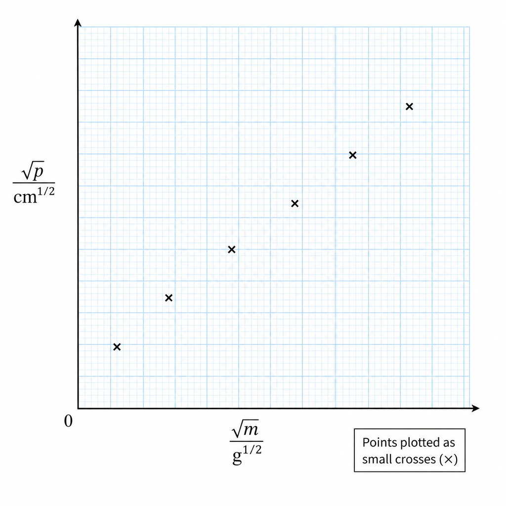
From your table, identify the min/max of $\sqrt{m}$ and $\sqrt{p}$ .
Draw axes and label them:
- x-axis: $\sqrt{m} / \text{g}^{1/2}$
- y-axis: $\sqrt{p} / \text{cm}^{1/2}$
Choose scales so that:
- the plotted points span a large fraction of the graph area,
- each large square corresponds to a convenient increment.
Plot each point as a small cross; if a point is wrong, clearly cross it out and replot.

Key Takeaways

Correct axes and labels are essential: without them, the graph cannot be interpreted.
A good scale makes gradient/intercept readings much more accurate.

Common Mistakes

Swapping axes (plotting $\sqrt{m}$ on y-axis).
Missing units or writing units incorrectly in the label.
Using awkward scales (e.g. 3 squares = 1 unit), wasting graph space.
Plotting $m$ and $p$ instead of $\sqrt{m}$ and $\sqrt{p}$ .

Things to Be Careful About

Check you are using the square-root columns from your table.
Do not force the graph through the origin unless the data and question justify it.
Make sure the plotted points are not dots so large that they hide the true position.

Techniques used

select appropriate axis variables and labelschoose a scale that uses at least half the graph paperplot points accurately from a data tablelabel axes with quantity and unit

(ii)

Draw the straight line of best fit.

DifficultyMedium-Easy

Worked solution

Answer

Draw a single straight line of best fit (not point-to-point), with roughly equal scatter of points about the line.

Final answer

Straight line of best fit drawn.

Detailed explanation

Background Concept

A best-fit line represents the overall trend in data that should be linear. For Cambridge practical marking, the line should:

be straight (if a straight-line relationship is expected),
be drawn with a ruler,
balance the scatter (similar number of points above and below),
extend across the region of the plotted points.

Understanding the Question

After plotting $\sqrt{p}$ against $\sqrt{m}$ , you must draw the best straight line through the data.

Approach

Use a ruler and aim for a line that represents the trend, not one that passes through every point.

Step-by-Step Reasoning

Place a ruler so the line passes through the middle of the “cloud” of points.
Adjust to make the vertical deviations of points above and below roughly balanced.
Draw the line across the full spread of x-values (not just a short segment).

Key Takeaways

A best-fit line is about overall trend, not connecting data points.

Common Mistakes

Joining points one by one.
Drawing a line that deliberately passes through an outlier.
Drawing a line that is too short (making gradient reading inaccurate).

Things to Be Careful About

If one point is clearly anomalous, the best-fit line should follow the majority trend (unless you have reason to believe all points are equally reliable).
Use a sharp pencil so the line thickness doesn’t dominate reading accuracy.

Techniques used

draw a single straight line that balances scatteravoid joining point-to-pointextend the line across the full data range

(iii)

Determine the gradient and $y$ -intercept of this line.

$\text{gradient}$ = ______
$\text{y-intercept}$ = ______

DifficultyMedium

Worked solution

Working

Using two well-separated points on the best-fit line, e.g.
$(\sqrt{m},\sqrt{p}) = (3.46,\ 2.47)$ and $(7.87,\ 2.69)$ :

\text{gradient} = \frac{\Delta \sqrt{p}}{\Delta \sqrt{m}} = \frac{2.69 - 2.47}{7.87 - 3.46} = 0.050

\text{y-intercept} = 2.30

Answer

$\text{gradient} = 0.050$

$\text{y-intercept} = 2.30$

Final answer

gradient = 0.050; y-intercept = 2.30

Detailed explanation

Background Concept

For a straight-line graph $y = mx + c$ :

the gradient is $m = \Delta y / \Delta x$ using two points on the line (not necessarily data points),
the y-intercept is $c$ , where the line crosses the y-axis (i.e. at $x=0$ ).

Using a large triangle (widely separated points) reduces percentage uncertainty in the gradient.

Understanding the Question

You have drawn a best-fit line on a plot of $\sqrt{p}$ (y) against $\sqrt{m}$ (x). You must find:

the gradient of this line,
the y-intercept of this line.

Approach

Pick two points on the drawn best-fit line that are far apart and easy to read.
Read their coordinates carefully.
Compute gradient as $\Delta y / \Delta x$ .
Read (or calculate) the y-intercept where the line crosses $x=0$ .

Step-by-Step Reasoning

Choose two points on the line, ideally near the ends of the line segment.
Suppose you read points $(x_1, y_1)$ $(x_{1}, y_{1})$ and $(x_2, y_2)$ $(x_{2}, y_{2})$ where:
- $x$ corresponds to $\sqrt{m}$ ,
- $y$ corresponds to $\sqrt{p}$ .
Then:

\text{gradient} = \frac{y_2 - y_1}{x_2 - x_1}

Ensure you use the correct differences (y over x).
For the intercept, either:
- extend the best-fit line to the y-axis and read the value, or
- use $c = y - mx$ with a point on the line.

Key Takeaways

Always use points on the best-fit line and a large triangle.
Gradient is “rise over run” = change in y divided by change in x.

Common Mistakes

Using two neighbouring data points (gives a very uncertain gradient).
Calculating $\Delta x / \Delta y$ by mistake.
Reading off the intercept from the nearest data point rather than from the line.

Things to Be Careful About

Read coordinates to about half a small square (typical graph-paper precision).
Keep consistent rounding; gradients are usually quoted to 2–3 s.f.
The intercept may not be a ‘nice’ value; record what the graph shows.

Techniques used

use a large triangle to determine gradient from a best-fit linecalculate gradient as \Delta y / \Delta x with correct orientationread the y-intercept at x = 0 from the line

(e)

It is suggested that the quantities $p$ and $m$ are related by the equation

\sqrt{p} = A\sqrt{m} + B

where $A$ and $B$ are constants.

Using your answers in (d)(iii), determine the values of $A$ and $B$ . Give appropriate units.

$A$ = ______
$B$ = ______

DifficultyMedium-Easy

Worked solution

Working

Given

\sqrt{p} = A\sqrt{m} + B

Comparing with $y = mx + c$ for a graph of $\sqrt{p}$ (y) against $\sqrt{m}$ (x):

A = \text{gradient}, \quad B = \text{y-intercept}

Units:
$\sqrt{p}$ has unit $\text{cm}^{1/2}$ and $\sqrt{m}$ has unit $\text{g}^{1/2}$ , so

[A] = \frac{\text{cm}^{1/2}}{\text{g}^{1/2}} = \text{cm}^{1/2}\ \text{g}^{-1/2}, \quad [B] = \text{cm}^{1/2}

Using (d)(iii):

A = 0.050\ \text{cm}^{1/2}\ \text{g}^{-1/2}

B = 2.30\ \text{cm}^{1/2}

Answer

$A = 0.050\ \text{cm}^{1/2}\ \text{g}^{-1/2}$

$B = 2.30\ \text{cm}^{1/2}$

Final answer

A = 0.050 cm^{1/2} g^{-1/2}; B = 2.30 cm^{1/2}

Detailed explanation

Background Concept

If you plot a graph in the form $y$ against $x$ and the relationship is:

y = mx + c

then:

$m$ is the gradient of the graph,
$c$ is the y-intercept.

Units come from the axes:

[m] = \frac{\text{units of }y}{\text{units of }x}, \quad [c] = \text{units of }y

Understanding the Question

You are told the suggested relationship:

\sqrt{p} = A\sqrt{m} + B

You already plotted $\sqrt{p}$ against $\sqrt{m}$ and found the gradient and y-intercept. You must use those to determine $A$ and $B$ , including units.

Approach

Identify $y \equiv \sqrt{p}$ and $x \equiv \sqrt{m}$ .
Match the given equation to $y = mx + c$ .
Set $A$ equal to the gradient and $B$ equal to the intercept.
Determine units from the graph axes.

Step-by-Step Reasoning

From the graph definition:
- y-axis: $\sqrt{p}$ so units are $\text{cm}^{1/2}$ if $p$ was measured in $\text{cm}$ .
- x-axis: $\sqrt{m}$ so units are $\text{g}^{1/2}$ if $m$ was in $\text{g}$ .
Therefore:

[A] = \frac{\text{cm}^{1/2}}{\text{g}^{1/2}} = \text{cm}^{1/2}\ \text{g}^{-1/2}

and

[B] = \text{cm}^{1/2}

Substitute your measured gradient and y-intercept values directly.

Key Takeaways

Once you have a straight-line graph, constants in the linear equation come from gradient and intercept.
Units are obtained by comparing axis units, not guessed.

Common Mistakes

Swapping $A$ and $B$ .
Giving $A$ the same units as $B$ (forgetting gradient has “y-units per x-units”).
Using $m$ and $p$ units instead of square-root units.

Things to Be Careful About

Use the same units as your measurements (if you measured $p$ in mm, your units change to $\text{mm}^{1/2}$ ).
Quote $A$ and $B$ to a sensible number of significant figures consistent with the graph reading.

Techniques used

match a straight-line graph to y = mx + cidentify constants with gradient and interceptdeduce units of constants from axis units

The rest of this paper

1 more questions

Q2Manipulation, Measurement and Observation · Presentation of Data and Observations · Analysis, Conclusions and Evaluation20M

Loading the full paper…