Physics 9702/33 — May/June 2020

Cambridge AS Level · Advanced Practical Skills · worked solutions for every part, with the mark scheme

questions

marks

120

minutes

Topics Manipulation, Measurement and Observation · Presentation of Data and Observations · Analysis, Conclusions and Evaluation

Q1Manipulation, Measurement and ObservationPresentation of Data and ObservationsAnalysis, Conclusions and EvaluationFree sample

In this experiment, you will investigate the equilibrium of a metre rule.

(a)

You have been provided with a metre rule with a string attached to it.

● Set up the apparatus as shown in Fig. 1.1.

Fig. 1.1

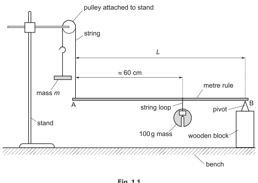
● Add masses to the mass hanger so that mass $m$ is $80\text{ g}$ .

● Adjust the pivot so that it is $5\text{ mm}$ from end B of the rule. The distance between the string at end A and the pivot is $L$ .

● Measure and record $L$ .

$L$ = ______

● Adjust the string loop supporting the $100\text{ g}$ mass so that it is approximately $60\text{ cm}$ from end A.

● Hold the rule at end A so that the rule is approximately horizontal.

● Adjust the position of the string loop to find the position where end A is just about to move upwards when the rule is released. The distance between the string at end A and the string loop is $y_1$ as shown in Fig. 1.2.

Fig. 1.2

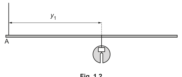
● Measure and record $y_1$ .

$y_1$ = ______

● Adjust the position of the string loop to find the position where end A is just about to move downwards when the rule is released. The distance between the string at end A and the string loop is $y_2$ .

● Measure and record $y_2$ .

$y_2$ = ______

● Calculate $y$ where

y = \frac{y_1 + y_2}{2}

$y$ = ______

DifficultyMedium-Easy

Worked solution

Working

Measure $L$ from end A (string) to pivot (set $5\ \text{mm}$ from end B).

Example readings (to nearest $1\ \text{mm}$ ):

L = 99.5\ \text{cm}

Find limiting positions of the $100\ \text{g}$ mass:

y_1 = 94.6\ \text{cm},\qquad y_2 = 94.2\ \text{cm}

Calculate

y = \frac{y_1+y_2}{2} = \frac{94.6+94.2}{2} = 94.4\ \text{cm}

Answer

$L = 99.5\ \text{cm}$ , $y_1 = 94.6\ \text{cm}$ , $y_2 = 94.2\ \text{cm}$ , $y = 94.4\ \text{cm}$ (example values; actual readings depend on the experiment).

Final answer

Example: L = 99.5 cm, y1 = 94.6 cm, y2 = 94.2 cm, y = 94.4 cm

Detailed explanation

Background Concept

In this practical you are using an equilibrium situation. When the rule is released, it will rotate one way or the other depending on whether the turning effect (moment) about the pivot is slightly clockwise or slightly anticlockwise.

Because it is hard to set the $100\ \text{g}$ mass at the exact balance point, you find two limiting positions:

one where end A is just about to move upwards (so the rotation is just about to be one way),
one where end A is just about to move downwards (just about to be the other way).

The true balance point lies between these, so the best estimate is the mean:

y = \frac{y_1+y_2}{2}.

Understanding the Question

You are told to:

set the apparatus with $m = 80\ \text{g}$ and the pivot $5\ \text{mm}$ from end B,
measure $L$ (distance from end A to the pivot),
find and measure two positions of the $100\ \text{g}$ mass, $y_1$ and $y_2$ , corresponding to “just about to move up” and “just about to move down”,
calculate the mean position $y$ .

So the marks here are for: correct measurement technique/precision and correct calculation of $y$ .

Approach

Read $L$ , $y_1$ , and $y_2$ directly from the metre rule (all as distances from end A).
Ensure each reading is to a sensible precision (typically $1\ \text{mm}$ or $0.1\ \text{cm}$ ).
Compute $y$ using the given average formula.

Step-by-Step Reasoning

Measuring $L$
- The pivot is placed close to end B (which is at the $100.0\ \text{cm}$ mark), so you expect $L$ to be close to $100\ \text{cm}$ .
- Measure from the same reference point each time: end A (where the string acts) to the pivot point.
Finding $y_1$ and $y_2$
- Slide the string loop carrying the $100\ \text{g}$ mass.
- For $y_1$ , adjust until A is just about to move upwards when released.
- For $y_2$ , adjust until A is just about to move downwards when released.
- These are two bracketing values around the true balance point.
Calculating $y$
- Use the given equation: $y = \frac{y_1+y_2}{2}.$
- Keep the final $y$ to the same resolution as $y_1$ and $y_2$ .

Key Takeaways

When the exact balance point is hard to locate, take two limiting readings and average them.
Use consistent reference points (end A here) for all distance measurements.
Record with appropriate precision for a metre rule.

Common Mistakes

Measuring $y_1$ and $y_2$ from the wrong end of the rule (must be from end A as defined).
Giving $y$ with inappropriate precision (e.g. more decimal places than the rule can justify).
Mixing units (e.g. $L$ in cm but $y$ in mm).

Things to Be Careful About

Parallax: ensure your eye is directly above the scale when reading.
Keep the rule approximately horizontal each time before release so the “just about to move” judgement is consistent.
Make sure the pivot position really is $5\ \text{mm}$ from end B; an error here affects all later results.

Techniques used

measure distances on a metre rule with appropriate precisionidentify the just-about-to-move condition in both directionscalculate the mean from two limiting readingsrecord readings with consistent units and decimal places

(b)

Increase $m$ . Measure the new values of $y_1$ and $y_2$ .

Repeat until you have five sets of values of $m$ , $y_1$ and $y_2$ .

Record your results in a table. Include values of $y$ in your table.

DifficultyMedium

Worked solution

Answer

Record at least five sets of $m$ , $y_1$ , $y_2$ and calculate $y = (y_1+y_2)/2$ each time.

Example of a suitable table (all distances from end A):

$m / \text{g}$	$y_1 / \text{cm}$	$y_2 / \text{cm}$	$y / \text{cm}$
80	94.6	94.2	94.4
100	74.7	74.3	74.5
120	54.8	54.4	54.6
140	34.9	34.5	34.7
160	15.0	14.6	14.8

(Example values; actual readings depend on the experiment.)

Final answer

See working / student-dependent table of m, y1, y2, y

Detailed explanation

Background Concept

Good experimental work needs:

enough data points (here, at least five) to establish a trend,
a sensible spread in the independent variable ( $m$ ),
repeat/limiting measurements ( $y_1$ , $y_2$ ) to reduce uncertainty in the balance position,
clear presentation in a single table with correct headings, units, and consistent precision.

The calculated value

y = \frac{y_1+y_2}{2}

should be derived from the two bracketing readings for each mass.

Understanding the Question

You must increase $m$ several times and, for each $m$ :

measure $y_1$ (just about to move up),
measure $y_2$ (just about to move down),
calculate $y$ ,
then present the results in a table.

The marks are for: enough sets, clear table layout, correct unit headings, and correctly calculated $y$ values.

Approach

Choose a set of $m$ values (e.g. increasing in equal steps) giving a good range.
For each $m$ , repeat the same bracketing procedure used in (a) to get $y_1$ and $y_2$ .
Immediately calculate $y$ and enter it in the table.
Keep decimal places consistent within each column (e.g. all $y$ values to $0.1\ \text{cm}$ ).

Step-by-Step Reasoning

Select values of $m$
Use at least five distinct masses, increasing from the initial $80\ \text{g}$ . Equal steps help the graph later.
Measure $y_1$ and $y_2$ for each $m$
- Keep the pivot position fixed.
- Keep the method consistent: rule approximately horizontal before release.
- Record both limiting readings.
Compute $y$
For each row:
$y = \frac{y_1+y_2}{2}.$
If $y_1$ and $y_2$ are to $0.1\ \text{cm}$ , quote $y$ to $0.1\ \text{cm}$ .
Construct the table
- One table only.
- Column headings must contain quantity and unit (e.g. $y_1 / \text{cm}$ ).
- Numerical entries aligned and consistent dp.

Key Takeaways

Collect enough points and a suitable range to justify drawing a straight line.
Use bracketing readings to reduce judgement error in “balance point”.
Present raw and derived data clearly and consistently.

Common Mistakes

Fewer than five sets of readings.
Missing units in table headings.
Inconsistent decimal places within a column.
Calculating $y$ incorrectly (e.g. $y_1-y_2$ instead of mean).

Things to Be Careful About

Don’t change the pivot position while changing $m$ .
Ensure $m$ is the total mass on the hanger (including the hanger if instructed).
Record $y_1$ and $y_2$ as distances from end A, not from the pivot.

Techniques used

vary the independent variable over a suitable rangerepeat the bracketing method to obtain limiting readingsrecord raw and derived quantities in a single table with unitscalculate a derived mean value for each run

(c)

(i)

Plot a graph of $y$ on the $y$ -axis against $m$ on the $x$ -axis.

DifficultyMedium-Easy

Worked solution

Answer

Plot $y$ (vertical axis) against $m$ (horizontal axis).

Label axes as $y / \text{cm}$ and $m / \text{g}$ (or the units used in the table).
Use a suitable scale (at least half the grid on each axis).
Plot all five points accurately.

Final answer

Graph of y against m plotted with correct axes, units, scale, and points

Detailed explanation

Background Concept

A graph helps you test whether two variables are linearly related. If $y$ and $m$ satisfy

y = Am + B,

then a plot of $y$ against $m$ should be a straight line.

To gain marks in Paper 3, you must show good graphing technique: correct labels, sensible scales, accurate plotting.

Understanding the Question

You are asked specifically to put $y$ on the $y$ -axis and $m$ on the $x$ -axis. That means $m$ is treated as the independent variable (what you changed) and $y$ as the dependent variable (what you measured/calculated).

Approach

Decide the ranges from your table (minimum and maximum of $m$ and $y$ ).
Choose axis scales that are easy to use (1, 2, 5, 10 etc. per major square).
Label each axis with both symbol and unit.
Plot points with small, neat crosses.

Step-by-Step Reasoning

Axes and labels
- Horizontal axis: $m$ with its unit.
- Vertical axis: $y$ with its unit.
Scale choice
- Use most of the available grid area.
- Avoid awkward scales (e.g. 3 per square) because they reduce accuracy.
Plotting
- Plot each point precisely using a ruler.
- Make the plotted symbols clear but not oversized.

Key Takeaways

Independent variable on $x$ -axis; dependent variable on $y$ -axis.
Labels must include units.
Good scales and accurate plotting are assessed.

Common Mistakes

Axes swapped (plotting $m$ on the $y$ -axis).
Missing units on axes.
Using a tiny part of the grid (poor scale choice).
Plotting blobs instead of neat crosses.

Things to Be Careful About

Ensure the plotted values match the table exactly.
If your $y$ values decrease as $m$ increases, the graph will slope downwards; that is fine if it matches the data.

Techniques used

choose suitable axis scales that use most of the graph paperlabel axes with quantity and unitplot experimental points accuratelyuse consistent plotting conventions for points

(ii)

Draw the straight line of best fit.

DifficultyEasy

Worked solution

Answer

Draw one straight line of best fit through the plotted points with an approximately even distribution of points on either side of the line.

Final answer

Straight line of best fit drawn

Detailed explanation

Background Concept

A best-fit line represents the overall linear trend in the data. Because experimental points have scatter, the line should not be forced through every point.

Understanding the Question

After plotting the points in (c)(i), you must draw the straight line that best represents the trend.

Approach

Use a ruler.
Position the line so that the deviations of points above and below are balanced.
Do not join the dots.

Step-by-Step Reasoning

Place a ruler so the line follows the general trend of the points.
Adjust so roughly equal numbers of points lie above and below.
Draw a single, thin straight line across the full span of your data.

Key Takeaways

Best-fit means balanced scatter, not necessarily passing through all points.

Common Mistakes

Joining points dot-to-dot.
Forcing the line through the origin without evidence.
Drawing a thick line that makes reading gradient/intercept inaccurate.

Things to Be Careful About

If one point is a clear anomaly, the best-fit line may reasonably not pass close to it, but you still plot it.

Techniques used

draw a single straight best-fit line with balanced scatteravoid point-to-point joiningextend the line appropriately across the data range

(iii)

Determine the gradient and $y$ -intercept of this line.

gradient = ______

$y$ -intercept = ______

DifficultyMedium

Worked solution

Working

Using two well-separated points on the best-fit line (example):

(m_1, y_1) = (80\ \text{g},\ 94.4\ \text{cm}),\qquad (m_2, y_2) = (160\ \text{g},\ 14.8\ \text{cm})

Gradient:

\text{gradient} = \frac{\Delta y}{\Delta m} = \frac{14.8-94.4}{160-80} = \frac{-79.6}{80} = -0.995\ \text{cm g}^{-1}

$y$ -intercept (using $y = (\text{gradient})\,m + c$ ):

c = y - (\text{gradient})\,m = 94.4 - (-0.995)(80) = 174\ \text{cm}

Answer

gradient $= -0.995\ \text{cm g}^{-1}$

$y$ -intercept $= 174\ \text{cm}$

(example values; depend on candidate’s graph)

Final answer

Example: gradient = −0.995 cm g⁻¹, y-intercept = 174 cm

Detailed explanation

Background Concept

For a straight-line graph of $y$ (vertical) against $m$ (horizontal), the gradient is

\text{gradient} = \frac{\Delta y}{\Delta m}

and the $y$ -intercept is the value of $y$ when $m = 0$ .

In the linear form

y = Am + B,

$A$ is the gradient and $B$ is the $y$ -intercept.

Understanding the Question

You must read two quantities from your best-fit line:

the gradient (slope),
the intercept where the line crosses the $y$ -axis.

These will be used in later parts to find constants, so accuracy matters.

Approach

Choose two points on the line, not necessarily data points.
Make the points far apart to reduce percentage uncertainty.
Calculate gradient as “rise over run” = change in $y$ divided by change in $m$ .
Read the $y$ -intercept directly where the line meets the $y$ -axis (or compute it using $y = mx + c$ with one point).

Step-by-Step Reasoning

Pick two points on the best-fit line
Using widely separated values (near the ends of the line) gives a large triangle, which improves accuracy.
Compute the gradient
- Work out $\Delta y$ (vertical change) and $\Delta m$ (horizontal change).
- Divide: $\text{gradient} = \frac{\Delta y}{\Delta m}.$
- Keep the sign: if $y$ decreases as $m$ increases, the gradient is negative.
Find the intercept
- Either read it from the graph at $m=0$ , or use $c = y - (\text{gradient})\,m$ with a point $(m,y)$ on the best-fit line.
Quote units
- If $y$ is in cm and $m$ in g, gradient units are $\text{cm g}^{-1}$ and intercept units are cm.

Key Takeaways

Use a large triangle to reduce uncertainty in gradient.
Gradient is always $\Delta y/\Delta x$ (here $\Delta y/\Delta m$ ).
Intercept is the value at $m=0$ (even if it lies off the plotted range).

Common Mistakes

Using two neighbouring points, giving an inaccurate gradient.
Calculating $\Delta m/\Delta y$ instead of $\Delta y/\Delta m$ .
Using data points rather than points on the best-fit line.
Forgetting the negative sign for a downward-sloping line.

Things to Be Careful About

Ensure both points used for the gradient are actually on the drawn line.
Read coordinates carefully from the axes and include units.

Techniques used

use a large triangle to determine the gradientcalculate the gradient as $\Delta y / \Delta x$determine the y-intercept from the best-fit lineuse consistent units when quoting gradient and intercept

(d)

It is suggested that the quantities $y$ and $m$ are related by the equation

y = Am + B

where $A$ and $B$ are constants.

Using your answers in (c)(iii), determine the values of $A$ and $B$ .
Give appropriate units.

$A$ = ______

$B$ = ______

DifficultyMedium-Easy

Worked solution

Answer

From $y = Am + B$ and the graph of $y$ against $m$ :

A = \text{gradient},\qquad B = y\text{-intercept}

Using (c)(iii) (example):

A = -0.995\ \text{cm g}^{-1},\qquad B = 174\ \text{cm}

Final answer

Example: A = −0.995 cm g⁻¹, B = 174 cm

Detailed explanation

Background Concept

A straight line has the general form

y = mx + c.

If you plot $y$ against $m$ and obtain a straight line, then comparing with

y = Am + B

shows that:

$A$ plays the role of the gradient,
$B$ plays the role of the $y$ -intercept.

Units follow directly from the plotted quantities.

Understanding the Question

You are told the suggested relation is $y = Am + B$ and you have already found the gradient and intercept from your graph. You now just state $A$ and $B$ equal to those values, with appropriate units.

Approach

Set $A$ equal to your gradient.
Set $B$ equal to your $y$ -intercept.
Assign units: $A$ has units of $y$ per $m$ ; $B$ has the same units as $y$ .

Step-by-Step Reasoning

If $y$ is plotted on the vertical axis and $m$ on the horizontal axis, then $A = \frac{\Delta y}{\Delta m}.$
The intercept at $m=0$ is $B$ .
If your axes were $y / \text{cm}$ and $m / \text{g}$ , then $[A] = \text{cm g}^{-1},\qquad [B] = \text{cm}.$

Key Takeaways

On a $y$ vs $m$ graph, gradient corresponds to the coefficient of $m$ .
Intercept corresponds to the constant term.
Units come from the axes.

Common Mistakes

Swapping $A$ and $B$ .
Giving $B$ the wrong units (it must match $y$ ).
Forgetting that a downward slope means negative $A$ .

Things to Be Careful About

Use the same units as your graph/table. If you plotted $m$ in kg, then $A$ would be in $\text{cm kg}^{-1}$ (or $\text{m kg}^{-1}$ depending on $y$ units).

Techniques used

match a straight-line graph to the form $y=mx+c$identify constants from gradient and interceptstate appropriate units for derived constants

(e)

Theory suggests that

B = L - \frac{RA}{2}

where $R$ is the mass of the metre rule.

Determine a value for $R$ .
Give your answer to three significant figures.

$R$ = ______

DifficultyMedium

Worked solution

Working

Given

B = L - \frac{RA}{2}

Rearrange:

\frac{RA}{2} = L - B \;\Rightarrow\; R = \frac{2(L-B)}{A}

Using $L = 99.5\ \text{cm}$ from (a), and (example) $A = -0.995\ \text{cm g}^{-1}$ , $B = 174\ \text{cm}$ :

R = \frac{2(99.5-174)}{-0.995} = \frac{2(-74.5)}{-0.995} = 1.50 \times 10^2\ \text{g}

Answer

R = 150\ \text{g}\ \text{(3 s.f.)}

Final answer

R = 150 g

Detailed explanation

Background Concept

When experimental data give a straight line $y = Am + B$ , the constants $A$ and $B$ can be used in a theoretical relationship to determine another physical quantity. Here the theory links the intercept $B$ to the distance $L$ , the gradient $A$ , and the mass $R$ of the metre rule:

B = L - \frac{RA}{2}.

If you know $A$ , $B$ , and $L$ , you can solve for $R$ .

diagram-e1

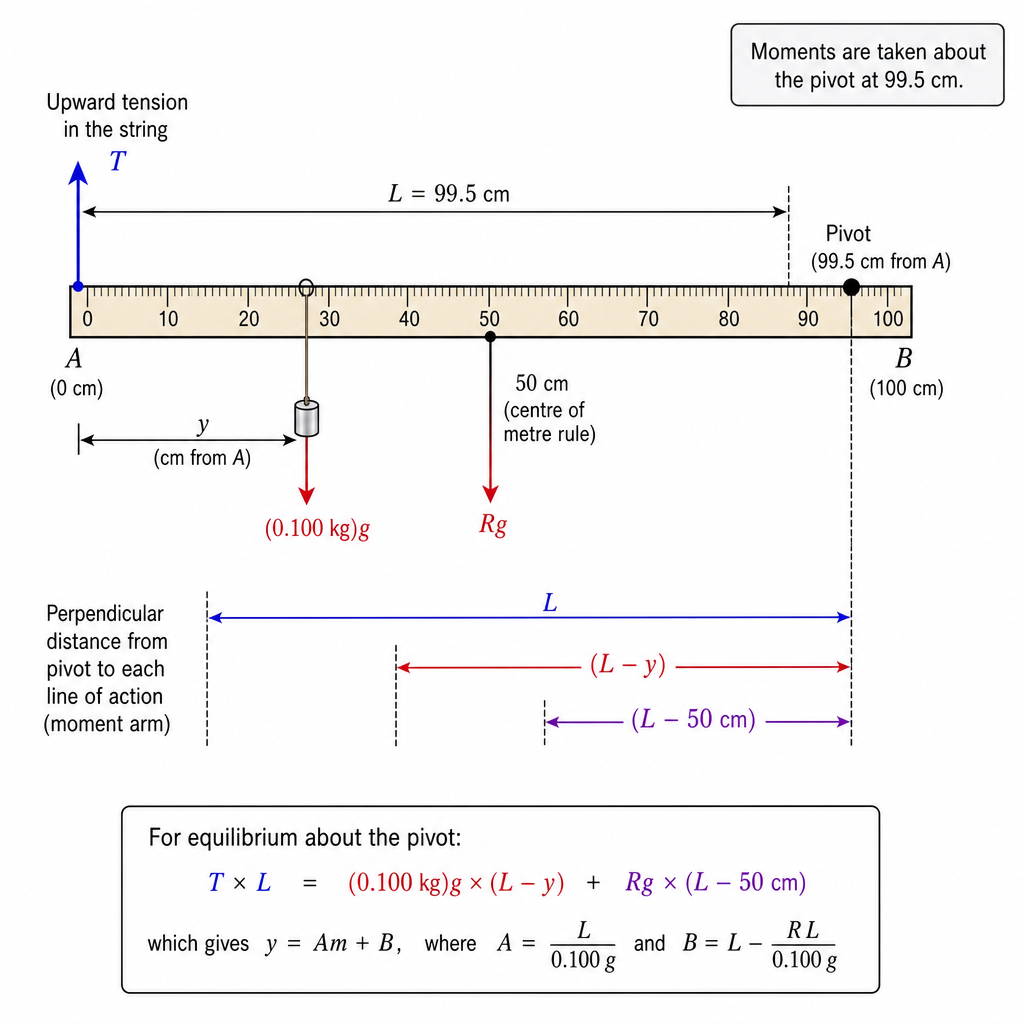
Understanding the Question

You are given the theoretical equation

B = L - \frac{RA}{2}

and asked to determine $R$ (mass of the metre rule), using your values of $A$ and $B$ from the graph and your measured $L$ .

The instruction “three significant figures” applies to the final numerical value of $R$ .

Approach

Rearrange the equation to make $R$ the subject.
Substitute the measured/graph values.
Keep track of signs: if $A$ is negative, the division will change sign.
Quote $R$ to 3 s.f. with units consistent with the units used for $A$ , $B$ , and $L$ .

Step-by-Step Reasoning

Start with
$B = L - \frac{RA}{2}.$
Move terms to isolate the $RA$ term:
$\frac{RA}{2} = L - B.$
Make $R$ the subject:
$R = \frac{2(L-B)}{A}.$
Substitute your values. For example, with $L=99.5\ \text{cm}$ , $B=174\ \text{cm}$ and $A=-0.995\ \text{cm g}^{-1}$ :
- Compute $L-B = 99.5-174 = -74.5\ \text{cm}$ .
- Then $R = \frac{2(-74.5)}{-0.995}\ \text{g} \approx 150\ \text{g}.$
The negatives cancel, giving a positive mass as expected.
Units check
If $L$ and $B$ are in cm, then $(L-B)$ is in cm. If $A$ is in $\text{cm g}^{-1}$ , then dividing cm by $\text{cm g}^{-1}$ gives g, so $R$ comes out in grams.

Key Takeaways

Rearranging a linear-theory equation is a standard way to extract a physical constant from a graph.
Always check the sign: masses must be positive.
Units must be consistent across $L$ , $B$ , and $A$ .

Common Mistakes

Rearrangement error: writing $R = 2A(L-B)$ instead of dividing by $A$ .
Forgetting that $A$ may be negative, leading to a negative $R$ (which is unphysical).
Mixing cm and m (e.g. using $L$ in cm but $B$ in m).
Not giving $R$ to three significant figures.

Things to Be Careful About

Use the same units as your graph. If you plotted $m$ in kg, then $A$ will have different units and $R$ will come out in kg.
Intercepts may be outside the plotted range; that is normal for extrapolation, but it makes accurate gradient/intercept measurement important.

Techniques used

rearrange an equation to make the target variable the subjectsubstitute experimental constants into the rearranged equationcheck and state significant figures and units

The rest of this paper

1 more questions

Q2Manipulation, Measurement and Observation · Analysis, Conclusions and Evaluation · Presentation of Data and Observations20M

Loading the full paper…