Physics 9702/32 — May/June 2020

Cambridge AS Level · Advanced Practical Skills · worked solutions for every part, with the mark scheme

questions

marks

120

minutes

Topics Manipulation, Measurement and Observation · Presentation of Data and Observations · Analysis, Conclusions and Evaluation

Q1Manipulation, Measurement and ObservationPresentation of Data and ObservationsAnalysis, Conclusions and EvaluationFree sample

In this experiment, you will investigate a pendulum made from a wooden strip with masses fixed at one end.

(a)

Some of the apparatus has been assembled for you.

● Pass the nail through the hole in the strip furthest from the masses.
● Fix the nail securely in the clamp.
● Complete the set-up of the apparatus as shown in Fig. 1.1.

Fig. 1.1

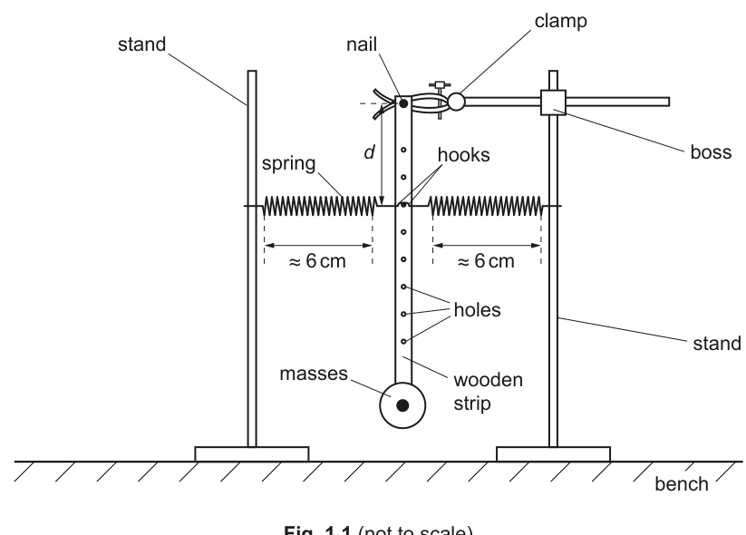
● The hooks at the ends of the springs should pass through one of the holes in the strip.
Position the stands so that the coiled section of each spring is of approximate length 6 cm and the strip is vertical.
● The distance along the strip between the nail and the hole with the hooks is $d$ .
Measure and record $d$ .

$d$ = ______ $\text{cm}$

DifficultyEasy

Worked solution

Answer

Measure $d$ along the strip from the centre of the nail hole to the centre of the hole used for the hooks, using a ruler.

Recorded value (to nearest $0.1\ \text{cm}$ ):

d = 18.6\ \text{cm}

Final answer

d = 18.6 cm

Detailed explanation

Background Concept

In practical work, a length measurement should be:

taken between clearly defined reference points,
made with an appropriate instrument (here, a ruler),
recorded with suitable precision (typically to the nearest millimetre, i.e. $0.1\ \text{cm}$ ), and
always written with a unit.

Understanding the Question

You are told that $d$ is the distance along the strip between the nail position (pivot) and the hole where the spring hooks are attached. You must measure this distance and record it in $\text{cm}$ .

Approach

Decide the two endpoints of $d$ (centre-to-centre of the relevant holes).
Place the ruler along the strip and read the distance without parallax.
Record the reading with a unit and appropriate precision.

Step-by-Step Reasoning

Identify the pivot point: the nail passes through a hole near the top of the strip.
Identify the hook hole: the hole through which both spring hooks pass.
Place the ruler along the strip so that it follows the strip (not a slanted line in space).
Read from the centre of the nail hole to the centre of the hook hole.
Record to $0.1\ \text{cm}$ (ruler resolution $= 1\ \text{mm}$ ).

Example of a correctly recorded measurement:

d = 18.6\ \text{cm}

Key Takeaways

Measure the correct quantity (centre-to-centre between the specified holes).
Avoid parallax and record with correct precision and unit.

Common Mistakes

Measuring from the top of the strip rather than from the nail hole.
Measuring to the edge of a hole rather than the centre.
Recording with no unit or with unrealistic precision (e.g. $18.63\ \text{cm}$ on a ruler).

Things to Be Careful About

Ensure the ruler is aligned along the strip.
Read at eye level to avoid parallax.
Use consistent units: the question asks for $d$ in $\text{cm}$ .

Techniques used

identify the correct points between which the length is measureduse a ruler to take a length reading with appropriate precisionrecord a measurement with a unit and sensible significant figures

(b)

● Move the bottom of the strip towards one of the stands and release it so that it oscillates.
● Take measurements to determine the period $T$ of these oscillations.

$T$ = ______ $\text{s}$

DifficultyMedium-Easy

Worked solution

Working

Time $N = 10$ oscillations twice.

Example readings:

t_1(10T) = 12.40\ \text{s},\quad t_2(10T) = 12.36\ \text{s}

Mean time for $10T$ :

\overline{t}(10T) = \frac{12.40 + 12.36}{2} = 12.38\ \text{s}

Period:

T = \frac{\overline{t}(10T)}{10} = \frac{12.38}{10} = 1.238\ \text{s} \approx 1.24\ \text{s}

Answer

T = 1.24\ \text{s}

Final answer

T = 1.24 s

Detailed explanation

Background Concept

The period $T$ is the time for one complete oscillation. Using a handheld stopwatch, the main uncertainty is human reaction time, so a better method is:

time several oscillations (e.g. $N = 10$ or $20$ ), then
divide the total time by $N$ .
Repeating the timing and averaging reduces random error.

Understanding the Question

You set the strip oscillating and must determine the period $T$ . The question awards marks for an appropriate measurement method, not a specific numerical value (since your period depends on your apparatus and how far you displaced the strip).

Approach

Choose a number of oscillations $N$ (at least 10 is standard).
Use a fixed reference point and count oscillations consistently.
Repeat the timing at least once.
Average and divide by $N$ to obtain $T$ .

Step-by-Step Reasoning

Start the oscillation with a small, consistent displacement.
Pick a reference position (e.g. when the bottom of the strip passes the centre line).
Start the stopwatch as the strip passes the reference position.
Count 10 complete oscillations (returning to the same position and direction counts one oscillation).
Stop the stopwatch on the 10th return.
Repeat to get a second value.
Average the two totals, then divide by 10.

Example:

$t_1(10T) = 12.40\ \text{s}$ , $t_2(10T) = 12.36\ \text{s}$
Mean $= 12.38\ \text{s}$
$T = 12.38/10 = 1.238\ \text{s} \approx 1.24\ \text{s}$

Key Takeaways

Timing many oscillations reduces fractional uncertainty.
Repeats and averaging improve reliability.

Common Mistakes

Timing only one oscillation (large percentage uncertainty).
Counting half-oscillations as full oscillations.
Starting/stopping at different points in the motion each time.

Things to Be Careful About

Keep the amplitude small and similar each time (large amplitudes can slightly change the period).
Use the same reference point and count method for every run.
Quote $T$ to a sensible precision (typically $0.01\ \text{s}$ if derived from a stopwatch reading to $0.01\ \text{s}$ ).

Techniques used

time multiple oscillations and divide to obtain the periodrepeat measurements and average to improve reliabilityuse a stopwatch with appropriate resolution

(c)

Move the hooks to a different hole in the strip. Measure $d$ and $T$ . Repeat until you have six sets of values of $d$ and $T$ .

Record your results in a table. Include values of $d^2$ and $\frac{1}{T^2}$ in your table.

DifficultyMedium

Worked solution

Answer

Record six sets of $d$ and $T$ (repeating timings and averaging). Calculate $d^2$ and $\dfrac{1}{T^2}$ .

Example of a correctly presented table (headings include units; consistent precision):

$d / \text{cm}$	$T / \text{s}$	$d^2 / \text{cm}^2$	$1/T^2 / \text{s}^{-2}$
10.0	1.83	100	0.299
12.0	1.70	144	0.346
15.0	1.53	225	0.427
18.0	1.38	324	0.526
22.0	1.21	484	0.685
28.0	1.01	784	0.980

(Values shown are illustrative; your measured values may differ.)

Final answer

See table (six sets of d, T with calculated d^2 and 1/T^2)

Detailed explanation

Background Concept

A good results table in Paper 3 must:

contain all raw and derived data in one table,
have clear column headings with quantity / unit (e.g. $d / \text{cm}$ ),
use a consistent number of decimal places for the same measured quantity,
include a sufficient range of the independent variable (here $d$ ), and
include correctly calculated derived quantities (here $d^2$ and $1/T^2$ ).

Understanding the Question

You must move the hooks to different holes, so $d$ changes. For each $d$ , you measure the oscillation period $T$ . You need six sets of $(d, T)$ and then calculate and record $d^2$ and $1/T^2$ .

Approach

Choose six different holes giving a good spread of $d$ values.
For each $d$ $d$ :
- measure $d$ with a ruler,
- time $N$ oscillations at least twice, average, and divide by $N$ to get $T$ .
Calculate $d^2$ and $1/T^2$ for each row.
Present everything in one table with correct headings/units and consistent precision.

Step-by-Step Reasoning

Independent variable: $d$ (you change this by choosing different holes).
Dependent variable: $T$ (you measure the resulting oscillations).
After measuring $d$ (typically to $0.1\ \text{cm}$ ), square it to obtain $d^2$ in $\text{cm}^2$ .
After finding $T$ (typically to $0.01\ \text{s}$ ), compute:

\frac{1}{T^2}

and record it in $\text{s}^{-2}$ .

Example calculation for one row (if $T = 1.70\ \text{s}$ ):

\frac{1}{T^2} = \frac{1}{(1.70)^2} = \frac{1}{2.89} = 0.346\ \text{s}^{-2}

A table that would score well includes:

at least 6 rows,
headings like $d / \text{cm}$ , $T / \text{s}$ , $d^2 / \text{cm}^2$ , $1/T^2 / \text{s}^{-2}$ ,
consistent d.p. down columns (e.g. all $d$ to 1 d.p., all $T$ to 2 d.p.).

Key Takeaways

Collect enough data points with a good spread in $d$ .
Derived columns must be calculated correctly and labelled with units.
Consistent presentation is assessed.

Common Mistakes

Fewer than six sets of readings.
Missing units in headings (e.g. writing just $d$ rather than $d/\text{cm}$ ).
Mixing decimal places in a column without reason.
Calculating $1/T$ instead of $1/T^2$ .
Forgetting that $d^2$ has units of $\text{cm}^2$ .

Things to Be Careful About

Keep the oscillation amplitude similar for each run.
When squaring, do not round too early; round at the end of the calculation.
Make sure the derived values are consistent with the measured precision (don’t quote excessive significant figures).

Techniques used

collect multiple paired readings over a suitable range of the independent variablecalculate derived quantities from measured dataconstruct a results table with headings that include quantities and unitsuse consistent significant figures and decimal places down each column

(d)

(i)

Plot a graph of $\frac{1}{T^2}$ on the $y$ -axis against $d^2$ on the $x$ -axis.

DifficultyMedium-Easy

Worked solution

Answer

Plot a graph with:

$x$ -axis: $d^2 / \text{cm}^2$
$y$ -axis: $1/T^2 / \text{s}^{-2}$
sensible scales using at least half the graph paper in each direction
all six points plotted accurately as small crosses.

Final answer

Graph of 1/T^2 (y) against d^2 (x) plotted with labelled axes and suitable scales

Detailed explanation

Background Concept

A good experimental graph should:

have axes labelled with quantity and unit,
use a linear scale with convenient intervals,
use most of the available grid,
plot points accurately (small, neat crosses), and
match the variables requested (here $y = 1/T^2$ against $x = d^2$ ).

Understanding the Question

You have calculated $d^2$ and $1/T^2$ in your table. You must plot $1/T^2$ on the vertical axis and $d^2$ on the horizontal axis. The purpose is to check for a straight-line relationship.

Approach

Decide the range of $d^2$ and $1/T^2$ from your table.
Choose scales so the plotted points spread across the graph (not bunched in a corner).
Label axes with correct symbols and units.
Plot all points carefully.

Step-by-Step Reasoning

Put $d^2$ on the $x$ -axis because it is the controlled/independent variable.
Put $1/T^2$ on the $y$ -axis.
Example axis labels:
- horizontal: $d^2 / \text{cm}^2$
- vertical: $1/T^2 / \text{s}^{-2}$
Use a scale like 1 large square = 50 or 100 $\text{cm}^2$ (depending on your range) so the points cover at least half the width.
Plot each pair $(d^2, 1/T^2)$ as a small cross.

Key Takeaways

Correct axes, units, and good use of the grid are as important as the points themselves.

Common Mistakes

Swapping axes (plotting $d^2$ on $y$ ).
Missing units in labels.
Awkward scales (e.g. 1 large square = 3 units) that waste grid space.
Plotting dots so large they hide the best-fit line.

Things to Be Careful About

Ensure you are plotting $d^2$ and not $d$ .
Ensure you are plotting $1/T^2$ and not $T^2$ .
Check each plotted point against the table before drawing any line.

Techniques used

choose sensible axis scales that use most of the gridlabel axes with quantity and unitplot experimental points accurately

(ii)

Draw the straight line of best fit.

DifficultyEasy

Worked solution

Answer

Draw a single straight line of best fit through the plotted points, with the scatter of points approximately balanced about the line.

Final answer

Straight line of best fit drawn

Detailed explanation

Background Concept

A line of best fit represents the trend suggested by the data when random errors cause scatter. For a linear relationship, you draw one straight line so that points are roughly evenly distributed above and below it.

Understanding the Question

After plotting the six points, you must draw the straight line that best represents the relationship between $1/T^2$ and $d^2$ .

Approach

Use a ruler.
Do not connect point-to-point.
Aim for a line that leaves roughly equal numbers of points on each side (allowing for error).

Step-by-Step Reasoning

Place the ruler so the line passes centrally through the cluster of points.
If one point is clearly anomalous (far from the trend), do not force the line through it; keep the best overall balance.
Draw the line across most of the plotted range (not just between two middle points).

Key Takeaways

Best-fit means overall trend, not exact passage through every point.

Common Mistakes

Joining points with segments.
Forcing the line through the origin when not justified.
Drawing a line that follows one extreme point rather than the general trend.

Things to Be Careful About

Use a sharp pencil so the line is thin.
Extend the line enough so that intercept readings are possible.

Techniques used

draw a straight line of best fit with balanced scatteravoid join-the-dots and ignore minor random deviations

(iii)

Determine the gradient and $y$ -intercept of this line.

gradient = ______
$y$ -intercept = ______

DifficultyMedium-Easy

Worked solution

Working

Using two points on the best-fit line, e.g.

(d^2,\ 1/T^2) = (100\ \text{cm}^2,\ 0.30\ \text{s}^{-2})\ \text{and}\ (784\ \text{cm}^2,\ 0.98\ \text{s}^{-2})

Gradient:

\text{gradient} = \frac{\Delta y}{\Delta x} = \frac{0.98 - 0.30}{784 - 100} = \frac{0.68}{684} = 9.9 \times 10^{-4}\ \text{s}^{-2}\ \text{cm}^{-2}

$y$ -intercept (using $y = mx + c$ ):

c = 0.30 - (9.9 \times 10^{-4})\times 100 \approx 0.20\ \text{s}^{-2}

Answer

\text{gradient} = 9.9 \times 10^{-4}\ \text{s}^{-2}\ \text{cm}^{-2}

y\text{-intercept} = 0.20\ \text{s}^{-2}

Final answer

gradient = 9.9 × 10^-4 s^-2 cm^-2, y-intercept = 0.20 s^-2

Detailed explanation

Background Concept

For a straight-line graph of $y$ against $x$ :

y = mx + c

the gradient is $m = \Delta y / \Delta x$ (change in $y$ divided by change in $x$ ),
the $y$ -intercept is $c$ , the value of $y$ when $x = 0$ .

In experiments, you should calculate gradient from the best-fit line, not from two adjacent data points, and you should use a large triangle to reduce percentage reading error.

Understanding the Question

You plotted $y = 1/T^2$ against $x = d^2$ and drew a best-fit straight line. Now you must find:

the gradient of that line, and
the $y$ -intercept.

These will be used in part (e).

Approach

Choose two points on the best-fit line that are far apart (widely separated in $x$ ).
Read their coordinates accurately.
Compute $m = \Delta y/\Delta x$ .
Find the intercept either by reading where the line crosses the $y$ -axis, or by using $c = y - mx$ .

Step-by-Step Reasoning

diagram-1

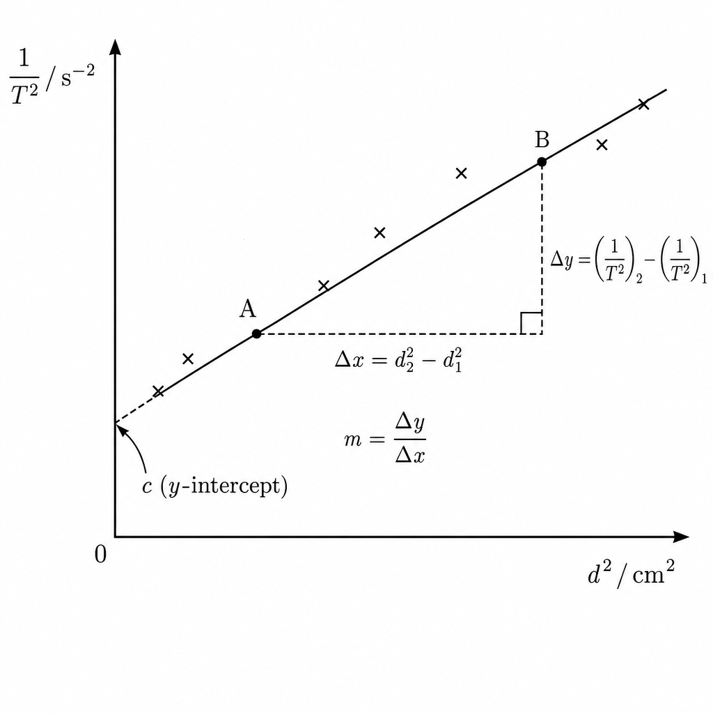
Pick two clear points on the drawn line, ideally near the ends of the plotted range.
Suppose the chosen points are $(x_1, y_1)$ and $(x_2, y_2)$ .
Compute:

\Delta y = y_2 - y_1,\quad \Delta x = x_2 - x_1

and then:

m = \frac{\Delta y}{\Delta x}

Units: here $y$ has units $\text{s}^{-2}$ and $x$ has units $\text{cm}^2$ , so:

[m] = \frac{\text{s}^{-2}}{\text{cm}^2} = \text{s}^{-2}\ \text{cm}^{-2}

For the intercept, either read $y$ when $x=0$ from the graph, or use:

c = y_1 - mx_1

and the unit of $c$ is the same as $y$ , i.e. $\text{s}^{-2}$ .

Key Takeaways

Gradient must come from the line, using a large triangle.
Always include correct units for gradient and intercept.

Common Mistakes

Using two data points that are not on the best-fit line.
Using a tiny triangle (large percentage uncertainty).
Inverting the gradient (doing $\Delta x / \Delta y$ ).
Giving no units, or incorrect units (e.g. $\text{s}^{-2}\ \text{cm}^2$ ).

Things to Be Careful About

Read coordinates carefully from the axes and scale.
Keep enough significant figures during calculation; round sensibly at the end.
If reading the intercept by extrapolation, extend the line cleanly and thinly to the $y$ -axis.

Techniques used

select two well-separated points on the best-fit linecalculate gradient using $\Delta y / \Delta x$determine y-intercept by extrapolation or substitution

(e)

It is suggested that the quantities $T$ and $d$ are related by the equation

\frac{1}{T^2} = ad^2 + b

where $a$ and $b$ are constants.

Use your answers in (d)(iii) to determine the values of $a$ and $b$ .
Give appropriate units.

$a$ = ______
$b$ = ______

DifficultyMedium-Easy

Worked solution

Working

Given:

\frac{1}{T^2} = ad^2 + b

Comparing with $y = mx + c$ for a graph of $y = 1/T^2$ against $x = d^2$ :

a = \text{gradient},\quad b = y\text{-intercept}

Using (d)(iii):

a = 9.9 \times 10^{-4}\ \text{s}^{-2}\ \text{cm}^{-2}

b = 0.20\ \text{s}^{-2}

Answer

a = 9.9 \times 10^{-4}\ \text{s}^{-2}\ \text{cm}^{-2}

b = 0.20\ \text{s}^{-2}

Final answer

a = 9.9 × 10^-4 s^-2 cm^-2, b = 0.20 s^-2

Detailed explanation

Background Concept

If a relationship can be written as:

y = mx + c

then a plot of $y$ (vertical) against $x$ (horizontal) is a straight line with:

gradient $m$
y-intercept $c$

Here the proposed equation is:

\frac{1}{T^2} = ad^2 + b

So it already matches the straight-line form if we identify:

y = \frac{1}{T^2},\quad x = d^2

Understanding the Question

You have already found the gradient and y-intercept from your graph of $1/T^2$ vs $d^2$ . This part asks you to use those values to determine the constants $a$ and $b$ , including appropriate units.

Approach

Match the given equation to $y = mx + c$ .
Set $a$ equal to the gradient and $b$ equal to the y-intercept.
Determine units using the axes:
- $1/T^2$ has units $\text{s}^{-2}$ ,
- $d^2$ has units $\text{cm}^2$ (since you measured $d$ in cm),
- therefore $a$ has units $\text{s}^{-2}\ \text{cm}^{-2}$ and $b$ has units $\text{s}^{-2}$ .

Step-by-Step Reasoning

Start from:

\frac{1}{T^2} = ad^2 + b

Compare with $y = mx + c$ :

y \equiv \frac{1}{T^2},\quad x \equiv d^2

So:

a \equiv m\ (\text{gradient}),\quad b \equiv c\ (y\text{-intercept})

Units:

\left[\frac{1}{T^2}\right] = \text{s}^{-2},\quad [d^2] = \text{cm}^2

Therefore:

[a] = \frac{\text{s}^{-2}}{\text{cm}^2} = \text{s}^{-2}\ \text{cm}^{-2},\quad [b] = \text{s}^{-2}

Substitute your measured gradient and intercept from (d)(iii) to obtain the numerical values of $a$ and $b$ .

Key Takeaways

When your graph is $y$ against $x$ , the gradient gives the coefficient of $x$ .
The intercept gives the constant term.
Units come directly from axis units.

Common Mistakes

Swapping $a$ and $b$ .
Giving $a$ the same units as $b$ (forgetting that $a$ multiplies $d^2$ ).
Using $d$ rather than $d^2$ when stating units.

Things to Be Careful About

If you measured $d$ in $\text{cm}$ , then $d^2$ is in $\text{cm}^2$ , not $\text{m}^2$ .
Keep your unit statement consistent with what you actually plotted on the axes.

Techniques used

match a straight-line graph to the form y = mx + cidentify constants from gradient and interceptdeduce correct units from axis units

The rest of this paper

1 more questions

Q2Manipulation, Measurement and Observation · Analysis, Conclusions and Evaluation · Presentation of Data and Observations20M

Loading the full paper…