In this experiment, you will investigate the equilibrium of a loaded wooden strip. (i) • Balance the wooden strip on the prism. • Use the pencil to make a small line on the side of the wooden strip where it touches the prism, as shown in Fig. 1.1. • Roll the piece of modelling clay into a uniform cylinder of approximate length 20 cm and place it on the wooden strip with one end above the line, as shown in Fig. 1.2. • Place the mass on the wooden strip and adjust the position…

Physics 9702/36 — October/November 2019

Cambridge AS Level · Advanced Practical Skills · worked solutions for every part, with the mark scheme

questions

marks

120

minutes

Topics Manipulation, Measurement and Observation · Presentation of Data and Observations · Analysis, Conclusions and Evaluation

Q1Manipulation, Measurement and ObservationPresentation of Data and ObservationsAnalysis, Conclusions and EvaluationFree sample

In this experiment, you will investigate the equilibrium of a loaded wooden strip.

(a)

(i)

• Balance the wooden strip on the prism.
• Use the pencil to make a small line on the side of the wooden strip where it touches the prism, as shown in Fig. 1.1.

Fig. 1.1

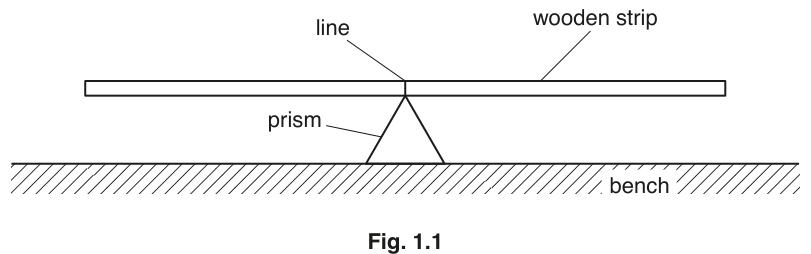
• Roll the piece of modelling clay into a uniform cylinder of approximate length 20 cm and place it on the wooden strip with one end above the line, as shown in Fig. 1.2.
• Place the mass on the wooden strip and adjust the position of the mass until the strip balances, as shown in Fig. 1.2.

Fig. 1.2

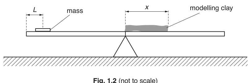
• The length of the cylinder of modelling clay is $x$ , as shown in Fig. 1.2.

Measure and record $x$ .

$x$ = ______ $\text{cm}$

DifficultyEasy

Worked solution

Measure $x$ with a ruler to the nearest $1\ \text{mm}$ .

Example reading:

x = 20.0\ \text{cm}

Final answer

x = 20.0 cm (example)

Detailed explanation

Background Concept

In equilibrium on a pivot (the prism), the strip is balanced so it does not rotate. In this practical, you adjust objects on the strip until it is balanced, then you measure distances along the strip using a ruler.

A ruler typically allows readings to the nearest $1\ \text{mm} = 0.1\ \text{cm}$ . You should therefore record measured lengths to $0.1\ \text{cm}$ .

Understanding the Question

You are told to balance the wooden strip on the prism, mark the contact line, place a uniform cylinder of modelling clay with one end above this line, and then measure the length $x$ of the clay cylinder as shown.

The required output is a single value of $x$ with unit cm.

Approach

Ensure the strip is balanced and the clay cylinder is positioned as instructed.
Use a ruler aligned along the clay cylinder to measure its length $x$ .
Record $x$ to the appropriate precision with unit.

Step-by-Step Reasoning

Place the ruler with its zero at one end of the modelling clay cylinder.
Read the position of the other end, viewing perpendicularly to avoid parallax.
Because the ruler resolution is $1\ \text{mm}$ , record to $0.1\ \text{cm}$ (e.g. $20.0\ \text{cm}$ rather than $20\ \text{cm}$ or $20.00\ \text{cm}$ ).

Key Takeaways

Record lengths with appropriate precision based on instrument resolution.
Include the unit in the recorded value.

Common Mistakes

Omitting the unit (cm).
Recording too many decimal places (implies unrealistic precision).
Not aligning the ruler properly along the length being measured.

Things to Be Careful About

Avoid parallax: your eye should be directly above the scale reading.
Make sure you measure the clay length $x$ (not a distance along the strip to the mass).

Techniques used

balance the strip to achieve equilibriummeasure a length with a ruler to the nearest millimetrerecord a single reading with appropriate precision and unit

(ii)

The distance between the centre of the mass and the end of the wooden strip is $L$ , as shown in Fig. 1.2.

Measure and record $L$ .

$L$ = ______ $\text{cm}$

DifficultyEasy

Worked solution

Measure $L$ with a ruler to the nearest $1\ \text{mm}$ .

Example reading:

L = 13.0\ \text{cm}

Final answer

L = 13.0 cm (example)

Detailed explanation

Background Concept

This is a measurement task. The symbol $L$ represents a distance along the strip between two defined points. When measuring distances in practical work, you must identify the correct reference points and record with realistic precision.

Understanding the Question

$L$ is defined as the distance between the centre of the mass and the end of the wooden strip (as indicated in the figure). You must measure and record $L$ in cm.

Approach

Keep the strip balanced (so the configuration is the one intended).
Identify the end of the strip and the centre of the mass.
Use a ruler to measure the distance along the strip between those points.
Record $L$ to $0.1\ \text{cm}$ .

Step-by-Step Reasoning

Locate the end of the wooden strip being used as the reference.
Determine the centre of the mass (midpoint of the mass). If the mass is a rectangular block, estimate the midpoint; if cylindrical, the central axis.
Place the ruler along the strip and measure the distance between these two points.
Record the result to the nearest $1\ \text{mm}$ , i.e. $0.1\ \text{cm}$ .

Key Takeaways

Measure between the correct defined points.
Use consistent precision for repeated measurements.

Common Mistakes

Measuring from the edge of the mass instead of its centre.
Measuring to the wrong end of the strip.
Rounding inconsistently (e.g. some values to $0.1\ \text{cm}$ , others to $0.01\ \text{cm}$ ).

Things to Be Careful About

If the mass can slide, ensure it does not move while you measure.
Read the ruler at eye level to reduce parallax error.

Techniques used

identify the correct points defining a distance on a diagrammeasure a distance along the strip with a rulerrecord a length with correct unit and precision

(b)

• Reduce $x$ by cutting off and removing approximately 1 cm of the cylinder of modelling clay at the end furthest from the line, as shown in Fig. 1.3. Adjust the position of the mass until the wooden strip is balanced.

Fig. 1.3

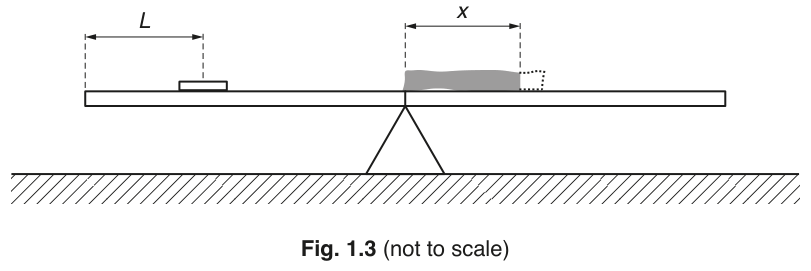
• Measure and record the new values of $x$ and $L$ .

$x$ = ______ $\text{cm}$
$L$ = ______ $\text{cm}$

DifficultyMedium-Easy

Worked solution

Reduce $x$ by cutting off about $1\ \text{cm}$ of clay (furthest from the line), rebalance by moving the mass, then measure $x$ and $L$ .

Example readings (to nearest $0.1\ \text{cm}$ ):

x = 19.0\ \text{cm}

L = 12.2\ \text{cm}

Final answer

x = 19.0 cm, L = 12.2 cm (example)

Detailed explanation

Background Concept

To obtain a relationship between variables experimentally, you vary one quantity systematically and measure the corresponding change in another. Here, the modelling clay length $x$ is reduced step-by-step, and for each $x$ you adjust the mass position until the strip is balanced, then measure $L$ .

Understanding the Question

You must:

shorten the modelling clay by about $1\ \text{cm}$ (cut from the end furthest from the marked line),
rebalance the strip by moving the mass,
then record the new $x$ and $L$ .

Approach

Shorten the clay slightly (so $x$ changes in a controlled way).
Achieve balance again (so each reading corresponds to equilibrium).
Measure $x$ and $L$ with the same ruler and same precision as before.

Step-by-Step Reasoning

Remove approximately $1\ \text{cm}$ from the far end of the clay so the end above the line remains in the same reference position.
Place the clay back on the strip with one end above the line.
Slide the mass until the strip just balances (no tendency to rotate).
Measure $x$ (length of clay) and $L$ (distance from centre of mass to end of strip).
Record both to $0.1\ \text{cm}$ .

Key Takeaways

Change only the intended variable ( $x$ ), then re-establish balance before measuring.
Record paired $(x, L)$ data with consistent precision.

Common Mistakes

Cutting from the wrong end (which changes the reference point for $x$ ).
Measuring before rebalancing.
Not keeping the clay as a uniform cylinder (can make positioning ambiguous).

Things to Be Careful About

Ensure the prism position and the marked line are used consistently.
When the strip is nearly balanced, small movements matter; adjust gently and wait for it to settle.

Techniques used

change the independent variable by a controlled small amountrebalance the system to regain equilibriummeasure and record paired values with consistent precision

(c)

Continue to reduce $x$ until you have six sets of values of $x$ and $L$ . You may include your previous results.

Record your results in a table. Include values of $x^2$ in the table.

DifficultyMedium

Worked solution

Record at least six sets of $x$ and $L$ and calculate $x^2$ for each.

Example table (all lengths to nearest $0.1\ \text{cm}$ ):

$x$ / $\text{cm}$	$L$ / $\text{cm}$	$x^2$ / $\text{cm}^2$
$20.0$	$13.0$	$400.0$
$19.0$	$12.2$	$361.0$
$18.0$	$11.5$	$324.0$
$17.0$	$10.8$	$289.0$
$16.0$	$10.1$	$256.0$
$15.0$	$9.5$	$225.0$

Final answer

Table of six (x, L) values with calculated x^2 (example shown)

Detailed explanation

Background Concept

In Paper 3, marks for tables are awarded for how you record and present data as much as for the numbers themselves. A good results table must:

include all readings in one clear table,
have headings that include quantity and unit (e.g. $x / \text{cm}$ ),
show consistent precision within each column,
include any calculated columns requested (here $x^2$ ).

Calculated quantities should be consistent with the precision of the measured quantities (you cannot justify an extra level of precision beyond your raw data).

Understanding the Question

You must continue reducing $x$ and rebalancing until you have six sets of $(x, L)$ . You may include earlier values from parts (a) and (b). You must then produce a table that includes $x$ , $L$ , and $x^2$ .

Approach

Choose a sensible range of $x$ values by reducing the clay in roughly equal steps (about $1\ \text{cm}$ each time).
For each $x$ , rebalance the strip and then measure $L$ .
Create a single table with three columns: $x$ , $L$ , and $x^2$ .
Compute $x^2$ for each row using $x^2 = x \times x$ .

Step-by-Step Reasoning

Start from your initial $x$ (about $20\ \text{cm}$ ) and reduce it systematically.
For each new $x$ , slide the mass until the strip balances.
Measure $x$ and $L$ with the same method each time.
Set up your table with headings including units:
- $x / \text{cm}$
- $L / \text{cm}$
- $x^2 / \text{cm}^2$
Fill in the measured values to the nearest $0.1\ \text{cm}$ .
Calculate $x^2$ . For example, if $x = 19.0\ \text{cm}$ , then:

x^2 = (19.0)^2 = 361.0\ \text{cm}^2

Keep decimal places consistent in each column (e.g. all $x$ values to 1 d.p., all $L$ values to 1 d.p.).

Key Takeaways

A clear table with correct headings, units, and consistent precision is essential.
Always include the requested derived quantity ( $x^2$ ) and its unit.

Common Mistakes

Missing units in the headings.
Splitting results across multiple tables.
Using inconsistent decimal places within a column.
Forgetting to include the $x^2$ column, or calculating $x^2$ incorrectly.

Things to Be Careful About

If you record $x$ to $0.1\ \text{cm}$ , do not record $L$ to $0.01\ \text{cm}$ unless your instrument supports that.
Ensure you have a good spread of $x$ values (not all very close together), because this improves the graph and the gradient accuracy.

Techniques used

collect at least six paired measurements over a suitable rangecalculate derived quantities for each rowrecord results in a single table with headings and unitsuse consistent decimal places within each column

(d)

(i)

Plot a graph of $L$ on the $y$ -axis against $x^2$ on the $x$ -axis.

DifficultyMedium

Worked solution

Plot a graph of $L$ (y-axis) against $x^2$ (x-axis):

x-axis label: $x^2 / \text{cm}^2$
y-axis label: $L / \text{cm}$
use a convenient scale occupying at least half the grid on each axis
plot all six points accurately.

Final answer

Graph plotted: L vs x^2 (axes labelled with units, points plotted)

Detailed explanation

Background Concept

A graph is used to test whether two quantities are related, and to extract constants from the relationship. For full graph marks you must:

label axes with quantity and unit,
use sensible scales (not cramped; not awkward like 3 squares = 1 unit),
plot points accurately with small, neat crosses,
use all your data points.

Understanding the Question

You must plot $L$ on the y-axis against $x^2$ on the x-axis using your table values from part (c).

Approach

Decide which quantity goes on each axis (given in the question).
Choose scales that use at least half the graph paper in both directions.
Label both axes correctly.
Plot each point $(x^2, L)$ .

Step-by-Step Reasoning

Take your $x^2$ values as x-coordinates and your $L$ values as y-coordinates.
Choose a scale such that the smallest and largest $x^2$ values fit comfortably (e.g. if $x^2$ ranges from about $225$ to $400\ \text{cm}^2$ , you might use 2 cm per 20 or 25 $\text{cm}^2$ ).
Similarly choose a y-scale so that the $L$ range fits well.
Label axes as $x^2 / \text{cm}^2$ and $L / \text{cm}$ .
Plot each point with a small cross; accuracy is judged by placement relative to grid intersections.

Key Takeaways

Axis labels must include units.
Good scaling and accurate plotting are essential for reliable gradient/intercept.

Common Mistakes

Swapping axes (plotting $x^2$ on y-axis).
Missing units or writing only the unit without the quantity.
Using a very small part of the graph paper.

Things to Be Careful About

Do not join the dots point-to-point; you will draw a best-fit line in (ii).
Plot using the correct pairings from the same row of the table (do not mix rows).

Techniques used

choose suitable axis scales that use at least half the gridlabel axes with quantity and unitplot points accurately from a results table

(ii)

Draw the straight line of best fit.

DifficultyMedium-Easy

Worked solution

Draw a single straight line of best fit through the plotted points, with roughly equal scatter of points about the line.

Final answer

Straight best-fit line drawn

Detailed explanation

Background Concept

A best-fit line represents the overall trend of data when a linear relationship is expected. It should not be forced through every point; instead it should pass through the region where the points cluster, leaving a similar number of points above and below the line.

Understanding the Question

After plotting $L$ against $x^2$ , you must draw the straight line of best fit.

Approach

Use a ruler to draw one straight line.
Position it so the scatter is balanced.

Step-by-Step Reasoning

Look at the general trend of the points.
Place a ruler so that the line passes centrally through the set of points.
Ensure the line extends across the full range of your data (not a short segment only).

Key Takeaways

A best-fit line is about trend, not connecting points.

Common Mistakes

Joining points dot-to-dot.
Drawing a line that favours one outlier point, leaving most points on one side.

Things to Be Careful About

Use a sharp pencil and a ruler.
Do not draw multiple lines; only one best-fit line should be shown.

Techniques used

judge the overall trend of the plotted pointsdraw a straight line of best fit with balanced scatter

(iii)

Determine the gradient and $y$ -intercept of this line.

gradient = ______
$y$ -intercept = ______

DifficultyMedium

Worked solution

Working

Using two well-separated points on the best-fit line, e.g.

(x^2, L) = (400\ \text{cm}^2,\ 13.0\ \text{cm})\ \text{and}\ (225\ \text{cm}^2,\ 9.5\ \text{cm})

\text{gradient} = \frac{\Delta L}{\Delta (x^2)} = \frac{13.0 - 9.5}{400 - 225} = \frac{3.5}{175} = 2.0 \times 10^{-2}\ \text{cm}^{-1}

y\text{-intercept} = 5.0\ \text{cm}

Answer

gradient $= 2.0 \times 10^{-2}\ \text{cm}^{-1}$

y-intercept $= 5.0\ \text{cm}$

Final answer

gradient = 2.0 × 10^-2 cm^-1, y-intercept = 5.0 cm (example)

Detailed explanation

Background Concept

For a straight-line graph, the gradient (slope) is defined by:

\text{gradient} = \frac{\Delta y}{\Delta x}

and the y-intercept is the value of $y$ when $x = 0$ .

In this experiment you plot $L$ on the y-axis against $x^2$ on the x-axis, so:

$y \equiv L$ (unit cm)
$x \equiv x^2$ (unit $\text{cm}^2$ )

Therefore the gradient unit is:

\frac{\text{cm}}{\text{cm}^2} = \text{cm}^{-1}

Understanding the Question

You must obtain numerical values for:

the gradient of your best-fit line on the $L$ vs $x^2$ graph,
the y-intercept of that line.

These should come from the drawn best-fit line (not from joining individual points).

Approach

Pick two points on the best-fit line that are far apart to form a large triangle.
Calculate the gradient using $\Delta L / \Delta(x^2)$ .
Extend the best-fit line to cross the y-axis and read the intercept.

Step-by-Step Reasoning

Choose two points on the line that are easy to read (often where the line crosses grid intersections).
Compute changes:
- $\Delta L$ is the vertical change in cm.
- $\Delta(x^2)$ is the horizontal change in $\text{cm}^2$ .
Divide to obtain the gradient, and include units $\text{cm}^{-1}$ .
For the y-intercept, set $x^2 = 0$ (the y-axis) and read the value of $L$ where your best-fit line crosses the y-axis; include unit cm.

Key Takeaways

Always use the best-fit line for gradient and intercept.
Use a large triangle to reduce percentage reading uncertainty.
Include correct units: gradient in $\text{cm}^{-1}$ and intercept in cm.

Common Mistakes

Using two data points not on the best-fit line (especially if they are outliers).
Using $\Delta x / \Delta y$ instead of $\Delta y / \Delta x$ .
Forgetting units, or giving gradient in cm (wrong).

Things to Be Careful About

Read coordinates from the line accurately; choose points far apart.
The y-intercept may require extending the line back to $x^2 = 0$ ; use a ruler and do not guess.

Techniques used

use a large triangle to determine gradientcalculate gradient as \Delta y / \Delta x with unitsread the y-intercept from the best-fit line

(e)

It is suggested that the quantities $L$ and $x$ are related by the equation

L = ax^2 + b

where $a$ and $b$ are constants.

Use your answers in (d)(iii) to determine the values of $a$ and $b$ .
Give appropriate units.

$a$ = ______
$b$ = ______

DifficultyMedium-Easy

Worked solution

Since

L = ax^2 + b

and the graph is $L$ (y) against $x^2$ (x),

a = \text{gradient}, \qquad b = y\text{-intercept}

Using (d)(iii):

a = 2.0 \times 10^{-2}\ \text{cm}^{-1}

b = 5.0\ \text{cm}

Final answer

a = 2.0 × 10^-2 cm^-1, b = 5.0 cm (example)

Detailed explanation

Background Concept

A linear equation has the form:

y = mx + c

where $m$ is the gradient and $c$ is the y-intercept.

Here you are given:

L = ax^2 + b

If you plot $L$ on the y-axis against $x^2$ on the x-axis, the equation is already linear in the plotted variables:

y-variable: $L$
x-variable: $x^2$

So it matches $y = mx + c$ directly, with $a$ playing the role of the gradient and $b$ the role of the intercept.

Units:

$L$ has unit cm.
$x^2$ has unit $\text{cm}^2$ .
So

[a] = \frac{\text{cm}}{\text{cm}^2} = \text{cm}^{-1}

and

[b] = \text{cm}

Understanding the Question

You must use your measured gradient and y-intercept from (d)(iii) to state the constants $a$ and $b$ , including appropriate units.

Approach

Identify $a$ as the gradient of the $L$ vs $x^2$ graph.
Identify $b$ as the y-intercept of that graph.
Attach the correct units based on the axes.

Step-by-Step Reasoning

From the plotted relationship $L = ax^2 + b$ and the graph of $L$ (y) against $x^2$ (x):

a = \text{gradient}

b = y\text{-intercept}

If your gradient is, for example, $2.0 \times 10^{-2}$ and $L$ is in cm while $x^2$ is in $\text{cm}^2$ , then:

a = 2.0 \times 10^{-2}\ \text{cm}^{-1}

If your y-intercept is, for example, $5.0$ , then:

b = 5.0\ \text{cm}

Key Takeaways

When the plotted variables match the equation form, constants are read directly as gradient and intercept.
Units come from the ratio of y-units to x-units for the gradient.

Common Mistakes

Giving $a$ the wrong unit (e.g. cm or $\text{cm}^2$ ).
Swapping $a$ and $b$ .
Using values from a single data pair rather than the best-fit line values.

Things to Be Careful About

Ensure you used the correct graph orientation: $L$ vs $x^2$ .
Quote $a$ and $b$ to a sensible number of significant figures consistent with your graph readings.

Techniques used

match an experimental straight-line graph to y = mx + cidentify constants from gradient and interceptassign correct units to derived constants

The rest of this paper

1 more questions

Q2Manipulation, Measurement and Observation · Analysis, Conclusions and Evaluation · Presentation of Data and Observations1M

Loading the full paper…