Physics 9702/34 — May/June 2019

Cambridge AS Level · Advanced Practical Skills · worked solutions for every part, with the mark scheme

questions

marks

120

minutes

Topics Manipulation, Measurement and Observation · Presentation of Data and Observations · Analysis, Conclusions and Evaluation

Q1Manipulation, Measurement and ObservationPresentation of Data and ObservationsAnalysis, Conclusions and EvaluationFree sample

In this experiment, you will investigate the equilibrium position of a cardboard triangle.

(a)

• Assemble the apparatus as shown in Fig. 1.1, with the nail passing through the hole marked A and the wire hook passing through one of the remaining holes.

• Ensure that the nail is held securely in the clamp and that the cardboard triangle can swing freely on the nail.

Fig. 1.1

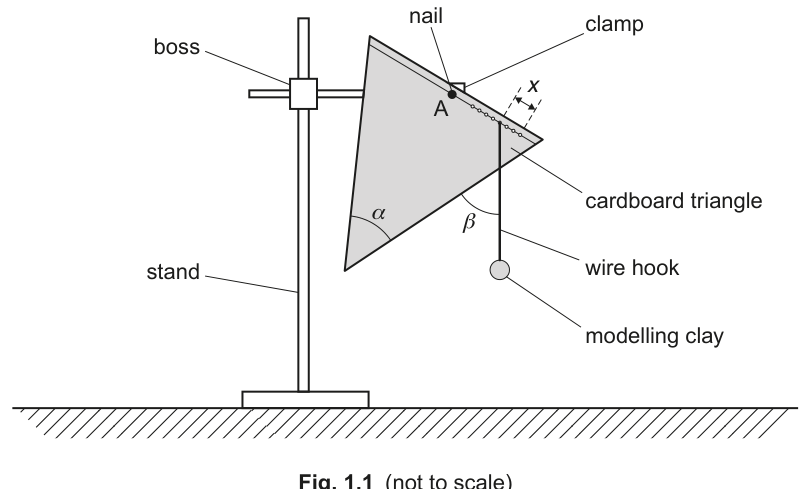
• The angle of the lower corner of the card is $\alpha$ , as shown in Fig. 1.1.

• Measure and record $\alpha$ .

$\alpha$ = ______ $^{\circ}$

• Calculate the value of $\frac{\alpha}{2}$ .

$\frac{\alpha}{2}$ = ______ $^{\circ}$

DifficultyEasy

Worked solution

Working

Measure $\alpha$ using a protractor (to the nearest $1^\circ$ ).

Example:

\alpha = 60^\circ

\frac{\alpha}{2} = \frac{60^\circ}{2} = 30^\circ

Answer

$\alpha = 60^\circ$ (example)

$\dfrac{\alpha}{2} = 30^\circ$

Final answer

α = 60°, α/2 = 30° (example)

Detailed explanation

Background Concept

Angles in this practical are measured directly with a protractor. Any later calculations (such as (\alpha/2)) inherit the precision of the original measurement.

Understanding the Question

You are told that the cardboard triangle has a lower-corner angle (\alpha) (shown on Fig. 1.1). You must:

measure (\alpha) and record it with units of degrees,
calculate (\alpha/2).

Approach

Use a protractor to measure (\alpha) from the diagram on the apparatus.
Record (\alpha) to a sensible precision (typically nearest (1^\circ)).
Divide by 2 to obtain (\alpha/2), keeping the same degree unit.

Step-by-Step Reasoning

Place the centre of the protractor at the vertex of the lower corner of the triangle.
Align the zero line with one edge of the triangle and read the angle to the other edge.
Suppose the measured value is (\alpha = 60^\circ) (this is an example only; your value depends on your card).
Then

\frac{\alpha}{2} = \frac{60^\circ}{2} = 30^\circ.

Key Takeaways

Record angle measurements with units (degrees).
Derived quantities should be calculated clearly and sensibly rounded.

Common Mistakes

Omitting the unit (^{\circ}).
Recording (\alpha) with unrealistic precision (e.g. (60.0^\circ) with a basic protractor).
Making an arithmetic slip when halving (\alpha).

Things to Be Careful About

Parallax when reading the protractor scale.
Using the correct protractor scale (inner vs outer markings).
If the protractor cannot be positioned accurately on the card, estimate carefully and be consistent with precision.

Techniques used

measure an angle with a protractorrecord a reading to an appropriate precision with unitcalculate a derived quantity from a measured value

(b)

• The angle between the wire hook and the edge of the card is $\beta$ , as shown in Fig. 1.1.

Measure and record $\beta$ .

$\beta$ = ______ $^{\circ}$

• The distance between the hole with the wire hook in it and the hole furthest from A is $x$ , as shown in Fig. 1.1.

Measure and record $x$ .

$x$ = ______ $\text{cm}$

DifficultyEasy

Worked solution

Working

Measure $\beta$ using a protractor (nearest $1^\circ$ ) and measure $x$ using a ruler (nearest $1\ \text{mm}$ or $0.1\ \text{cm}$ ).

Example:

\beta = 53^\circ

x = 8.0\ \text{cm}

Answer

$\beta = 53^\circ$ (example)

$x = 8.0\ \text{cm}$

Final answer

β = 53°, x = 8.0 cm (example)

Detailed explanation

Background Concept

In Paper 3, credit is given for taking careful measurements and recording them with sensible precision and correct units. Angles are typically read to the nearest degree and lengths with a ruler to the nearest millimetre.

Understanding the Question

From Fig. 1.1:

(\beta) is the angle between the wire hook (vertical line) and the edge of the card.
(x) is the distance between the hole containing the hook and the hole furthest from A.
You must measure and record both values.

Approach

Use a protractor for (\beta) and a ruler for (x).
Record each measurement with its unit: degrees for (\beta), cm for (x).

Step-by-Step Reasoning

For (\beta): place the protractor so that one reference line lies along the card edge and read the angle to the wire hook direction (the hook is vertical). Read to nearest (1^\circ).
For (x): use a ruler to measure the straight-line distance between the centres of the two specified holes. Read to nearest (0.1\ \text{cm}) (or better if your ruler allows).
A representative example set might be (\beta = 53^\circ) and (x = 8.0\ \text{cm}) (your own readings will differ).

Key Takeaways

Match instrument to quantity: protractor for angles, ruler for lengths.
Record units and sensible precision.

Common Mistakes

Measuring (x) between the outer edges of holes rather than between centres.
Forgetting that (\beta) is between the hook (vertical) and the edge of the card (not between two card edges).
Writing (x) with no unit or in mm when the answer line requests cm.

Things to Be Careful About

Ensure the triangle swings freely so the hook truly hangs vertically (otherwise (\beta) is not well-defined).
Avoid parallax when reading the protractor and ruler.
Keep the same precision for all repeated measurements later (use consistent decimal places for (x)).

Techniques used

measure an angle with a protractormeasure a length with a rulerrecord readings to appropriate precision with units

(c)

Move the wire hook to another hole and repeat (b) until you have six sets of values of $\beta$ and $x$ .

Record your results in a table.
Include values of $\tan\left(\beta - \frac{\alpha}{2}\right)$ in your table.

10M

DifficultyMedium

Worked solution

Answer

Take six different positions of the hook (six different holes) and for each position measure $x$ and $\beta$ .

Record all results in one table with clear headings and units, including a calculated column for $\tan\left(\beta-\frac{\alpha}{2}\right)$ .

Example layout (values shown are illustrative only):

set	$x/\text{cm}$	$\beta/^{\circ}$	$\left(\beta-\frac{\alpha}{2}\right)/^{\circ}$	$\tan\left(\beta-\frac{\alpha}{2}\right)$
1	2.0	41.3	11.3	0.20
2	4.0	46.7	16.7	0.30
3	6.0	50.5	20.5	0.40
4	8.0	53.4	23.4	0.50
5	10.0	55.6	25.6	0.60
6	12.0	57.0	27.0	0.70

Final answer

Single table of 6 readings of x and β with calculated tan(β − α/2)

Detailed explanation

Background Concept

A good practical table:

contains all readings in one clear table,
has column headings with quantity and unit (e.g. (x/\text{cm}), (\beta/^{\circ})),
uses consistent decimal places within a column,
includes any required calculated quantities.

Here you must calculate

y = \tan\left(\beta - \frac{\alpha}{2}\right)

for each pair of (\beta) and (x), where (\alpha) is the single angle you measured earlier.

Understanding the Question

You must:

move the hook to different holes so that (x) changes,
for each position measure (x) and (\beta),
obtain 6 sets of ((x,\beta)),
present them in a table including the derived quantity (\tan\left(\beta-\alpha/2\right)).

Approach

Decide that (x) is the variable you change (by moving the hook), and (\beta) is measured for each value.
Choose holes that give a good spread of (x) values (not all clustered together).
Make a results table with headings and units.
For each row, compute (\beta - \alpha/2) and then take the tangent using a calculator in degree mode.

Step-by-Step Reasoning

Start with your measured (\alpha) and compute (\alpha/2) once.
For each hook position:
- measure (x) (e.g. to (0.1\ \text{cm})),
- measure (\beta) (to nearest (1^\circ)),
- calculate (\theta = \beta - \alpha/2) (in degrees),
- calculate (\tan \theta) and record it to a sensible number of significant figures (often 2 or 3 is fine).

A typical table structure is:

a column for (x),
a column for (\beta),
optionally a column for (\beta-\alpha/2) (often helpful to show your working),
a column for (\tan(\beta-\alpha/2)).

Key Takeaways

Good data needs both quantity (6 readings) and range (spread of (x)).
Calculated columns must be clearly identified and based on measured values.
Consistent formatting (units, decimal places) earns marks in practical papers.

Common Mistakes

Fewer than six sets of readings.
Missing units in headings (e.g. writing just (x) instead of (x/\text{cm})).
Calculating (\tan(\beta) - \alpha/2) instead of (\tan(\beta-\alpha/2)).
Calculator in radians mode, giving incorrect tangent values.

Things to Be Careful About

Ensure (\beta) and (\alpha/2) are both in degrees before subtraction.
Use consistent precision: do not mix (8\ \text{cm}) and (8.00\ \text{cm}) in the same column unless justified.
Choose (x) values that will produce a clear trend for the later graph (avoid repeated or nearly identical (x) values).

Techniques used

take a suitable range of readings by changing the independent variablerecord results in a single table with headings and unitscalculate a derived column using a trigonometric functionuse consistent significant figures within each column

(d)

(i)

Plot a graph of $\tan\left(\beta - \frac{\alpha}{2}\right)$ on the $y$ -axis against $x$ on the $x$ -axis.

DifficultyMedium-Easy

Worked solution

Answer

Plot a graph with:

$y$ -axis: $\tan\left(\beta-\frac{\alpha}{2}\right)$ (no unit)
$x$ -axis: $x / \text{cm}$

Use a suitable scale (at least half the grid on each axis) and plot all six points accurately.

Final answer

Graph of tan(β − α/2) (y) against x / cm (x)

Detailed explanation

Background Concept

A good graph in Paper 3 requires:

correct choice of variables on axes,
clear axis labels (quantity and unit),
sensible scales (not cramped; not awkward increments),
accurate plotting of all points.

Understanding the Question

You have calculated values of

y = \tan\left(\beta-\frac{\alpha}{2}\right)

for each measured (x). You must plot (y) (vertical axis) against (x) (horizontal axis).

Approach

Put the independent variable (x) on the horizontal axis.
Put the dependent/derived variable (\tan(\beta-\alpha/2)) on the vertical axis.
Choose scales so your points spread across the page.

Step-by-Step Reasoning

Draw axes and label them:
- horizontal: (x/\text{cm}),
- vertical: (\tan(\beta-\alpha/2)) (dimensionless).
Choose a scale such that the smallest and largest values from your table fit comfortably and use at least half of the available grid.
Plot each point ((x,y)) carefully using a sharp pencil; marks should be small crosses.
Check each point is in the correct place by re-reading the table before moving on.

Key Takeaways

Axes must be labelled with both quantity and unit (unit omitted only if none).
A good scale makes the best-fit line and gradient determination more accurate.

Common Mistakes

Swapping axes (plotting (x) on the (y)-axis).
Writing an axis label without the unit for (x).
Using a scale like 3 squares = 1 unit (awkward) which makes reading values difficult.

Things to Be Careful About

(\tan(\beta-\alpha/2)) has no unit; do not invent one.
Do not force the graph to start at the origin unless your data naturally requires it; choose a scale based on your measured range.

Techniques used

choose suitable axes and scales to use most of the graph gridlabel axes with quantity and unitplot points accurately from a results table

(ii)

Draw the straight line of best fit.

DifficultyEasy

Worked solution

Answer

Draw one straight line of best fit through the plotted points (balanced with roughly equal scatter above and below the line).

Final answer

Straight line of best fit drawn

Detailed explanation

Background Concept

A best-fit line represents the overall linear trend of the data. In practical work, points rarely lie perfectly on a straight line because of random uncertainties.

Understanding the Question

After plotting (\tan(\beta-\alpha/2)) against (x), you must draw the straight line of best fit.

Approach

Use a ruler.
Aim for a line that reflects the trend and is not forced through every point.

Step-by-Step Reasoning

Visually judge the overall trend of the plotted points.
Place a ruler so that the line passes through the middle of the cluster.
Ensure there are approximately equal numbers of points on each side of the line (or that the distances of points above and below are balanced).
Draw a single straight line, extended well across the graph to make gradient determination easier.

Key Takeaways

The best-fit line is about the trend, not about connecting points.
Extending the line helps reduce fractional error when reading gradient.

Common Mistakes

Joining the points dot-to-dot.
Forcing the line through the origin when the intercept is not zero.
Drawing a line that goes through an outlier at the expense of the rest of the points.

Things to Be Careful About

Use a sharp pencil and a thin line; thick lines reduce reading accuracy.
Do not change the line later to make calculations ‘nice’; it must reflect the plotted data.

Techniques used

draw a single straight line of best fit through scattered pointsbalance points above and below the best-fit line

(iii)

Determine the gradient and $y$ -intercept of this line.

gradient = ______
$y$ -intercept = ______

DifficultyMedium

Worked solution

Working

Use a large triangle on the best-fit line.

Example using two well-separated points on the line (illustrative):

(x_1,y_1)=(2.0,0.20),\quad (x_2,y_2)=(12.0,0.70)

\text{gradient} = \frac{\Delta y}{\Delta x} = \frac{0.70-0.20}{12.0-2.0} = \frac{0.50}{10.0} = 0.050\ \text{cm}^{-1}

$y$ -intercept read at $x=0$ (illustrative):

\text{intercept} = 0.10

Answer

gradient $= 0.050\ \text{cm}^{-1}$ (example)

$y$ -intercept $= 0.10$ (example)

Final answer

gradient = 0.050 cm^-1, y-intercept = 0.10 (example)

Detailed explanation

Background Concept

For a straight-line graph of (y) against (x):

y = mx + c

(m) is the gradient (slope): (m = \Delta y / \Delta x).
(c) is the y-intercept: the value of (y) when (x=0).

Graph-reading uncertainty is reduced by using points far apart on the best-fit line.

Understanding the Question

You have drawn a straight line on a plot of (y = \tan(\beta-\alpha/2)) against (x). You must find:

the gradient of the best-fit line,
the y-intercept.

Approach

Choose two points on the best-fit line that are far apart (not necessarily original data points).
Read their coordinates accurately.
Compute (m = (y_2-y_1)/(x_2-x_1)).
Read off the intercept at (x=0) by extending the line to the y-axis.

Step-by-Step Reasoning

Draw a large gradient triangle on the best-fit line to maximise (\Delta x) and (\Delta y), making percentage reading errors smaller.
Suppose (as an illustration) the best-fit line passes near ((2.0, 0.20)) and ((12.0, 0.70)).
Then:

\Delta y = 0.70 - 0.20 = 0.50

\Delta x = 12.0 - 2.0 = 10.0\ \text{cm}

and

\text{gradient} = \frac{\Delta y}{\Delta x} = \frac{0.50}{10.0\ \text{cm}} = 0.050\ \text{cm}^{-1}.

The y-intercept is where the line crosses the y-axis ((x=0)). Read this value directly; in the illustrative example it is (0.10).

Units:

(y) is dimensionless.
(x) is in (\text{cm}).
So gradient has units (\text{cm}^{-1}), and the intercept is dimensionless.

Key Takeaways

Gradient is always (\Delta y/\Delta x) using the axes variables.
Use a large triangle and points on the best-fit line.
Intercept is a reading at (x=0), not at the first data point.

Common Mistakes

Calculating (\Delta x/\Delta y) instead of (\Delta y/\Delta x).
Using two adjacent points, giving a large percentage uncertainty.
Forgetting units for the gradient.
Taking the intercept from an extrapolation that does not reach (x=0) (line not extended far enough).

Things to Be Careful About

Read coordinates to the precision allowed by the graph scale.
Use points on the best-fit line, not the raw scattered points.
If (x) axis is labelled in cm, your gradient must be in (\text{cm}^{-1}) (not (\text{m}^{-1}) unless you converted (x) to metres).

Techniques used

determine gradient from a large triangle on the best-fit lineread y-intercept from the graph at x = 0use correct units for gradient from axis units

(e)

It is suggested that the quantities $\beta$ , $\alpha$ and $x$ are related by the equation

\tan\left(\beta - \frac{\alpha}{2}\right) = Px + Q

where $P$ and $Q$ are constants.

Use your answers in (d)(iii) to determine the values of $P$ and $Q$ .
Give appropriate units.

$P$ = ______
$Q$ = ______

DifficultyMedium-Easy

Worked solution

Working

Given

\tan\left(\beta-\frac{\alpha}{2}\right)=Px+Q

This is of the form $y=mx+c$ for the graph of $y=\tan\left(\beta-\frac{\alpha}{2}\right)$ against $x$ .

P=\text{gradient},\quad Q=\text{y-intercept}.

Using the values from (d)(iii) (example):

P = 0.050\ \text{cm}^{-1}

Q = 0.10

Answer

$P = 0.050\ \text{cm}^{-1}$ (example)

$Q = 0.10$ (dimensionless, example)

Final answer

P = gradient (cm^-1), Q = y-intercept (dimensionless)

Detailed explanation

Background Concept

If a relationship can be written as

y = Px + Q,

then plotting (y) against (x) gives a straight line with:

gradient (=P),
y-intercept (=Q).

Units follow from the axes:

(y) here is a tangent, so it is dimensionless.
(x) is a length measured in cm.
So (P) must have units of (\text{cm}^{-1}) and (Q) has no units.

Understanding the Question

You are told that:

\tan\left(\beta-\frac{\alpha}{2}\right)=Px+Q.

You have already obtained the gradient and y-intercept from your graph in (d)(iii). You must use them to state numerical values for (P) and (Q), with appropriate units.

Approach

Recognise the correspondence between the suggested equation and (y=mx+c).
Set (P) equal to the gradient and (Q) equal to the intercept.
Assign units using axis units.

Step-by-Step Reasoning

Let

y = \tan\left(\beta-\frac{\alpha}{2}\right).

Then the suggested equation becomes

y = Px + Q.

Your graph is exactly (y) against (x), so it is already linear. Therefore:

the gradient you measured in (d)(iii) is (P),
the intercept you measured is (Q).

If (illustratively) your gradient was (0.050\ \text{cm}^{-1}) and intercept was (0.10), then:

P = 0.050\ \text{cm}^{-1},\qquad Q = 0.10.

Key Takeaways

Comparing with (y=mx+c) is the standard way to extract constants from a straight-line graph.
Always use axis units to determine the unit of a gradient-based constant.

Common Mistakes

Swapping (P) and (Q).
Giving (Q) a unit (it should be dimensionless here).
Using the gradient from a line drawn between two data points instead of the best-fit line.

Things to Be Careful About

If you used (x) in cm on the graph, then (P) is in (\text{cm}^{-1}). If you converted (x) to m, then (P) would be in (\text{m}^{-1}). Your stated unit must match what you plotted.
Quote (P) and (Q) to a sensible number of significant figures consistent with graph-reading precision.

Techniques used

match an experimental graph to a linear equationidentify constants from gradient and interceptdeduce units of constants from axis units

The rest of this paper

1 more questions

Q2Manipulation, Measurement and Observation · Analysis, Conclusions and Evaluation · Presentation of Data and Observations20M

Loading the full paper…