Physics 9702/31 — May/June 2019

Cambridge AS Level · Advanced Practical Skills · worked solutions for every part, with the mark scheme

questions

marks

120

minutes

Topics Manipulation, Measurement and Observation · Presentation of Data and Observations · Analysis, Conclusions and Evaluation

Q1Manipulation, Measurement and ObservationPresentation of Data and ObservationsAnalysis, Conclusions and EvaluationFree sample

In this experiment, you will investigate the forces acting on a metre rule.

(a) • Set up the apparatus as shown in Fig. 1.1.

Fig. 1.1

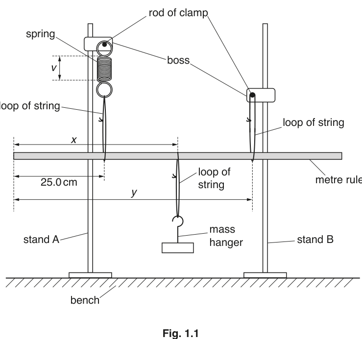
• The distance between the end of the rule and the loop of string attached to the spring is $25.0\text{ cm}$ . Keep this distance constant throughout the experiment.

The distance between the end of the rule and the loop of string supporting the mass hanger is $x$ .

The distance between the end of the rule and the loop of string attached to stand B is $y$ .

Adjust the apparatus until $x = 50.0\text{ cm}$ and $y = 75.0\text{ cm}$ .

• The strings and spring should be vertical and the rule should be parallel to the bench.

The length of the coiled section of the spring is $v$ . To view this more clearly, you may use the adhesive putty to attach the white card to stand A behind the spring.

Measure and record $v$ .

(a)

$v$ = ______

DifficultyEasy

Worked solution

Measure the length of the coiled section of the spring $v$ using a ruler (eye level).

Example reading:

v = 4.80\ \text{cm}

Final answer

v ≈ 4.80 cm (example)

Detailed explanation

Background Concept

In Paper 3 practical work, marks for a “measure and record” step are awarded for (i) taking the correct measurement of the stated quantity, and (ii) recording it with sensible precision and a unit.

A spring’s “coiled section length” $v$ is a length measurement, so it should be read from a scale with the eye perpendicular to the scale to reduce parallax error.

Understanding the Question

You are told that the apparatus must be adjusted so that the metre rule is parallel to the bench (horizontal) and the spring and strings are vertical. You then measure $v$ , the length of the coiled part of the spring.

So the task is simply: set the geometry correctly, then read and record $v$ .

Approach

Ensure the rule is horizontal and the spring is vertical (so $v$ is a true vertical length).
Read $v$ from the scale (or against the white card) at eye level.
Record $v$ with an appropriate unit and precision.

Step-by-Step Reasoning

With the rule level and the spring vertical, the coiled section has a well-defined length.
Place your eye in line with the endpoints of the coiled section (not above or below).
Read off the length using a ruler/metre rule; record to the nearest mm ( $0.1\ \text{cm}$ ) if that is the smallest clear scale division.
Write the value with unit, e.g. $v = 4.80\ \text{cm}$ .

Key Takeaways

Practical marks often depend on how you measure and how you record (unit + appropriate precision).
Keeping the spring vertical reduces systematic error in measuring a vertical length.

Common Mistakes

Omitting the unit.
Recording an unrealistic precision (e.g. too many decimal places for a simple ruler reading).
Measuring the wrong part of the spring (including hooks/uncoiled sections).

Things to Be Careful About

Parallax: read at eye level.
Identify the exact endpoints of the “coiled section”.
Keep the rule horizontal; if the spring is tilted, the measured length is not the true vertical length.

Techniques used

align the apparatus so the rule is horizontal and strings are verticalread a length from a scale at eye level to avoid parallaxrecord a measurement to an appropriate precision with unit

(b)

• Change $x$ by moving the loop of string supporting the mass hanger to a different position on the rule.

• Move stand B and slide the loop of string attached to stand B along the rule until $v$ has the same value as in (a).

• Ensure the strings and spring are vertical and the rule should be parallel to the bench.

• Measure and record $x$ and $y$ .

$x$ = ______
$y$ = ______

DifficultyMedium-Easy

Worked solution

Move the mass hanger loop to a new position to change $x$ . Adjust stand B / the loop position until $v$ is the same as in (a). Measure $x$ and $y$ .

Example set:

x = 45.0\ \text{cm}

y = 70.5\ \text{cm}

Final answer

x ≈ 45.0 cm, y ≈ 70.5 cm (example)

Detailed explanation

Background Concept

In this experiment you are changing one position ( $x$ ) and then adjusting another position ( $y$ ) until the spring length $v$ returns to the same value. This “keep $v$ constant” instruction is important because it keeps the spring extension (and therefore the spring force) constant.

For practical marks, what matters is that you can:

change the loop position reliably,
re-adjust to meet the condition ( $v$ same as before),
measure and record $x$ and $y$ correctly.

Understanding the Question

You must:

change $x$ by moving the mass hanger loop,
move stand B and slide the loop on the rule until $v$ matches the value from (a),
then measure and record the new $x$ and $y$ .

Approach

Treat $x$ as the value you choose (by placing the mass hanger loop).
Treat $y$ as the value you must adjust until the spring returns to the same extension (same $v$ ).
Once balanced (rule horizontal, strings vertical, correct $v$ ), read $x$ and $y$ along the rule.

Step-by-Step Reasoning

Move the mass hanger loop to a clearly different mark (large change helps produce a good range of data).
Slide/move stand B and the loop attached to stand B until the coil length $v$ is the same as in (a).
Check alignment: rule horizontal, strings and spring vertical.
Read $x$ as the distance from the end of the rule (as defined in the stem) to the mass hanger loop.
Read $y$ similarly to the support loop at stand B.
Record both in $\text{cm}$ to the same precision each time (commonly $0.1\ \text{cm}$ ).

Key Takeaways

Achieving the condition (same $v$ ) comes before recording $x$ and $y$ .
Large spread in $x$ values helps later when plotting the graph.

Common Mistakes

Recording $x$ and $y$ without re-adjusting to make $v$ match the original.
Letting the rule tilt (not parallel to the bench) while taking readings.
Reading from the wrong end of the rule (must be the defined “end of the rule”).

Things to Be Careful About

Re-check $v$ after any movement; tightening/loosening strings can shift the spring slightly.
Avoid parallax when reading $x$ and $y$ on the rule.
Keep units consistent (do not mix $\text{mm}$ and $\text{cm}$ ).

Techniques used

vary the independent position variable by repositioning the mass hanger loopadjust the support position until a measured quantity matches a target valuemeasure distances along a metre rule and record with unit and precision

(c)

• Write down your value of $v$ from (a).

$v$ = ______

• Repeat (b) until you have six sets of values of $x$ and $y$ . Record your results in a table.

DifficultyMedium

Worked solution

Record $v$ from (a):

v = 4.80\ \text{cm}

Repeat (b) to obtain six pairs of $x$ and $y$ .

Results table (example):

$x\ /\ \text{cm}$	$y\ /\ \text{cm}$
35.0	61.6
40.0	66.0
45.0	70.5
50.0	75.0
55.0	79.4
65.0	88.6

Final answer

Six sets of (x, y) recorded in a correctly headed table; v stated (student-dependent).

Detailed explanation

Background Concept

Good experimental data presentation is assessed by:

having a single, clear table,
headings that include quantity and unit (e.g. $x/\text{cm}$ ),
a sensible range and number of readings (here six sets),
consistent precision (same decimal places in a column).

Repeating measurements across a range improves the reliability of the graph and the constants obtained from it.

Understanding the Question

You must:

write down your measured $v$ from (a),
repeat the method of (b) until you have six pairs of $x$ and $y$ ,
record all readings in a table.

Approach

Keep $v$ fixed at the value from (a) every time.
Choose different values of $x$ (spread out over the rule) to give a wide range.
For each chosen $x$ , adjust $y$ until $v$ matches, then record the corresponding $y$ .
Present $x$ and $y$ in a two-column table with proper headings.

Step-by-Step Reasoning

Write down $v$ exactly as measured (with unit).
Pick a set of $x$ values (e.g. around 35 cm to 65 cm) so that points are spread out.
For each $x$ $x$ :
- adjust $y$ until $v$ returns to the original value,
- ensure the rule is level and strings are vertical,
- read $x$ and $y$ from the metre rule.
Build one table containing all six readings:
- left column: $x/\text{cm}$ ,
- right column: $y/\text{cm}$ ,
- consistent dp (often one dp, i.e. nearest mm).

Key Takeaways

Six well-spaced readings are more useful than six tightly clustered readings.
Table headings must include both symbol and unit.

Common Mistakes

Splitting results into multiple tables.
Missing units in the headings.
Inconsistent decimal places (e.g. mixing 45, 45.0, 45.00 in one column).
Not actually ensuring $v$ is the same for every reading.

Things to Be Careful About

Make sure $y$ stays on the rule (do not choose $x$ values that force $y$ beyond 100 cm).
Use the same reference end of the rule for all measurements.
If readings fluctuate, re-check the level of the rule before recording.

Techniques used

repeat measurements to obtain multiple pairs of readingschoose a suitable range of the independent variablerecord results in a single table with headings and unitsuse consistent decimal places within each column

(d)

(i)

Plot a graph of $y$ on the $y$ -axis against $x$ on the $x$ -axis.

DifficultyMedium-Easy

Worked solution

Plot a graph with:

vertical axis labelled $y/\text{cm}$
horizontal axis labelled $x/\text{cm}$
a simple scale using at least half the grid in both directions
all six points plotted accurately.

Final answer

Graph of y (cm) against x (cm) plotted with suitable scales and points.

Detailed explanation

Background Concept

Graph marks are awarded for correct scientific presentation:

correct choice of axes (dependent variable on $y$ -axis, independent on $x$ -axis),
clear axis labels with units,
sensible scales (do not cram data into a corner),
accurate plotting (small, neat points).

Understanding the Question

You are asked to plot $y$ (vertical axis) against $x$ (horizontal axis) using your table from (c). This is the starting point for extracting the relationship between $y$ and $x$ .

Approach

Put $x$ on the horizontal axis and $y$ on the vertical axis.
Choose axis limits that include all your points and spread them over the paper.
Plot each pair $(x,y)$ as a small cross or dot with a circle.

Step-by-Step Reasoning

Look at your minimum and maximum values of $x$ and $y$ .
Choose a scale such as 2 cm on the grid representing 5 cm (or similar) so that:
- the smallest $x$ is not too near the origin,
- the largest $x$ is not at the very edge,
- similarly for $y$ .
Label axes as $x/\text{cm}$ and $y/\text{cm}$ .
Plot each data point carefully, keeping the plotted marks small and precise.

Key Takeaways

Correct labels and good use of the graph area are essential for graph marks.
Accurate plotting matters because the gradient depends on the line position.

Common Mistakes

Swapping axes (plotting $x$ on the $y$ -axis).
Missing units on axes.
Using awkward scales (e.g. 3 squares = 7 cm) that make plotting inaccurate.
Plotting thick blobs instead of small points.

Things to Be Careful About

Do not force the axes to start at zero if your data are far from zero; choose a convenient range.
Check each point twice against the table to avoid transposing numbers.
Use a sharp pencil for plotting and line drawing.

Techniques used

select appropriate axes and label with quantity and unitchoose a scale that uses at least half the graph gridplot points accurately from the results table

(ii)

Draw the straight line of best fit.

DifficultyEasy

Worked solution

Draw a single straight line of best fit (not point-to-point), with roughly equal scatter of points above and below the line.

Final answer

Straight line of best fit drawn.

Detailed explanation

Background Concept

When data follow an approximately linear relationship, the best-fit line is drawn to represent the overall trend. A correct best-fit line:

is straight,
is not a join-the-dots polyline,
balances the scatter (similar number of points above and below).

Understanding the Question

After plotting $y$ against $x$ , you must draw the best straight line through your points. This line is used in (d)(iii) to find gradient and intercept.

Approach

Use a ruler.
Position it so the line passes through the trend of the points.
Ignore small random scatter; do not force the line through every point.

Step-by-Step Reasoning

Visually identify the linear trend.
Place the ruler so that the distances of points above the line roughly match those below.
Draw a thin, continuous line across the full range of $x$ values used.

Key Takeaways

Best-fit is about the trend, not connecting points.
A balanced line gives a more reliable gradient.

Common Mistakes

Joining points in sequence.
Drawing a line that goes through the first and last point regardless of scatter.
Drawing a very short line segment rather than extending across the data range.

Things to Be Careful About

If one point is clearly anomalous, you may still draw a line that fits the other points (but do not automatically discard points without good reason).
Use a sharp pencil so the line position is clear for gradient calculations.

Techniques used

judge the overall linear trend of the plotted pointsdraw a balanced straight line of best fit through the data

(iii)

Determine the gradient and $y$ -intercept of this line.

gradient = ______
$y$ -intercept = ______

DifficultyMedium

Worked solution

Working

Use two points on the best-fit line, well separated.

Example (from line): $(x_1,y_1) = (35.0,\ 61.5)$ and $(x_2,y_2) = (65.0,\ 88.5)$ (units: cm).

\text{gradient} = \frac{\Delta y}{\Delta x} = \frac{88.5 - 61.5}{65.0 - 35.0} = \frac{27.0}{30.0} = 0.900

$y$ -intercept from the line at $x=0$ :

\text{$y$-intercept} = 30.0\ \text{cm}

Answer

gradient $= 0.900$

$y$ -intercept $= 30.0\ \text{cm}$

Final answer

gradient = 0.900, y-intercept = 30.0 cm (example)

Detailed explanation

Background Concept

For a straight-line graph of $y$ against $x$ , the line is described by

y = mx + c

where:

$m$ is the gradient (slope):

m = \frac{\Delta y}{\Delta x}

$c$ is the $y$ -intercept (value of $y$ when $x=0$ ).

In practical exams you should calculate $m$ using two widely separated points on the drawn best-fit line to reduce percentage reading uncertainty.

Understanding the Question

You must obtain two numerical results from your plotted graph:

the gradient of the best-fit line,
the $y$ -intercept of the same line.

These are then used in part (e) to identify constants $P$ and $Q$ .

Approach

Choose two points on the best-fit line that are far apart (not necessarily your plotted data points).
Read off their coordinates accurately.
Compute $m = \Delta y / \Delta x$ .
Find the $y$ -intercept by extending the line to $x=0$ and reading $y$ .

Step-by-Step Reasoning

grad-triangle

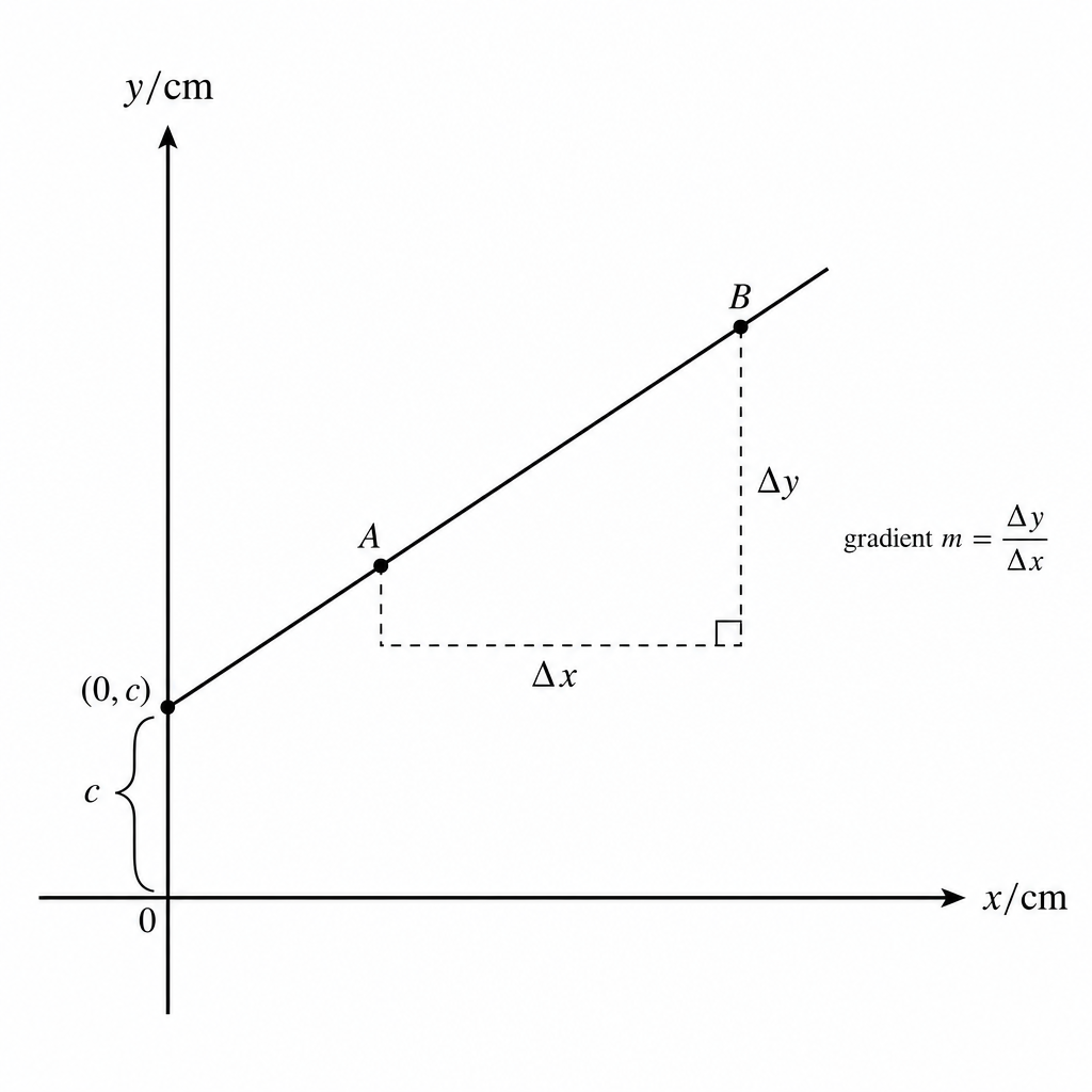
Pick two points on the line with a large horizontal separation (large $\Delta x$ ) so that small reading errors have less effect.
Read $(x_1,y_1)$ and $(x_2,y_2)$ from the axes, keeping the same units as your graph (often $\text{cm}$ ).
Calculate:

\text{gradient} = \frac{y_2-y_1}{x_2-x_1}

To find the intercept, extend the line back to meet the $y$ -axis (where $x=0$ ) and read off $y$ .

Note: If your axes are in $\text{cm}$ , then the gradient has unit $\text{cm cm}^{-1}$ , i.e. it is dimensionless.

Key Takeaways

Use the best-fit line, not point-to-point differences.
Use a large triangle for the gradient.
Intercept is the value at $x=0$ .

Common Mistakes

Using two data points that are close together (large percentage uncertainty).
Calculating $\Delta x / \Delta y$ instead of $\Delta y / \Delta x$ .
Forgetting that intercept must come from the line, not the nearest plotted point.

Things to Be Careful About

Keep units consistent throughout; if the axes are in $\text{cm}$ then keep $x$ and $y$ in $\text{cm}$ for the gradient calculation.
Read coordinates carefully (avoid parallax when reading the graph).
Extend the best-fit line lightly in pencil to reach the $y$ -axis if needed.

Techniques used

use two well-separated points on the best-fit linecalculate the gradient using \u0394y/\u0394xread the y-intercept from the graph at x = 0

(e)

It is suggested that the quantities $y$ and $x$ are related by the equation

y = Px + Q

where $P$ and $Q$ are constants.

Using your answers in (d)(iii), determine the values of $P$ and $Q$ . Give appropriate units.

$P$ = ______
$Q$ = ______

DifficultyMedium-Easy

Worked solution

Given

y = Px + Q

Comparing with $y = mx + c$ :

P = \text{gradient}

Q = \text{$y$-intercept}

Using (d)(iii) (example):

P = 0.900\ (\text{no unit})

Q = 30.0\ \text{cm}

Final answer

P = gradient (dimensionless), Q = y-intercept (length unit of y).

Detailed explanation

Background Concept

A straight-line relationship can always be written as

y = mx + c

where $m$ is the gradient and $c$ is the intercept. If the question uses different letters (here $P$ and $Q$ ), you identify them by matching the algebraic form.

Units:

If $y$ and $x$ are both lengths measured in the same unit, then $P$ has unit $\text{(length)}/\text{(length)}$ which cancels, so $P$ is dimensionless.
$Q$ has the same unit as $y$ .

Understanding the Question

You are told that

y = Px + Q

and you have already found a gradient and intercept from your graph. You must state $P$ and $Q$ (with units).

Approach

Recognise that the plotted graph is $y$ against $x$ , so it matches the straight line form.
Set $P$ equal to the measured gradient.
Set $Q$ equal to the measured $y$ -intercept.
Attach appropriate units based on what you used on the axes.

Step-by-Step Reasoning

From (d)(iii) you have a value of gradient $m$ .
Comparing forms term-by-term:
- coefficient of $x$ is the gradient, so $P=m$ ,
- constant term is the intercept, so $Q=c$ .
If you plotted $x$ and $y$ in $\text{cm}$ , then $Q$ is in $\text{cm}$ .

Key Takeaways

Matching to $y = mx + c$ is the standard way to interpret gradients/intercepts.
Units follow directly from the axis units.

Common Mistakes

Swapping $P$ and $Q$ .
Giving $P$ the unit $\text{cm}$ (it should be dimensionless if both axes are cm).
Using a value from a single data point instead of the best-fit line values.

Things to Be Careful About

If you used different units on axes (e.g. $x$ in m and $y$ in cm), then $P$ would carry units; normally you should keep both as the same length unit.
Quote values to a sensible number of significant figures consistent with graph reading precision.

Techniques used

compare the experimental line equation with y = mx + cidentify constants from gradient and interceptassign appropriate units to constants

(f)

Theory suggests that

P = \frac{2m}{(R+m)}

where $R$ is the mass of the metre rule and $m = 0.100\text{ kg}$ .

Calculate $R$ . Give your answer to three significant figures.

$R$ = ______ $\text{kg}$

DifficultyMedium

Worked solution

Working

Given

P = \frac{2m}{(R+m)}

Rearrange:

P(R+m) = 2m

PR + Pm = 2m

PR = m(2-P)

R = \frac{m(2-P)}{P} = \frac{2m}{P} - m

Using $m = 0.100\ \text{kg}$ and (example) $P = 0.900$ :

R = \frac{2(0.100)}{0.900} - 0.100 = 0.122\ \text{kg}

Answer

R = 0.122\ \text{kg}

Final answer

R = 0.122 kg (example, using P = 0.900)

Detailed explanation

Background Concept

When theory links an experimental gradient/constant to a physical parameter, you combine:

your experimental determination of a constant (here $P$ from the graph),
the theoretical relationship (here involving $R$ and $m$ ),
algebraic rearrangement to solve for the unknown.

Significant figures: the question explicitly requests three significant figures for $R$ .

Understanding the Question

You are given

P = \frac{2m}{(R+m)}

with $m = 0.100\ \text{kg}$ . You found $P$ from your graph in (e). You must calculate $R$ , the mass of the metre rule, to three significant figures.

Approach

Make $R$ the subject of the equation.
Substitute $m$ and your measured $P$ .
Round to three significant figures and include units of $\text{kg}$ .

Step-by-Step Reasoning

Starting with

P = \frac{2m}{R+m}

Multiply both sides by $(R+m)$ :

P(R+m) = 2m

Expand brackets:

PR + Pm = 2m

Rearrange to isolate $PR$ :

PR = 2m - Pm = m(2-P)

Divide by $P$ :

R = \frac{m(2-P)}{P}

A useful equivalent form is:

R = \frac{2m}{P} - m

Then substitute $m=0.100\ \text{kg}$ and your $P$ value from the graph. Finally, round to three significant figures.

Key Takeaways

Practical graphs often provide constants that feed into a theoretical equation.
Clean algebra (making the correct variable the subject) is essential.
Always include the unit and the requested significant figures.

Common Mistakes

Using the intercept $Q$ instead of the gradient $P$ .
Algebra errors when rearranging (especially with brackets in the denominator).
Rounding too early and losing accuracy.

Things to Be Careful About

Use your own experimentally determined $P$ from (e), not the example value.
Ensure $P$ is dimensionless (if $x$ and $y$ used the same length unit), so $R$ comes out in $\text{kg}$ .
Round the final $R$ to three significant figures exactly as asked.

Techniques used

rearrange an algebraic relationship to make the required variable the subjectsubstitute experimental gradient and given mass valueround the final value to the required significant figures

The rest of this paper

1 more questions

Q2Manipulation, Measurement and Observation · Analysis, Conclusions and Evaluation · Presentation of Data and Observations20M

Loading the full paper…