In this experiment, you will investigate an electrical circuit. You are provided with groups of components connected in parallel. The circuit symbol for each of these components is shown in Fig. 1.1. (a) • Assemble the circuit shown in Fig. 1.2. • Check that the positive terminals of the power supply, component C and the groups of components are connected as shown in Fig. 1.2. • Connect the movable lead L to terminal A. • Close the switch S. • Record the voltage $V_S$ shown…

(a) V_S ≈ 3.00 V · (b) n and V recorded (student-dependent) · (c) Table of six (n, V) values with 1/V calculated (student-dependent) · (d)(i) Graph of 1/V (y) against n (x) plotted · (d)(ii) Straight line of best fit drawn · (d)(iii) gradient ≈ 0.090 V^-1, y-intercept ≈ 0.25 V^-1 · (e) a ≈ 0.090 V^-1, b ≈ 0.25 V^-1

Physics 9702/34 — May/June 2018

Cambridge AS Level · Advanced Practical Skills · worked solutions for every part, with the mark scheme

questions

marks

120

minutes

Topics Manipulation, Measurement and Observation · Presentation of Data and Observations · Analysis, Conclusions and Evaluation

Q1Manipulation, Measurement and ObservationPresentation of Data and ObservationsAnalysis, Conclusions and EvaluationFree sample

In this experiment, you will investigate an electrical circuit.

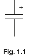
You are provided with groups of components connected in parallel. The circuit symbol for each of these components is shown in Fig. 1.1.

Fig. 1.1

(a)

• Assemble the circuit shown in Fig. 1.2.

Fig. 1.2

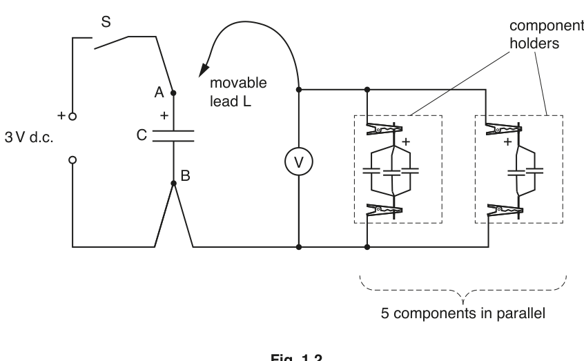
• Check that the positive terminals of the power supply, component C and the groups of components are connected as shown in Fig. 1.2.
• Connect the movable lead L to terminal A.
• Close the switch S.
• Record the voltage $V_S$ shown on the voltmeter.

$V_S$ = ______

• Open switch S.

DifficultyEasy

Worked solution

Answer

A typical measured supply voltage is

V_S = 3.00\ \text{V}

Final answer

V_S ≈ 3.00 V

Detailed explanation

Background Concept

A voltmeter measures the potential difference (p.d.) between two points in a circuit. For a d.c. power supply, this p.d. should be approximately constant when the circuit is connected correctly. In practical work, the key skills are (i) assembling exactly as the circuit diagram shows, and (ii) reading the meter correctly (including polarity).

Understanding the Question

You are told to build the circuit of Fig. 1.2, ensure the positive terminals are connected as shown, connect the movable lead $L$ to terminal $A$ , close the switch, and record the supply voltage $V_S$ shown on the voltmeter. This is simply a measurement check that the supply p.d. is what it should be.

Approach

Assemble the circuit carefully and check polarities (especially for polarised components).
With $L$ at $A$ and switch $S$ closed, wait for the voltmeter reading to settle.
Record $V_S$ to the resolution of the voltmeter.

Step-by-Step Reasoning

Connect the circuit exactly as in Fig. 1.2.
Confirm the positive terminals are consistent (misconnection can give a negative reading or damage a polarised capacitor).
Set $L$ to terminal $A$ .
Close $S$ so the supply is connected.
Read the voltmeter value and record it (e.g. $3.00\ \text{V}$ if the meter reads to $0.01\ \text{V}$ ).
Open $S$ as instructed.

Key Takeaways

Correct circuit assembly and polarity checking are essential before taking data.
Record meter readings with appropriate precision and units.

Common Mistakes

Reversing polarity of a polarised capacitor (may give wrong readings or risk damage).
Recording $V_S$ without units.
Writing too many/few decimal places compared with the voltmeter resolution.

Things to Be Careful About

Ensure $L$ is connected to the correct terminal ( $A$ for this step).
Read the voltmeter directly (avoid parallax if it is an analogue scale).
If the reading fluctuates, record a stable value (or note instability if it persists).

Techniques used

assemble the circuit according to a given diagramcheck component polarity and correct connectionsread a voltmeter value at steady conditions

(b)

• Record the total number $n$ of components in parallel in the component holders.

$n$ = ______

• Move the movable lead L and connect it to terminal B.
• Close switch S.
• Open switch S after approximately 5 s.
• Move the movable lead L and connect it to terminal A. Immediately record the voltage $V$ shown on the voltmeter.

$V$ = ______

DifficultyMedium-Easy

Worked solution

Answer

Total number of components in parallel (from the holders), e.g.

n = 2

Voltage recorded immediately after returning $L$ to $A$ , e.g.

V = 2.26\ \text{V}

Final answer

n and V recorded (student-dependent)

Detailed explanation

Background Concept

In time-dependent circuits (especially involving capacitors), voltages can change after switching because charge redistributes. That is why instructions often include a fixed charging time (here about $5\ \text{s}$ ) and the word “IMMEDIATELY” when taking a reading.

Understanding the Question

You must:

record $n$ , the total number of components connected in parallel in the holders,
then change $L$ to $B$ , close $S$ for about $5\ \text{s}$ , open $S$ ,
move $L$ back to $A$ and immediately read $V$ .
The key point is that the reading must be taken straight away, because $V$ can drift after switching.

Approach

Count all components actually in parallel in the holders to obtain $n$ .
Perform the switching sequence with approximately the same $5\ \text{s}$ timing each time.
When told to record $V$ immediately, have your eyes on the meter before you move the lead so you can read without delay.

Step-by-Step Reasoning

Determine $n$ by counting the components in each holder and adding them.
Connect $L$ to $B$ and close $S$ .
Use a stopwatch/clock to estimate $5\ \text{s}$ (consistent timing matters for repeatability).
Open $S$ after about $5\ \text{s}$ .
Move $L$ back to $A$ .
Immediately read $V$ on the voltmeter and record it with unit and correct precision.

Key Takeaways

In practical electricity questions, repeatability depends on consistent timing and consistent switching.
“Immediately” is a mark-scheme hint: delays increase scatter in the graph.

Common Mistakes

Forgetting to include all components when calculating $n$ .
Leaving switch $S$ closed too long or too short compared with other runs.
Recording $V$ after a delay (reading no longer corresponds to the intended condition).

Things to Be Careful About

Keep the $5\ \text{s}$ as consistent as possible for every value of $n$ .
Record $V$ to the voltmeter resolution (e.g. $2.3\ \text{V}$ vs $2.30\ \text{V}$ depending on the meter).
Ensure $L$ makes a good electrical contact at terminals $A$ and $B$ each time.

Techniques used

count the number of components connected in parallelfollow a timed switching sequence consistentlyrecord a meter reading immediately after a circuit change

(c)

Change $n$ and repeat (b) until you have six sets of values of $n$ and $V$ . One of the component holders may be left empty if required.

Record your results in a table. Include your values from (b). Also include values of $\frac{1}{V}$ in your table.

DifficultyMedium

Worked solution

Answer

Record six sets of $n$ and $V$ in one table and calculate $\dfrac{1}{V}$ for each row.

Example of a correctly laid-out table (values are illustrative):

$n$	$V\,/\,\text{V}$	$\dfrac{1}{V}\,/\,\text{V}^{-1}$
1	2.94	0.340
2	2.33	0.429
3	1.92	0.521
4	1.64	0.610
5	1.43	0.699
6	1.27	0.787

(Include your value from (b); keep $V$ recorded to consistent precision and $1/V$ calculated accordingly.)

Final answer

Table of six (n, V) values with 1/V calculated (student-dependent)

Detailed explanation

Background Concept

Good experimental data presentation means:

one clear table containing all readings,
column headings that show the quantity and unit,
consistent decimal places/significant figures in a column,
correct calculation of any derived quantities (here $1/V$ ).
For a reciprocal, the unit also inverts: if $V$ is in $\text{V}$ then $1/V$ is in $\text{V}^{-1}$ .

Understanding the Question

You must change $n$ and repeat the procedure from (b) until you have six pairs of values $(n, V)$ . You then need a results table that includes these and an extra column for $1/V$ .

Approach

Choose six different values of $n$ (a good spread, e.g. from small to large $n$ ).
For each $n$ , carry out exactly the same switching/timing steps and record $V$ .
Fill a single table with columns: $n$ , $V$ , and $1/V$ .
Calculate $1/V$ using a calculator and present it to a sensible number of significant figures (usually 3 s.f. is fine unless your raw data is less precise).

Step-by-Step Reasoning

Decide the set of $n$ values you will use. The independent variable is $n$ , so you must vary it systematically and record the corresponding dependent variable $V$ .
Perform the measurement sequence each time (same approximate $5\ \text{s}$ time, and read $V$ immediately).
Construct a table:
- First column: $n$ (dimensionless, so no unit).
- Second column: $V\,/\,\text{V}$ .
- Third column: $1/V\,/\,\text{V}^{-1}$ .
For each row, compute

\frac{1}{V}

using your recorded $V$ for that row.

Check that your $1/V$ values are consistent with your $V$ values (larger $V$ should give smaller $1/V$ and vice versa).

Key Takeaways

A practical table must be complete (all six data sets), neat, and correctly labelled.
Derived quantities must have correct units and appropriate significant figures.

Common Mistakes

Missing units in column headings (e.g. writing just $V$ instead of $V\,/\,\text{V}$ ).
Inconsistent precision in the $V$ column (mixing $2.3$ and $2.31$ without justification).
Calculating $1/V$ but not stating the unit $\text{V}^{-1}$ .
Not collecting a sufficient range of $n$ values (values too clustered reduce graph quality).

Things to Be Careful About

Do not round $V$ excessively before calculating $1/V$ ; use the measured $V$ .
Keep the same method and timing for every $n$ to reduce scatter.
If one holder is empty, ensure $n$ correctly reflects the total components actually connected.

Techniques used

vary the independent variable over a suitable rangerecord results in a single table with correct headings and unitscalculate a derived quantity for each rowuse consistent significant figures within columns

(d)

(i)

Plot a graph of $\frac{1}{V}$ on the $y$ -axis against $n$ on the $x$ -axis.

DifficultyMedium-Easy

Worked solution

Answer

Plot $\dfrac{1}{V}$ on the $y$ -axis and $n$ on the $x$ -axis.

Label axes: $n$ (no unit) and $1/V\,/\,\text{V}^{-1}$ .
Use a scale that uses at least half the graph grid on each axis.
Plot all six points accurately.

Final answer

Graph of 1/V (y) against n (x) plotted

Detailed explanation

Background Concept

A graph is used to reveal trends and test whether a relationship is linear. For full credit in Paper 3 graph marks, you must:

choose appropriate axes (correct variables),
label axes with quantities and units,
use sensible scales (not cramped; not awkward like 3 squares = 1 unit),
plot points precisely.

Understanding the Question

You are instructed to plot a graph with $1/V$ on the $y$ -axis and $n$ on the $x$ -axis. Your table from (c) provides the coordinates $(n, 1/V)$ .

Approach

Draw axes and decide scales that spread your data across the page.
Label axes properly.
Plot each point from the table using sharp pencil marks (small crosses).

Step-by-Step Reasoning

Put $n$ on the horizontal axis because it is the independent variable you controlled.
Put $1/V$ on the vertical axis because it is the derived dependent variable you calculated.
Choose the range: from your smallest to largest $n$ , and smallest to largest $1/V$ .
Choose scales so that the plotted points occupy most of the graph area.
Plot each point carefully; a typical convention is a cross of size about half a small square.

Key Takeaways

Correct axis labels and sensible scales are as important as correct plotting.
Independent variable on $x$ , dependent on $y$ .

Common Mistakes

Plotting $V$ instead of $1/V$ .
Missing units on the $1/V$ axis.
Using a scale that is too small (points bunched together) or too awkward.
Plotting fewer than six points.

Things to Be Careful About

$n$ is dimensionless: do not write a unit for it.
Make sure you use the same $1/V$ values as in your table (avoid recalculating differently and introducing rounding inconsistencies).

Techniques used

label graph axes with quantity and unitchoose a sensible linear scale using most of the gridplot points accurately from a table

(ii)

Draw the straight line of best fit.

DifficultyEasy

Worked solution

Answer

Draw a single straight line of best fit so that the points are distributed approximately evenly about the line (do not join dot-to-dot).

Final answer

Straight line of best fit drawn

Detailed explanation

Background Concept

A best-fit line represents the overall trend of experimental data when scatter is present. For a relationship expected to be linear, you draw one straight line that balances the points above and below it.

Understanding the Question

After plotting $1/V$ against $n$ , you must draw the straight line of best fit.

Approach

Use a ruler to draw one straight line that follows the trend and has roughly equal scatter of points on either side.

Step-by-Step Reasoning

Look for the general trend of your plotted points.
Place a ruler so that it lies close to as many points as possible, with a similar number of points above and below.
Draw a single straight line across the full range of your data.

Key Takeaways

Best-fit is about the overall pattern, not passing through every point.

Common Mistakes

Joining points dot-to-dot.
Forcing the line through the origin when it does not suit the data.
Drawing a line only through the middle points and not extending across the plotted range.

Things to Be Careful About

Use a sharp pencil and a thin line.
If one point is clearly anomalous, you still normally draw the best-fit line for the overall data unless instructed otherwise.

Techniques used

judge the overall trend of plotted pointsdraw a straight line of best fit with balanced scatterignore minor point-to-point fluctuations

(iii)

Determine the gradient and $y$ -intercept of this line.

gradient = ______
$y$ -intercept = ______

DifficultyMedium-Easy

Worked solution

Working

Using two points on the best-fit line (well separated), e.g.

(n_1, y_1) = (1,\ 0.34\ \text{V}^{-1}),\quad (n_2, y_2) = (6,\ 0.79\ \text{V}^{-1})

\text{gradient } m = \frac{\Delta y}{\Delta x} = \frac{0.79 - 0.34}{6 - 1} = 0.090\ \text{V}^{-1}

From the best-fit line at $n = 0$ ,

\text{y-intercept } c \approx 0.25\ \text{V}^{-1}

Answer

\text{gradient} = 0.090\ \text{V}^{-1}

y\text{-intercept} = 0.25\ \text{V}^{-1}

Final answer

gradient ≈ 0.090 V^-1, y-intercept ≈ 0.25 V^-1

Detailed explanation

Background Concept

For a straight-line graph of $y$ against $x$ , the gradient is

\text{gradient} = \frac{\Delta y}{\Delta x}

and the $y$ -intercept is the value of $y$ when $x = 0$ . Gradient units are the units of $y$ divided by the units of $x$ .

Here, $y = 1/V$ (unit $\text{V}^{-1}$ ) and $x = n$ (dimensionless), so the gradient and intercept both have unit $\text{V}^{-1}$ .

Understanding the Question

You must use your best-fit line on the $1/V$ vs $n$ graph to find:

the gradient of the line,
the $y$ -intercept (where the line crosses the $y$ -axis).
These are read from the drawn best-fit line, not from individual data points.

Approach

Choose two points on the best-fit line far apart (to reduce percentage reading error).
Read their coordinates $(n_1, y_1)$ and $(n_2, y_2)$ .
Compute $m = (y_2-y_1)/(n_2-n_1)$ .
Read the $y$ -intercept by extending the best-fit line to $n=0$ .

Step-by-Step Reasoning

Pick two points that lie on the line (not necessarily measured points), ideally near the ends of the plotted range.
Read $n_1, y_1$ and $n_2, y_2$ carefully from the axes.
Calculate the differences:

\Delta y = y_2 - y_1,\quad \Delta x = n_2 - n_1

Then:

m = \frac{\Delta y}{\Delta x}

For the intercept, either read directly where the line crosses the $y$ -axis, or use $y = mx + c$ with one point on the line:

c = y - mx

Quote sensible significant figures (often 2 or 3 s.f.) consistent with graph-reading precision.

Key Takeaways

Always take gradient from the best-fit line using widely separated points.
Units: gradient has $\text{V}^{-1}$ because $n$ has no unit.

Common Mistakes

Using two adjacent points (gives a large uncertainty in gradient).
Using plotted data points rather than points on the best-fit line.
Calculating gradient as $\Delta x/\Delta y$ instead of $\Delta y/\Delta x$ .
Forgetting units on gradient/intercept.

Things to Be Careful About

Read coordinates carefully: small axis-reading errors strongly affect gradient.
Ensure you use the same axes quantities ( $y = 1/V$ , $x = n$ ).
Do not assume the intercept is zero unless your line clearly supports it.

Techniques used

select two well-separated points on the best-fit linecalculate gradient using \Delta y/\Delta xread the y-intercept from the graph

(e)

It is suggested that the quantities $V$ and $n$ are related by the equation

\frac{1}{V} = an + b

where $a$ and $b$ are constants.

Use your answers in (d)(iii) to determine the values of $a$ and $b$ . Give appropriate units.

$a$ = ______
$b$ = ______

DifficultyMedium-Easy

Worked solution

Working

Given

\frac{1}{V} = an + b

Comparing with $y = mx + c$ for a graph of $y = 1/V$ against $x = n$ :

a = \text{gradient},\quad b = \text{y-intercept}

Answer

a = 0.090\ \text{V}^{-1}

b = 0.25\ \text{V}^{-1}

Final answer

a ≈ 0.090 V^-1, b ≈ 0.25 V^-1

Detailed explanation

Background Concept

If experimental data is consistent with a linear equation

y = mx + c

then a graph of $y$ against $x$ should be a straight line, with:

gradient $m$ ,
$y$ -intercept $c$ .
By matching symbols, you can identify physical constants from the measured gradient and intercept.

Understanding the Question

You are told the suggested relationship is

\frac{1}{V} = an + b

and you have already found the gradient and intercept of the graph of $1/V$ (y-axis) against $n$ (x-axis). You must now state $a$ and $b$ (with units).

Approach

Match the equation to the straight-line form by identifying:

$y \equiv 1/V$ ,
$x \equiv n$ ,
so the coefficient of $n$ is the gradient and the constant term is the intercept.

Step-by-Step Reasoning

Your plotted graph has vertical axis $1/V$ and horizontal axis $n$ , so it represents

y = an + b

with $y = 1/V$ .

Therefore:

a = \text{gradient of the best-fit line}

and

b = \text{value of } \frac{1}{V} \text{ when } n = 0

Units:
- $n$ has no unit, so $a$ must have the same unit as $1/V$ , which is $\text{V}^{-1}$ .
- $b$ is also a value of $1/V$ , so it is $\text{V}^{-1}$ .

Key Takeaways

When you plot the variables exactly as in a linear equation, the gradient and intercept give the constants immediately.
Always state units: here both constants have unit $\text{V}^{-1}$ .

Common Mistakes

Swapping $a$ and $b$ .
Giving $a$ unit $\text{V}^{-1}\ \text{component}^{-1}$ (not needed because $n$ is dimensionless).
Quoting too many significant figures that are not justified by graph-reading.

Things to Be Careful About

Ensure the graph you used is $1/V$ vs $n$ (not $V$ vs $n$ ).
Use your measured gradient/intercept values, not values calculated from individual table entries.

Techniques used

match an experimental graph to the form y = mx + cidentify constants from gradient and interceptassign correct units using dimensional reasoning

The rest of this paper

1 more questions

Q2Manipulation, Measurement and Observation · Analysis, Conclusions and Evaluation · Presentation of Data and Observations20M

Loading the full paper…