Physics 9702/33 — October/November 2017

Cambridge AS Level · Advanced Practical Skills · worked solutions for every part, with the mark scheme

questions

marks

120

minutes

Topics Manipulation, Measurement and Observation · Presentation of Data and Observations · Analysis, Conclusions and Evaluation

Q120MManipulation, Measurement and ObservationPresentation of Data and ObservationsAnalysis, Conclusions and EvaluationFree sample

In this experiment, you will investigate the rotational motion of a mass.

(a)

You have been provided with a $10\text{ g}$ mass hanger and several $10\text{ g}$ slotted masses.

Set up the apparatus as shown in Fig. 1.1.

Fig. 1.1

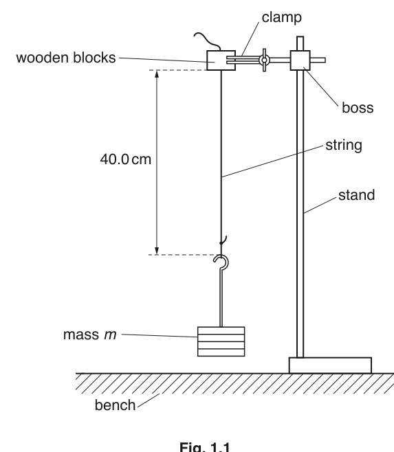
Adjust the string so that the distance between the bottom of the wooden blocks and the top of the mass hanger is $40.0\text{ cm}$ .

The combined mass $m$ of the mass hanger and slotted masses must be $70\text{ g}$ .

DifficultyMedium-Easy

Worked solution

Answer

Attach slotted masses so that the total mass is

m = 70\ \text{g}

Adjust the string so that the distance between the bottom of the wooden blocks and the top of the mass hanger is

40.0\ \text{cm}.

Final answer

Apparatus set with distance = 40.0 cm and m = 70 g.

Detailed explanation

Background Concept

In Paper 3 practical questions, marks are awarded for following instructions accurately and using measuring instruments properly. Here, two key set conditions are required:

a fixed length (string length between two reference points)
a fixed total mass (hanger + added slotted masses)

Correct set-up matters because changing either the length of the string or the total mass changes the rotational motion and therefore the times measured later.

Understanding the Question

You are told to set up the apparatus like Fig. 1.1, then:

set the distance from the bottom of the wooden blocks to the top of the mass hanger to (40.0\ \text{cm})
ensure the combined mass (m) of the hanger plus slotted masses is (70\ \text{g})

This part is essentially an instruction-check: if these are wrong, all later readings will be inconsistent.

Approach

Assemble the stand, clamp, wooden blocks, and string exactly as shown.
Use a ruler to set the specified distance between the stated reference points.
Add slotted masses to the hanger until the total mass is (70\ \text{g}).

Step-by-Step Reasoning

The mass hanger is (10\ \text{g}). To make (m=70\ \text{g}), you must add (60\ \text{g}) of slotted masses (e.g. six (10\ \text{g}) masses).
Measure the vertical distance from the bottom of the wooden blocks to the top of the mass hanger. These reference points are chosen so that the same length is used every time.
Adjust the string (by pulling through the blocks / repositioning as allowed by the set-up) until the ruler reading is (40.0\ \text{cm}). A reading of (40.0\ \text{cm}) implies you should set it to the nearest (0.1\ \text{cm}).

Key Takeaways

Follow the diagram and the stated reference points exactly.
Combine masses correctly to reach a required total.
Record/set lengths to the precision implied by the question.

Common Mistakes

Using the wrong points for the (40.0\ \text{cm}) measurement (e.g. measuring to the bottom of the hanger).
Forgetting the hanger mass is part of (m).
Setting (40\ \text{cm}) rather than (40.0\ \text{cm}) (loss of expected precision).

Things to Be Careful About

Ensure the string hangs freely and is not rubbing significantly on the wooden blocks.
Keep the ruler aligned with the string (avoid parallax by reading at eye level).
Make sure the masses are secure so (m) does not change during the run.

Techniques used

assemble the apparatus to match a given diagrammeasure a fixed length with a ruler and set it accuratelycombine slotted masses to obtain a required total mass

(b)

(i)

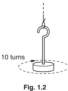
Twist the mass through ten complete turns as shown in Fig. 1.2.

Fig. 1.2

DifficultyEasy

Worked solution

Answer

Twist the mass hanger through

10

complete turns.

Final answer

10 complete turns.

Detailed explanation

Background Concept

For oscillatory/rotational experiments, the initial conditions (how far you twist or displace the system) must be controlled. Using the same number of turns each time ensures a fair comparison between different masses and string lengths.

Understanding the Question

You are instructed to twist the mass through ten complete turns (as indicated in Fig. 1.2). This sets the same starting twist before releasing the mass.

Approach

Rotate the hanger while counting full revolutions.
Stop exactly at 10 turns so each run starts from the same twist.

Step-by-Step Reasoning

A “complete turn” means one full revolution, returning to the same orientation.
Count aloud (or use a mark on the hanger/string) to avoid losing count.
Ensure the string is twisted, not the stand/clamp slipping.

Key Takeaways

Consistent initial twist improves reliability and reduces scatter in timing results.

Common Mistakes

Counting half-turns incorrectly.
Letting the clamp or blocks rotate slightly instead of twisting only the string.

Things to Be Careful About

Make sure the string remains in the same position between the blocks so frictional conditions are similar each run.
Do not stretch the string by pulling downward while twisting (changes length/tension).

Techniques used

apply a specified initial displacement to a systemcount complete rotations consistentlyprepare the system for a timed run

(ii)

When the mass is released, it will rotate one way and then rotate the other way. This motion will continue until the mass comes to rest. At this point, the mass will continue to swing slightly with very little rotation.

Release the mass. Measure and record the time $a$ taken for the mass to come to rest.

$a$ = ______

DifficultyMedium-Easy

Worked solution

Answer

Start the stopwatch on release and stop it when the mass first comes to rest (after the rotations die away).

Example reading:

a = 19.9\ \text{s}

Final answer

a ≈ 19.9 s (example; student-dependent).

Detailed explanation

Background Concept

Timing in practical physics is limited by reaction time and by how clearly you can define the start and end of the event being timed. To obtain good quality data:

define an unambiguous start (here: the instant the mass is released)
define an unambiguous end (here: the instant rotational motion has ceased and it is essentially only swinging slightly)
repeat measurements to reduce random error

Understanding the Question

After twisting 10 turns and releasing, the mass rotates one way then the other, gradually losing energy due to friction and air resistance. You must measure the time (a) from release until it “comes to rest” (i.e. rotation has died away).

Approach

Use a stopwatch.
Start timing at the instant of release.
Watch for the point where rotation is no longer occurring (only small swinging).
Ideally repeat and average if time allows.

Step-by-Step Reasoning

Hold the hanger at the 10-turn starting position.
Release without pushing (a push changes the motion and makes results inconsistent).
Start the stopwatch at the moment of release.
Observe the hanger: it will rotate alternately in opposite directions with decreasing amplitude.
Stop the stopwatch at the moment the hanger ceases rotating and only swings slightly.
Record (a) to the stopwatch resolution (typically (0.1\ \text{s}) for a digital stopwatch).
If repeating: take at least two or three readings and calculate a mean (a).

Key Takeaways

Define the end-point consistently across trials.
Repeats reduce random timing scatter.

Common Mistakes

Stopping when rotation becomes slow rather than when it has stopped.
Starting/stopping late due to distraction or poor viewpoint.
Not recording the unit or recording to an unrealistic precision.

Things to Be Careful About

Keep your eye level consistent to avoid misjudging whether rotation is still occurring.
If the end-point is hard to judge, use a consistent rule (e.g. “stop when the hanger does not complete any further visible fraction of a turn”).
Do not let the hanger hit the bench; that produces an abrupt stop not related to the intended damping.

Techniques used

time an event using a stopwatch with a clear start and end conditionidentify the end-point of motion consistentlyrepeat timing measurements and take a mean

(iii)

Change the distance between the bottom of the wooden blocks and the top of the mass hanger to $20.0\text{ cm}$ .

DifficultyEasy

Worked solution

Answer

Adjust the string so the distance between the bottom of the wooden blocks and the top of the mass hanger is

20.0\ \text{cm}.

Final answer

Distance set to 20.0 cm.

Detailed explanation

Background Concept

In experiments, you often change one variable while keeping others constant. Here, the string length (between specified points) is changed from (40.0\ \text{cm}) to (20.0\ \text{cm}) while keeping the same total mass (m) for the next run.

Understanding the Question

You must adjust the apparatus so that the same measured distance (bottom of wooden blocks to top of mass hanger) becomes (20.0\ \text{cm}). This prepares the system for timing (b) in the next step.

Approach

Use the ruler to measure the same reference points as before.
Adjust until the length is (20.0\ \text{cm}), maintaining the rest of the set-up unchanged.

Step-by-Step Reasoning

Locate the bottom edge of the wooden blocks (reference point 1).
Locate the top of the mass hanger (reference point 2).
Slide/adjust the string appropriately and re-check the measurement.
Read the ruler at eye level to avoid parallax.

Key Takeaways

Always use the same reference points when setting a length.

Common Mistakes

Measuring from the wrong point on the hanger.
Forgetting to re-check after tightening the clamp/blocks.

Things to Be Careful About

Ensure the string is vertical when measuring.
Keep (m) unchanged during this length adjustment step.

Techniques used

reset an experimental variable to a specified valuemeasure a fixed length between defined reference pointsmaintain consistent set-up while changing one parameter

(iv)

Repeat (b)(i).

Release the mass. Measure and record the time $b$ taken for the mass to come to rest.

$b$ = ______

DifficultyMedium-Easy

Worked solution

Answer

Twist 10 turns, release, then time until the mass comes to rest.

Example reading:

b = 12.0\ \text{s}

Final answer

b ≈ 12.0 s (example; student-dependent).

Detailed explanation

Background Concept

To compare two conditions (here, different string lengths), the procedure must be identical except for the variable changed. The timing uncertainty is largely random (reaction time), so consistent technique and repeats improve reliability.

Understanding the Question

With the distance now (20.0\ \text{cm}), you repeat the 10-turn twist and release, and measure the time (b) until the rotational motion dies away.

Approach

Use the same start/end definitions as for (a).
Record (b) to the same precision as (a).
Repeat and average if possible.

Step-by-Step Reasoning

Twist the mass through 10 complete turns.
Release without an extra push.
Start timing at release.
Observe the rotations decreasing until rotation stops.
Stop timing at the same “comes to rest” criterion used for (a).
Record (b) (typically to (0.1\ \text{s})).

Key Takeaways

Fair tests: same method, only one variable changed.

Common Mistakes

Using a different end-point criterion than for (a).
Recording (b) to different decimal places than (a).

Things to Be Careful About

Ensure the length is truly (20.0\ \text{cm}) when timing (b).
If the hanger swings and makes judging rotation difficult, view from above/side consistently and apply the same rule each time.

Techniques used

repeat the same timing procedure under changed conditionstime until a defined endpoint is reachedrecord measurements to appropriate resolution

(v)

Change the distance between the bottom of the wooden blocks and the top of the mass hanger to $40.0\text{ cm}$ .

DifficultyEasy

Worked solution

Answer

Reset the distance to

40.0\ \text{cm}.

Final answer

Distance reset to 40.0 cm.

Detailed explanation

Background Concept

When multiple trials are required, returning to a standard configuration reduces systematic differences between runs and helps ensure each new dataset is comparable.

Understanding the Question

After measuring (b) at (20.0\ \text{cm}), you are told to change the distance back to (40.0\ \text{cm}) ready for the next set of readings in part (c).

Approach

Adjust the string back to the original length using the same reference points.

Step-by-Step Reasoning

Measure from the bottom of the wooden blocks to the top of the mass hanger.
Adjust until the reading is (40.0\ \text{cm}).
Ensure nothing else has changed (masses still secure; clamp still firm).

Key Takeaways

Use consistent reference points and precision each time you set a length.

Common Mistakes

Setting (40\ \text{cm}) rather than (40.0\ \text{cm}).

Things to Be Careful About

Check that the hanger is not oscillating while you set the length; set it when stationary for an accurate measurement.

Techniques used

reset an experimental condition to its original valuecheck a measurement after adjustmentmaintain consistent apparatus geometry

(c)

Change $m$ and repeat (b) until you have six sets of values of $m$ , $a$ and $b$ . You may include your results from (b).

Record your results in a table. Include values of $\frac{a^2}{b}$ in your table.

10M

DifficultyMedium-Hard

Worked solution

Answer

Record six sets of (m), (a), (b) and calculate (\dfrac{a^2}{b}). Headings must include quantity and unit.

Example table (illustrative):

(m / \text{g})	(a / \text{s})	(b / \text{s})	(\dfrac{a^2}{b} / \text{s})
70	19.9	12.0	33.0
80	21.5	12.5	37.0
90	23.1	13.0	41.0
100	24.7	13.5	45.2
110	26.2	14.0	49.0
120	27.7	14.5	52.9

(Values shown are examples; candidate readings will vary.)

Final answer

Single table of m, a, b, and a^2/b (with units), 6 sets.

Detailed explanation

Background Concept

Practical marks for tables usually come from presentation quality and correct processing rather than matching a single “true” dataset. A good results table must:

include all raw measurements needed (here (m), (a), (b))
include the calculated quantity requested (here (a^2/b))
have clear headings with units
show consistent precision (decimal places) within each column

The derived quantity

\frac{a^2}{b}

uses time values (a) and (b), so its unit is seconds:

\frac{\text{s}^2}{\text{s}} = \text{s}.

Understanding the Question

You must change the mass (m) and repeat the timing procedure (measure (a) at (40.0\ \text{cm}) and (b) at (20.0\ \text{cm})) until you have six sets of (m, a, b). Then you must calculate (a^2/b) for each set and present everything in one table.

Approach

Choose at least six different values of (m) (e.g. in steps of (10\ \text{g})).
For each (m): measure (a) and (b) using the same method and precision.
Compute (a^2/b) for each row.
Present in one table with correct headings and units.

Step-by-Step Reasoning

Selecting (m): since you have (10\ \text{g}) slotted masses, a sensible range is, for example, (70) to (120\ \text{g}) in (10\ \text{g}) steps (six values). Any similar six-value range is acceptable as long as it is sensible and spread out.
Recording (m): keep units explicit in the heading, e.g. (m/\text{g}) (or (m/\text{kg}) if you convert). Do not mix units within the table.
Recording (a) and (b): record to the stopwatch resolution (commonly (0.1\ \text{s})). Keep the same decimal places down each time column.
Calculating (a^2/b): for each row,

\frac{a^2}{b} = \frac{(a\ \text{in s})^2}{b\ \text{in s}}

Example using one row (illustrative numbers):

\frac{a^2}{b} = \frac{(19.9)^2}{12.0} = \frac{396.0}{12.0} = 33.0\ \text{s}

Significant figures: a calculated value should normally be given to a similar precision to the raw times. If (a) and (b) are to (0.1\ \text{s}), then (a^2/b) is typically quoted to 3 s.f. (or 1 d.p. if values are around (10\text{–}100\ \text{s})). Consistency is more important than excessive precision.

Key Takeaways

Put all relevant data in one clear table.
Use correct headings: quantity / unit.
Keep consistent decimal places for raw measurements.
Check units of derived quantities.

Common Mistakes

Missing units in headings (e.g. writing just (m), (a), (b)).
Inconsistent decimal places in a column (e.g. mixing (12.0) and (12.34)).
Calculating (a^2/b) incorrectly (common error: (a/b^2) or ((a/b)^2)).
Using too few values of (m) (need six sets).

Things to Be Careful About

If you repeat timings and average them, state clearly what you recorded (mean values) and keep the same precision.
If you convert (m) to kg, do it for every row and label the column (m/\text{kg}). Converting only some values loses method marks.
When squaring (a), keep enough calculator digits until the final rounding to avoid rounding drift.

Techniques used

choose a suitable range and number of values for the independent variablerecord raw readings with units and consistent precisioncalculate a derived quantity from measured valuespresent results in a single table with correct headings

(d)

(i)

Plot a graph of $\frac{a^2}{b}$ on the $y$ -axis against $m$ on the $x$ -axis.

DifficultyMedium

Worked solution

Answer

Plot (\dfrac{a^2}{b}) on the (y)-axis against (m) on the (x)-axis.

Axes labelled (with units), suitable scales chosen, and all six points plotted accurately.

Final answer

Graph of a^2/b (y) against m (x) plotted.

Detailed explanation

Background Concept

Graph marks in Paper 3 usually reward:

correct variables on correct axes
correct axis labels including units
sensible linear scales (use at least half the grid; avoid awkward scales like 3 squares = 1 unit)
accurate plotting (small, neat crosses; correct placement)

Understanding the Question

You must plot a graph with:

(x)-axis: (m)
(y)-axis: (a^2/b)

using the six data sets you recorded in part (c).

Approach

Decide whether (m) is in g or kg based on your table, and keep that unit on the axis label.
Choose scales that spread the points well across the graph paper.
Plot each point as a small cross.

Step-by-Step Reasoning

If your masses are (for example) (70) to (120\ \text{g}), choose an (x)-axis scale such as 10 g per large square (or similar) so the points occupy much of the width.
If (a^2/b) values are (for example) (30) to (55\ \text{s}), choose a (y)-axis scale like 2 s or 5 s per large square so the points occupy much of the height.
Label axes clearly, e.g.
- (m / \text{g})
- (\left(a^2/b\right) / \text{s})
Plot each point carefully: take the x-value from the mass and the y-value from your calculated column.

Key Takeaways

Axes must include units.
Scales should be simple and use most of the grid.

Common Mistakes

Swapping axes (plotting (m) on (y) by accident).
Missing units.
Using cramped scales so points are bunched together.
Plotting blobs instead of small crosses (hard to judge line placement).

Things to Be Careful About

Do not force the graph through the origin unless the data demands it.
Ensure each plotted point corresponds to the correct row of the table (mixing up (a), (b) rows gives random scatter).

Techniques used

choose suitable axis scales that use most of the graph gridlabel axes with quantity and unitplot data points accurately from a table

(ii)

Draw the straight line of best fit.

DifficultyMedium-Easy

Worked solution

Answer

Draw a straight line of best fit through the plotted points (balanced with roughly equal scatter above and below).

Final answer

Straight line of best fit drawn.

Detailed explanation

Background Concept

A best-fit line summarises the trend in data that should follow a linear relationship. In practical work, points rarely lie exactly on a straight line due to random uncertainties, so the line should be drawn to represent the overall trend.

Understanding the Question

You have plotted (a^2/b) against (m). You are now told to draw the straight line of best fit.

Approach

Use a ruler.
Place the ruler so the line passes through the middle of the cluster of points.
Aim for roughly equal numbers of points (or equal scatter) above and below the line.

Step-by-Step Reasoning

Do not join dot-to-dot.
If one point is clearly off the general trend (an anomaly), the best-fit line should still represent the majority trend rather than being dragged to pass through the anomalous point.
Draw the line long enough that you can later read a clear intercept and choose two far-apart points on the line for the gradient calculation.

Key Takeaways

Best fit is about the overall trend, not passing through every point.

Common Mistakes

Drawing a wobbly line or a thick line.
Forcing the line through the origin.
Joining points in sequence instead of drawing a single best-fit line.

Things to Be Careful About

Use a sharp pencil; thick lines make gradient/intercept readings less accurate.
Ensure the line is straight and drawn with a ruler (freehand lines lose marks).

Techniques used

draw a single straight line that balances the scatter of pointsignore anomalous points when justified by scatterextend the best-fit line to read intercepts accurately

(iii)

Determine the gradient and $y$ -intercept of this line.

gradient = ______
$y$ -intercept = ______

DifficultyMedium

Worked solution

Working

Using two widely separated points on the best-fit line (example):

(m_1, y_1) = (70\ \text{g}, 33.0\ \text{s}),\quad (m_2, y_2) = (120\ \text{g}, 53.0\ \text{s})

\text{gradient} = \frac{\Delta y}{\Delta x} = \frac{53.0 - 33.0}{120 - 70} = \frac{20.0}{50} = 0.40\ \text{s g}^{-1}

y\text{-intercept} = y - (\text{gradient})\,m = 33.0 - (0.40)(70) = 5.0\ \text{s}

Answer

\text{gradient} = 0.40\ \text{s g}^{-1}

y\text{-intercept} = 5.0\ \text{s}

(Values shown are examples; candidate values depend on their graph.)

Final answer

gradient ≈ 0.40 s g^-1, y-intercept ≈ 5.0 s (example).

Detailed explanation

Background Concept

For a straight-line graph, the gradient (slope) and y-intercept describe the linear relationship:

y = mx + c

gradient (m = \Delta y / \Delta x)
y-intercept (c) is the value of (y) when (x = 0)

In practical exams, you must calculate the gradient using a large triangle on the best-fit line (not between two neighbouring data points), to reduce percentage reading error.

Understanding the Question

You have drawn a best-fit straight line on a graph of (y = a^2/b) against (x = m). You are asked to determine:

the gradient of this line
the y-intercept of this line

These will be used in part (e).

Approach

Choose two points far apart on the best-fit line (not necessarily measured points), and read their coordinates.
Compute

\text{gradient} = \frac{\Delta y}{\Delta x}.

Find the y-intercept either by reading where the line crosses the y-axis (if (x=0) is on the graph) or by substituting one point into (y = mx + c) to solve for (c).

Step-by-Step Reasoning

Picking points: The two points should be as far apart as possible to make (\Delta x) and (\Delta y) large, reducing the effect of a (\pm 1\ \text{mm}) reading uncertainty.
Reading coordinates: Read (m) from the x-axis and (a^2/b) from the y-axis for each chosen point.
Compute the gradient:

\text{gradient} = \frac{y_2 - y_1}{m_2 - m_1}

Include units: since (y) is in seconds and (m) is in grams (or kg), the gradient unit is (\text{s g}^{-1}) (or (\text{s kg}^{-1})).

Find y-intercept: If the graph includes (m=0), read the intercept directly. If not, use

c = y - mx

with any point ((x,y)) on the best-fit line.

Key Takeaways

Gradient is (\Delta y/\Delta x), not (\Delta x/\Delta y).
Use two widely separated points on the best-fit line.
Always state units for gradient and intercept.

Common Mistakes

Using two neighbouring plotted points, giving a poor gradient.
Calculating (\Delta x/\Delta y) by mistake.
Forgetting units or using inconsistent units (e.g. (m) in g but treating as kg).
Reading intercept from a data point instead of the line.

Things to Be Careful About

If you use (m) in kg, your gradient will be (1000) times larger than if you use g; both are fine if units match.
Do not round intermediate coordinates too aggressively; keep enough precision to get a reliable gradient.
Ensure the triangle is drawn using the best-fit line, not a segment joining two plotted points.

Techniques used

use a large triangle to calculate the gradient from a best-fit linecalculate gradient as $\Delta y / \Delta x$ with unitsdetermine the y-intercept by reading the value at $x = 0$

(e)

It is suggested that the quantities $a$ , $b$ and $m$ are related by the equation

\frac{a^2}{b} = Pm + Q

where $P$ and $Q$ are constants.

Using your answers in (d)(iii), determine the values of $P$ and $Q$ . Give appropriate units.

$P$ = ______
$Q$ = ______

DifficultyMedium-Easy

Worked solution

Working

Given

\frac{a^2}{b} = Pm + Q

This matches (y = mx + c) with

P = \text{gradient},\quad Q = y\text{-intercept}.

Using (d)(iii) (example values):

P = 0.40\ \text{s g}^{-1}

Q = 5.0\ \text{s}

Answer

P = 0.40\ \text{s g}^{-1}

Q = 5.0\ \text{s}

Final answer

P = gradient, Q = y-intercept (with units).

Detailed explanation

Background Concept

If a graph is plotted as (y) against (x) and the suggested relationship is

y = Px + Q,

then:

(P) is the gradient
(Q) is the y-intercept

Units come from the axes:

[P] = \frac{[y]}{[x]},\quad [Q] = [y].

Understanding the Question

You are told:

\frac{a^2}{b} = Pm + Q

and you have already found the gradient and y-intercept of a graph of (a^2/b) (y-axis) against (m) (x-axis). You must state (P) and (Q) with appropriate units.

Approach

Recognise that the equation is already in straight-line form.
Map:

y \equiv \frac{a^2}{b},\quad x \equiv m.

Therefore (P) is the gradient and (Q) is the intercept.
Assign units based on what units you used for (m).

Step-by-Step Reasoning

From the plotted graph: gradient is (\Delta (a^2/b) / \Delta m).
If (a^2/b) is measured in seconds and (m) in grams, then:

[P] = \frac{\text{s}}{\text{g}} = \text{s g}^{-1}.

The intercept (Q) has the same unit as (a^2/b), i.e.

[Q] = \text{s}.

Numerically, you copy your gradient as (P) and your y-intercept as (Q).

Key Takeaways

Straight-line identification: gradient (\rightarrow) coefficient of (m), intercept (\rightarrow) constant term.
Units are determined from axis units.

Common Mistakes

Swapping (P) and (Q).
Giving no units, or giving (Q) the wrong units.
Using kg on the graph but writing units as (\text{s g}^{-1}) (or vice versa).

Things to Be Careful About

Check what unit you used for (m) on the x-axis before writing units for (P).
Quote (P) and (Q) to a sensible number of significant figures consistent with your graph reading (often 2 or 3 s.f.).

Techniques used

match a linearised equation to $y = mx + c$identify constants from gradient and interceptdeduce units of constants from graph axes

The rest of this paper

1 more questions

Q2Manipulation, Measurement and Observation · Analysis, Conclusions and Evaluation · Presentation of Data and Observations20M

Loading the full paper…